Lat. Am. j. solids struct. vol.10 número4

(1)

Abs tract

In this paper, free vibration characteristics of laminated composite plates are investigated. A model is developed for a composite layer based on the consideration of non-linear terms in von-Karman’s non-linear deformation theory. The governing partial equation of motion is reduced to an ordinary non-linear equation and then solved using LIM method. The variation of frequency ratio of the Isotropic and composite plates is brought out considering parame-ters such as aspect ratio, fiber arrangements (orientation), number of layers, and modal ratios.

K ey words

Nonlinear analytical analysis; Nonlinear Vibration; Composite Plate, Classical Plate Theory; Laplace Iteration Method

Application of Laplace Iteration method to Study of

Nonlinear Vibration of laminated composite plates

1 INTRODUCTION

Laminated composite plates, due to their high specific strength and stiffness have been increasingly used in a wide range of aerospace, mechanical, and civil applications. By tailoring the sequence of the stacks and the thickness of the layers, composite laminates’ characteristics can be matched to the structural requirements with no difficulty. To use composite laminates efficiently, an accurate knowledge of vibration characteristics is essential. Vibration not only creates excessive noise and wastes energy but also may result in catastrophic failures. These phenomena, when the system op-erates around its natural frequencies, would be even more disastrous.

Many publications have dealt with the linear vibrations of laminated composites. In these cases, the equation of motion is obtained easily and then by a reduction into a generalized eigenvalue problem, frequencies and mode shapes are determined. However, in many working conditions, plates are subjected to large amplitudes, so a nonlinear frequency analysis is required as a result. Obtain-ing an exact solution for the nonlinear free vibration of composite plates is very difficult due to the complexity of the equation of motion. The first approximate solution developed by Chu and Her-man[1] in 1956, was the start point for so many other numerical methods introduced in the follow-ing years such as the finite element method (FEM)[2], the discrete sfollow-ingular convolution method (DSC), the strip element method, and the Ritz methods[3].

H . R af ie ip ou r *, A . L ot f ava r, A . Ma sr oo ri , E. Ma hm ood i

Department of Mechanical and Aerospace Engineering, Shiraz University of Technology, 71555-313 Shiraz, Iran

Received 01 Nov 2012 In revised form 14 Dec 2012

(2)

Singh et al.[4] used direct numerical integration to study non-linear vibration of rectangular lam-inated composite plates in 1990. Using Kirchhoff hypothesizes and von-Karman strain-stress rela-tions, they derived governing equations. They also employed harmonic oscillating assumptions and investigated large amplitude vibrations for various arrangements.

Singha and Ganapathi[5], examined thin isotropic composite plates exploiting finite element method. They also considered the effects of shear deformation, rotational inertia and in plane iner-tia, in their formulation. In their study, non-linear matrices derived from Lagrange equations were solved using direct iteration technique and also they examined variations of non-linear frequency ratio versus various amplitudes considering influencing parameters, such as boundary conditions and fiber orientations.

Malekzadeh and Karami[6], investigated non-linear vibrations of composite plates considering first order shear deformation theory employing Quadrature method. Effects of various parameters, such as foundations, thickness to length ratio and aspect ratio on frequency ratio were also exam-ined in their study.

Although numerical approaches are applicable to a wide range of practical cases, approximate analytical methods provide highly accurate solutions and a deep physical insight. One of the main approximate analytical approaches on nonlinear vibration analysis is Perturbation Method. This method is effective just in solving weakly nonlinear differential equations. Because of the limited application of the perturbation methods, newer approaches have been developed during recent years which are more powerful. For example, Pirbodaghi et al.[7] used the homotopy analysis method (HAM) to obtain an approximate analytical solution for nonlinear vibrations of thin laminated composite plates and showed effectiveness of this method to obtain an accurate solution with rela-tively less computational effort. Moreover, the energy balance method (EBM) [8], the max-min approach (MMA) [9], the homotopy perturbation method (HPM) [10] and so many others have been proved to be strong approximate analytical approaches, obtaining accurate results for nonline-ar differential equations [11].

The LIM method, which was introduced by Rafieipour et al.[12] is a very powerful method in solving non-linear differential equations and its effectiveness is proved in studying non-linear vibra-tion of composite beams. It was shown that this is one of the best analytical methods due to the rate of convergence and its accuracy.

In the present paper, LIM method is used to obtain approximate analytical solutions for nonlin-ear vibrations of a thin laminated composite plate. A variational method is employed to derive the governing equations. The nonlinear term added is associated with von-Karman strain displacement relation. LIM method is used to achieve nonlinear natural frequency and its excellent accuracy for the wide range of amplitude values is satisfied. A comparison with results in other articles has been done to validate the answers. The impact of layer arrangements and aspect ratio effects on the free vibration are investigated in detail.

2 FORMULATION

(3)

mid plane and its origin is considered at the corner of the plate. The plate is supposed to be simply supported along all its edges. In addition, no slip condition between the layers is assumed.

Figure 1 Schematic of the laminated composite plate

Assume u, v and w are the displacements of an arbitrary point of the plane in x, y and z axis, u0 and v0 to be the corresponding displacements of that point in the mid-plane and

0

ε

and

_κ

to be the mid-plain strain and mid-plane curvature respectively; mechanical shear relation can be demonstrated as[13]:

ε

x

ε

y

ε

xy

⎧

⎨

⎪⎪

⎪⎪⎪

⎩

⎪⎪

⎪

⎫

⎬

⎪⎪

⎪⎪⎪

⎭

⎪⎪

⎪

=

ε

x 0

ε

y 0

ε

xy 0

⎧

⎨

⎪⎪

⎪

⎩

⎪⎪

⎪

⎫

⎬

⎪⎪

⎪

⎭

⎪⎪

⎪

+

_z

κ

x

κ

y

κ

xy

⎧

⎨

⎪⎪

⎪⎪⎪

⎩

⎪⎪

⎪

⎫

⎬

⎪⎪

⎪⎪⎪

⎭

⎪⎪

⎪

(1)

Following von-Karman’s strain-displacement assumptions the in plane strain, shear strain and plane curvatures can be expressed as:

ε x 0 ε y 0 ε xy 0

⎧

⎨

⎪⎪

⎪

⎩

⎪⎪

⎪

⎫

⎬

⎪⎪

⎪

⎭

⎪⎪

⎪

=

∂u₀

∂x

+

1

2

∂w₀

∂x

⎛

⎝

⎜⎜

⎞

⎠

⎟⎟

2 ∂v 0 ∂y + 1 2 ∂w 0 ∂y

⎛

⎝

⎜⎜

⎞

⎠

⎟⎟

2

∂u₀

∂y

+∂v0 ∂x

+∂w0 ∂x

∂w₀

∂y

⎛

⎝

⎜⎜

⎞

⎠

⎟⎟

⎧

⎨

⎪⎪

⎩

⎪⎪

⎫

⎬

⎪⎪

⎭

⎪⎪

(2) κ x κ y κ xy

⎧

⎨

⎪

⎩

⎪

⎫

⎬

⎪

⎭

⎪

= − ∂2 w₀

∂_x2

−∂w0

∂_y

−2

∂2

w₀

(4)

According to Classical Theory of Elasticity, the strain-stress relations for each layer can be de-rived as:

σ

1

σ

2

σ

6

⎧

⎨

⎪

⎩

⎪

⎫

⎬

⎪

⎭

⎪

⎪k

=

Q

₁₁

Q

₁₂

0 Q

₁₂

Q

₂₂

0

0 Q

₆₆

⎛

⎝

⎜⎜

⎞

⎠

⎟⎟

⎟⎟⎟

k

ε

1

ε

2

ε

6

⎧

⎨

⎪

⎩

⎪

⎫

⎬

⎪

⎭

⎪

⎪k

(4)

Where the numbers 1, 2, 6 referred to principal axis of each layer.

( )

Q_ij

k (i=1, 2, 6) are the

coefficients of the reduced stiffness matrix at the kth layer and are defined as:

Q

₁₁

=

E

11

1 −

ν

12

ν

21

,

Q

₁₂

=

ν

12

E

22

1 −

ν

12

ν

21

=

ν

21

E

11

1 −ν

12

ν

21

Q

₂₂

₌

E

22

1 −

ν

12

ν

21

,

Q

₆₆

₌

G

₁₂

(5)

Below strain relations are obtained from the axis transformation of the each layer stress-strain equations referred to global axes:

σ

x

σ

y

σ

xy

⎧

⎨

⎪

⎩

⎪

⎫

⎬

⎪

⎭

⎪

k

=

Q

₁₁

Q

₁₂

Q

₁₆

Q

₁₂

Q

₂₂

Q

₂₆

Q

₁₆

Q

₂₆

Q

₆₆

⎡

⎣

⎢

⎤

⎦

⎥

k

ε

x 0

ε

y 0

ε

xy 0

⎧

⎨

⎪

⎩

⎪

⎫

⎬

⎪

⎭

⎪

+

z

κ

x

κ

y

κ

xy

⎧

⎨

⎪

⎩

⎪

⎫

⎬

⎪

⎭

⎪

⎛

⎝

⎜⎜

⎜⎜⎜

⎞

⎠

⎟⎟

⎟⎟⎟

k (6)

And

( )

Q_ij

k (i=1, 2, 6) are plane stress-reduced stiffness coefficients.

Constitutive equations which relate force and moment resultants to the strains through an ap-propriate integration along the thickness can be developed as:

N

_x

N

_y

N

_xy

⎛

⎝

⎜⎜

⎞

⎠

⎟⎟

=

A

₁₁

A

₁₂

A

₁₆

A

12

A

22

A

26

A

₁₆

A

₂₆

A

₆₆

⎛

⎝

⎜⎜

⎞

⎠

⎟⎟

⎟⎟⎟

ε

x 0

ε

y 0

ε

xy 0

⎧

⎨

⎪⎪

⎪

⎩

⎪⎪

⎪

⎫

⎬

⎪⎪

⎪

⎭

⎪⎪

⎪

+

B

₁₁

B

₁₂

B

₁₆

B

12

B

22

B

26

B

₁₆

B

₂₆

B

₆₆

(5)

M

_x

M

_y

M

_xy

⎛

⎝

⎜⎜

⎞

⎠

⎟⎟

=

B

₁₁

B

₁₂

B

₁₆

B

₁₂

B

₂₂

B

₂₆

B

₁₆

B

₂₆

B

₆₆

⎛

⎝

⎜⎜

⎞

⎠

⎟⎟

⎟⎟⎟

ε

x 0

ε

y 0

ε

xy 0

⎧

⎨

⎪⎪

⎪

⎩

⎪⎪

⎪

⎫

⎬

⎪⎪

⎪

⎭

⎪⎪

⎪

+

D

₁₁

D

₁₂

D

₁₆

D

₁₂

D

₂₂

D

₂₆

D

₁₆

D

₂₆

D

₆₆

⎛

⎝

⎜⎜

⎞

⎠

⎟⎟

⎟⎟⎟

κ

x

κ

y

κ

xy

⎧

⎨

⎪⎪

⎪

⎩

⎪⎪

⎪

⎫

⎬

⎪⎪

⎪

⎭

⎪⎪

⎪

(8)

Where,

A_ij =

( )

Q_ij

k hk

−h_k₋₁

(

)

k=1 n

∑

B_ij =

1

2

( )

Qij k hk 2

−h_k₋1 2

(

)

k=1 n

∑

D

ij = 1

3

( )

Qij _k hk 3

−h

k−1 3

(

)

k=1 n

∑

(9)

Aij, Bij, and Dij are called extensional stiffnesses, bending-extensional coupling stiffnesses and

bending stiffness, respectively. The equations of motion are derived from Hamilton’s principle as follows[14]:

0 ₌

δ

(

U

−

T

)

t₁

t 2

∫

d

t



₍₁₀₎

Where U, the potential energy of the plate and T, the kinematic energy of the plate are given by:

U

=

1

2

V

(

σ

xx

ε

xx

+

σ

yy

ε

yy

+

2 σ

xy

ε

xy

)

dz dx dy

∫

(11)

T

=

1

2 (

∑

ρ

i

h

i

)

w



2

dx

0

b

∫

0

a

∫

dy

(12)

(6)

∂

N

_x

∂

x

+

∂

N

_xy

∂

y

=

0 ∂

N

_y

∂

y

+

∂

N

_xy

∂

x

=

0 ∂

2

M

_x

∂

x

2

+

2 ∂

2

M

_xy

∂

x

∂

y

+

∂

2

M

_y

∂

y

2

+

∂

x

N

x

∂

w

∂

x

⎛

⎝⎜

⎞

⎠⎟

+

∂

x

N

xy

∂

w

∂

y

⎛

⎝⎜

⎞

⎠⎟

+

∂

y

N

xy

∂

w

∂

x

⎛

⎝⎜

⎞

⎠⎟

+

∂

y

N

y

∂

w

∂

y

⎛

⎝⎜

⎞

⎠⎟

=

ρ

h

∂

2

w

∂

t

2

(13)

By assuming simply supported boundary condition, the relations below are considered for dis-placement equations to satisfy the boundary conditions:

u

=

U

(

t

)

Sin

2 m

π

x

a

Sin

n

π

y

b

v

₌

V

(

t

)

Sin

m

π

x

a

Sin

2 n

π

_y

b

w

=

W

(

t

)

Sin

m

π

x

a

Sin

n

π

_y

b

(14)

And U(t), V(t), and W(t) are the maximum displacements of plate center point along principal axes x, y, and z respectively. U(t) and V(t) can be expressed in terms of W(t) using first two equa-tions of Eq. (13) and then by employing Galerkin method and substituting U(t) and V(t) in terms of W(t) into Eq. (13), the governing equation can be written as:

d2W₍t₎

dt2

+α

1W(t)+α2V

2₍_t₎₊_α 3W

3₍_t₎₌₀₍₁₅₎

Supposing Wmax as the maximum vibration amplitude of the plate center, the initial conditions

of the center of the plate can be expressed as:

W

₍₀₎

₌

W

max

,

dW

₍₀₎

dt

=

0

(16)

3 DESCRIPTION OF THE PROPOSED METHOD

(7)



u₍t₎+N

{

u₍t₎

}

=0 (17) with artificial zero initial conditions and N is a nonlinear operator. Adding and subtracting the term 2

( )

u t

ω

, the Eq. (17) can be written in the form 

u(t)+ω2_u(t)=L

{

u(t)

}

= f u(t)

(

)

(18) where

_L

is a linear operator and

(

)

2

{

}

( )

f u t

₌

ω

u t

−

N

u t

(19) Taking Laplace transform of both sides of the Eq. (18) in the usual way and using the homoge-nous initial conditions gives

s

2

+

ω

2

(

)

U

(

s

)

=

ℑ

{

_{f u}

(

₍

_t

₎

)

}

(20)

where

s

_andℑ are the Laplace variable and operator, correspondingly. Therefore it is obvious that

U

(

s

)

=

ℑ

{

_{f u}

(

₍

_t

₎

)

}

_G

₍

_s

₎

₍₂₁₎ where

2 2

1 ( )

G s

s

ω

=

+

(22) Now, implementing the Laplace inverse transform of Eq. (21) and using the Convolution theo-rem offer

(

)

0

( )

(

)

t

u t

=

∫

f u

τ

g t

−

τ τ

d

(23) where

g

(

t

)

=

ℑ

−1

G

(

s

)

{

}

=

1 ω

sin

( )

ω

t

(24)

(8)

{

}

(

2

)

(

)

0

1 ( )

( )

sin

(

)

t

u t

ω

u

τ

N

u

τ

ω

t

τ

d

τ

ω

=

∫

−

(25)

Now, the actual initial conditions must be imposed. Finally the following iteration formulation can be used [15]

{

}

(

2

)

(

)

1 0

0

1 ( )

( ) sin

(

)

t

n n n

u

ω

u

τ

N

u

τ

ω

t

τ

d

τ

ω

+

=

+

∫

−

(26)

Knowing the initial approximation

u

0, the next approximations

u

n

,

n

>

0

can be determined

from previous iterations. Consequently, the exact solution may be obtained by using:

lim

n n

u

→∞

=

(27)

The method proposed here can be applied in various non-linear problems. However, there is no need for any linearization and neither any small parameter. Also, the obtained approximate solu-tions converge quickly to the exact one.

4 IMPLEMENTATION OF THE PROPOSED METHOD

Rewriting Eq(15) in the standard form of Eq. (18) results in the following equation:

(

)

2

2 2

( )

d

t

f

t

dt

η

ω η

η

+

=

(28) where

(

)

{

}

{

}

2

2 3

1 2 3

( )

( ) ,

( )

( ),

f

t

N

t

N

t

η

ω η

η

α η

=

−

=

+

(29)

Applying the proposed method, the following iterative formula is formed as:

(

)

(

)

1 0

0

1 ( )

( )

( ) sin

(

)

t

n

t

f

n

t

d

η

η τ

ω

τ

ω

+

=

+

∫

−

(30)

Eq. (28) will be homogeneous, when

f

(

η

(

t

)

has a value of zero. So, its homogeneous. Solution

η

(9)

is considered as the zero approximation for using in iterative Eq.(30). Expanding

f

(

η

₀

(

τ

)

we have:

f

(

η

₀

(

τ

)

=

−

α

₁

A

+

ω

2

A

−

3

4 α

3

A

3

⎛

⎝⎜

⎞

⎠⎟

cos(

ω

t

)

−

1

4 α

3

A

3

cos(3

ω

t

)

−

1

2 α

2

A

2

1 +

cos(2

ω

t

)

(

)

(32)

Considering the relation:

1 ω

₀

(

cos(

m

ωτ

)

sin

(

ω

(

t

−

τ

)

t

∫

d

τ

=

cos(

ω

t

₎

−

_cos(

m

ω

t

₎

ω

2

(

m

2

₋

1)

m

≠

₁

t

_sin(

ω

t

₎

2 ω

m

=

1 ⎧

⎨

⎪⎪

⎩

⎪

(33)

The coefficient of the term

cos(

ωt

₎

_in

_f

_η

0

(

τ

)

(

)

should be vanished in order to avoid secular terms in subsequent iterations.

As a result, the first approximation of the frequency can be expressed as:

ω

₌

α

1

+

3

4 α

3

A

2

(34)

Substituting Eq. (31) into (30) and eliminating the secular terms which is the coefficient of

cos(

ω

t

₎

_{in forcing}_function

_f

( )

_η

_{, results in:}

(

)

{

}

2 2 3 2

1 2 2 3 2

3 2

1 ( )

32

96

3 cos(

) 16

cos(2

)

96

3 cos(3

) 48

t

A

t

A

t

A

t

A

η

α

ω

α

ω

α

ω

α

ω

α

=

+

−

+

−

(35)

This is the first approximation of

_η

( )

t

_{. Replacement of Eq. (35) in Eq. (30) and applying the}

procedure again results in the second approximation of

_η

( )

t

as

( )

(

)

(

)

(

)

(

)

(

)

(

)

(

)

(

)

0 1 2 3

2 3 4 5 6

7 8 9

cos

cos 2

cos 3

1

1 ( )

cos 4

cos 5

cos 6

1981808640

cos 7

cos 8

cos 9

t

A

t

ω

η

ω

Ι

+

Ι

+

Ι

+

Ι

⎛

⎞

⎜

⎟

=

_⎜

+

Ι

+

Ι

+

Ι

_⎟

⎜

₊

_Ι

₊

_Ι

₊

_Ι

⎟

⎝

⎠

(10)

Where

Ι

i are given in Appendix.

The coefficient of

cos(

ω

t

)

in forcing function assumed to be zero in order to evade the secular terms:

8 6 4 2

6 4 2 0

0 ω

+

β ω

+

β ω

+

β ω

+

β

=

(37) where

2 2

6 5 3 2 1

2 4 3 2 2

4 6 3 2 2 3 5 1 3 2 1 2

2

3 6 2 5 3 3 2 2

2 12 3 5 2 3 2 2 5 2 3

4 8 3 7 2 2 6

0 16 3 12 2 3 9 2 3 3

5

1

2

3

1

5

1

2

2 2 3

3

1

5

79

2

2 2 3

2

3

3 3 5

5

2

3 A

A

β

α

β

α

α α

α

α α

β

α

α α

α

α α

β

α

α α

⎛

⎞

=

_⎜

−

+

−

_⎟

⎝

⎠

⎛

⎞

=

_⎜

−

+

_⎜

+

_⎟

−

_⎟

⋅

⎝

⎠

⎝

⎠

⎛

⎞

=

⎜

−

+

_⋅

−

_⋅

⎟

⎝

⎠

⋅

⎛

⎞

=

_⎜

−

+

−

_⎟

⋅

⎝

⎠

(38)

Solving Eq. (37) estimates the value of

ω

_{for the actual natural frequency of the system.}

5 RESULTS AND DISCUSSIONS

In order to verify the precision of the suggested method, current results were compared with other articles.

Table 1 illustrates the frequency ratio of square and rectangular plates. It is observable that our results are in excellent agreement with the results provided by other references.

It can be observed that the second displacement coefficient is zero for square plates.

Table 1 Frequency ratio of isotropic rectangular and square plates using various methods ₍υ₌_0.3)

) 2 / (a b=

) 1 /

(a b=

h W/

Ref [4] HAM

LIM Ref [4]

HAM LIM

1.0254 1.0285

1.0285 1.0208

1.0252 1.0251

0.2

1.0982 1.1091

1.1091 1.0809

1.0967 1.0967

0.4

1.2097 1.2306

1.2307 1.1743

1.2056 1.2056

0.6

1.3505 1.3818

1.3819 1.2937

1.3422 1.3423

0.8

1.5124 1.5537

1.5541 1.4327

1.4988 1.4991

1

--- 1.7404

1.741 ---

1.6698 1.6703

1.2

1.877 1.9376

1.9384 1.7503

1.8512 1.852

1.4

--- 2.1425

2.1435 ---

2.0404 2.0412

1.6

--- 2.353

2.3543 ---

2.2353 2.2364

1.8

2.4798 2.5679

2.5694 2.2828

2.4347 2.436

(11)

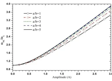
In both cases, the difference between the non-linear frequency and linear frequency increased by increasing the amplitude of vibration. This difference increased even more when aspect ratio in-creased (figure 2).

Figure 2 The effect of aspect ratio on the nonlinear to the linear frequency ratio

In table 2, the Variation of frequency ratios versus non-dimensional amplitude ratio for symmet-rical and non-symmetsymmet-rical square plate arrangements are shown. The symmetsymmet-rical arrangement plates have the same frequency ratios values.

Table 2 Frequency ratio of composite square plate with different arrangements using various methods

) 25 . 0 , 5 . 0 / , 40 /

(E1 E2= G12 E2= ν12=

[90°/0°/0°/90°] [0°/90°/90°/0°]

[0°/90°/0°/90°]

h W/

Ref [4] HAM

LIM Ref [4]

HAM LIM

Ref [4] HAM

LIM

1.0535 1.0509

1.0509 1.0535

1.0509 1.0509

1.0634 1.0575

1.0575 0.25

1.2038 1.1891

1.1892 1.2038

1.1891 1.1892

1.2388 1.212

1.2121 0.5

1.4172 1.3872

1.3874 1.4172

1.3872 1.3874

1.4832 1.4305

1.4308 0.75

1.6691 1.6227

1.6232 1.6691

1.6227 1.6232

1.7679 1.6881

1.6886 1

1.8819 1.8827

1.9694 1.9703

1.25

2.2355 2.1563

2.1574 2.2355

2.1563 2.1574

2.4000 2.2659

2.2671 1.5

2.4408 2.4422

2.5724 2.5739

1.75

2.8439 2.7325

2.7342 2.8439

2.7325 2.7342

3.0729 2.8857

2.8876 2

(12)

Table 3 Frequency ratio of composite rectangular plate with different arrangements using various methods ) 2 / , 25 . 0 , 5 . 0 / , 40 /

(E1 E2= G12 E2= ν12= a b=

[90°/0°/0°/90°] [0°/90°/90°/0°]

[0°/90°/0°/90°]

h W/ Ref [4] HAM LIM Ref [4] HAM LIM Ref [4] HAM LIM 1.0340 1.0322 1.0322 1.1327 1.1297 1.1297 1.0645 1.0522 1.0535 0.25 1.1331 1.1226 1.1226 1.4674 1.4458 1.4461 1.2427 1.2156 1.2261 0.5 1.2798 1.2576 1.2577 1.8946 1.8531 1.8538 1.4905 1.46 1.4797 0.75 1.4593 1.4239 1.4242 2.3652 2.304 2.3052 1.7787 1.7463 1.7704 1 1.6119 1.6124 2.7777 2.7795 2.0531 2.0782 1.25 1.8777 1.8148 1.8155 3.3634 3.2644 3.2666 2.4178 2.3703 2.3955 1.5 2.0283 2.0292 3.7591 3.7619 2.6935 2.7184 1.75 2.3396 2.2493 2.2505 4.3949 4.2591 4.2622 3.0976 3.0205 3.045 2

Table 4 Frequency ratio of composite rectangular plate with different arrangements using various methods

) 4 / , 25 . 0 , 5 . 0 / , 40 /

(E1 E2= G12 E2= ν12= a b=

[90°/0°/0°/90°] [0°/90°/90°/0°]

[0°/90°/0°/90°]

Tables 5 to 7 summarize comparison results for different modulus ratios.

Table 5: Frequency ratio of composite rectangular plate with different arrangements using various methods

) 25 . 0 , 5 . 0 / , 10 /

(E1 E2= G12 E2= ν12=

[90°/0°/0°/90°] [0°/90°/90°/0°]

[0°/90°/0°/90°]

(13)

Table 6 Frequency ratio of composite rectangular plate with different arrangements using various methods ) 2 / , 25 . 0 , 5 . 0 / , 10 /

(E1 E2= G12 E2= ν12= a b=

[90°/0°/0°/90°] [0°/90°/90°/0°]

[0°/90°/0°/90°]

Table 7 Frequency ratio of composite rectangular plate with different arrangements using various methods

) 4 / , 25 . 0 , 5 . 0 / , 10 /

(E1 E2= G12 E2= ν12= a b=

[90°/0°/0°/90°] [0°/90°/90°/0°]

[0°/90°/0°/90°]

It can be concluded from data given in tables above that frequency ratio increases with an in-crease in aspect ratio and modulus ratio and dein-creases when number of layers inin-creases. It should be noted that added number of layers will result in a raise of the frequency ratio.

6 CONCLUSION

(14)

References

[1] Chu HN, Herrmann G. Plate Influence of large amplitudes on free flexural vibrations of rectangular plates. ASME J Appl Mech 1956;23:532-540.

[2] Singha MK, Daripa R. Nonlinear vibration of symmetrically laminated composite skew plates by finite ele-ment method. International Journal of Non-Linear Mechanics 2007;42(9)1144-1152.

[3] Raju IS, Rao GV, Raju KK. Effect of longitudinal or inplane deformation and inertia on the large ampli-tude flexural vibrations of slender beams and thin plates. Journal of Sound and Vibration 1976;49(3):415-422.

[4] Singh S, Raju KK, Rao GV. Non-linear vibrations of simply supported rectangular cross-ply plates. Journal of Sound and Vibration 1990;142(2):213-226.

[5] Singha MK, Ganapathi M. Large amplitude free flexural vibrations of laminated composite skew plates. In-ternational Journal of Non-Linear Mechanics.2004;39(10):1709-1720.

[6] Malekzadeha P, Karami G. Differential quadrature nonlinear analysis of skew composite plates based on FSDT. Engineering Structures 2006;28(9)p1307-1318.

[7] Pirbodaghi T, Ahmadian MT, Fesanghary M. On the homotopy analysis method for nonlinear vibration of beams. Mechanics Research Communications 2009;36(2):143-148.

[8] Younesian D, Askari H, Saadatnia Z, KalamiYazdi M. Frequency analysis of strongly nonlinear generalized Duffing oscillators using He’s frequency amplitude formulation and He’s energy balance method. Comput Math Appl 2010;59:3222-3228.

[9] Yue YS, Lu FM. The max_min approach to a relativistic equation. Computers and Mathematics with Ap-plications 2009;58: 2131_2133.

[10] He JH. Homotopy perturbation method for solving boundary value problems. Phys Lett 2006;A 350:87-88. [11] He JH. Some asymptotic methods for strongly nonlinear equations. International Journal of Modern Physics

B 2006;20(10):1141-1199.

[12] Rafieipour H,Lotfavar A, Mansoori MH. New analytical approach to nonlinear behavior study of asymmet-rically LCBs on nonlinear elastic foundation under Steady axial and thermal loading. Latin American Jour-nal of Solids and Structures 2012;9(5):531-545.

[13] Reddy J. Mechanics of Laminated Composite Plates Theory and Analysis: CRC, Boca Raton, 1997. [14] Rao SS. Vibration of Continuous Systems: John Wiely & Sons, New Jersy, 2007.

(15)

Appendix

i

Ι

coefficients in the second approximation of deflection.

2 2 2 2 2 3

0 1 3 4 3 5 4 3 4 5 4 3 4

21 1 49 41 2 13 31 23

990904320A + -2 A + - + - + - A+ +

-16 32 512 48 3 4096 72 36

⎛⎛ ⎞ ⎛ ⎛ ⎞ ⎞ ⎛ ⎞ ⎞

Ι = ⎜_⎝⎜Π Π Π _⎠⎟ ⎜ Π _⎝⎜ Π Π Π_⎠⎟ Π ⎟ ⎜_⎝ Π Π Π⎟_⎠ Π ⎟

⎝ ⎠

(

)

(

)

(

)

(

)

(

)

4 3

1 5 3 1 2 4

2 2 2 2

3 4 5 3 5 4

2 2 3 3

4 5 3 4 5

=1981808640A -54190080 -1052835840 -1101004800 -7741440 1761607680 A

26512128 -595574784 101007360 -7741440 399114240 A

-457900032 -3740640 690880512 574560 A-14364

Ι + _Π _Π _Π _Π + _Π

+ _Π + _Π + _{Π Π} _Π + _Π +

Π Π Π + _Π + _Π Π45

(

)

2 2 2 2 2 3

2 1 3 4 3 4 5 3 4 4 5 3 4

1 51 7 3 2

110100480A -3 +2 A + - + -2 - +2 A+ +

-64 1024 16 512 3

⎛ ⎛ ⎛ ⎞ ⎞ ⎛ ⎞ ⎞

Ι = _⎜ Π Π Π _⎜ Π _⎜ Π Π Π_⎟ Π _⎟ _⎜ Π Π Π_⎟ Π _⎟

⎝ ⎠ ⎝ ⎠

⎝ ⎠

(

)

(

)

(

)

(

)

2

3 5 4 3

3 2

3 2 5 3

2 2

5 4

2 2 3 3 4

5 4 3 5 4 5

8547840 + 3870720 -45158400

7741440 +54190080 +61931520 A + A

+5806080 +41287680

+ -181440 -16629760 -544320 +13762560 A+15120

⎛ Π Π Π Π ⎞

Ι = Π Π Π ⎜ ⎟

⎜ _Π _Π ⎟

⎝ ⎠

Π Π Π Π Π Π

2 2 2 3

4 3 3 5 4 3 4 5 3 4

1 49 2 3 4

20643840A A - -6 + A+ - + +

10 16 45 320 45

⎛ ⎛ ⎞ ⎛ ⎞ ⎞

Ι = _⎜ Π Π _⎜ Π Π Π _⎟ _⎜ Π Π Π_⎟ Π _⎟

⎝ ⎠ ⎝ ⎠

⎝ ⎠

2 3

2 2 2 5 5

5 3 5 4 3 5 4 3

8 40 32

-483840A + - - -4 A+ - + +

3 9 27 24 8

⎛⎛ ⎛ ⎞ ⎞ ⎛ Π ⎞ Π ⎞

Ι = ⎜⎜Π ⎜_⎝ Π Π Π Π⎟_⎠ ⎟ ⎜ Π ⎟Π ⎟

⎝ ⎠ ⎝ ⎠

⎝ ⎠

2 2

6 3 3 5 5 4

51 3 4

147456A + A- +

16 8 9

⎛⎛ ⎞ ⎞

Ι = Π _⎜_⎜Π Π _⎟ Π Π _⎟

⎝ ⎠

(

)

2 2 2 4

7 26880 3A +10080 5 3 5+ 3 A-945 5

Ι = _Π _Π _{Π Π} _Π

2 8 3840 5A 3

Ι = Π Π

Ι9=189Π54

where

3 4 3

2 2

1 3 2 3 3

1 2 2

1 4 , 2 4 , 3 4 , 4 2 , 5 2

A A A

A

α

A

α

ω