Abstract
In the present work, a layerwise trigonometric shear deformation theory is used for the analysis of two layered (90/0) cross ply lami-nated simply supported and fixed beams subjected to sinusoidal load. The displacement field of the present theory consists of trigonometric sine function in terms of thickness coordinate to take into account the effect of transverse shear deformation. Theory satisfies the trans-verse shear stress free boundary conditions at top and bottom surfac-es of the beam. This model satisfisurfac-es the constitutive relationship between shear stress and shear strain in both the layers and the axial displacement compatibility at the interface. Virtual work principle is employed to obtain governing equations and boundary conditions. Closed form solution technique has the limitation of simply supported boundary condition. In the present work general solution technique is developed, which can be used for any type of boundary and loading conditions. The transverse shear stresses are obtained using constitu-tive relation as well from the use of equilibrium equations. The re-sults of displacements and stresses obtained by present theory are compared with the available results in the literature.
Key words
Shear deformation; cross-ply laminated beam; trigonometric shear deformation theory.
Flexural analysis of cross-ply laminated beams using layerwise
trigonometric shear deformation theory
1 INTRODUCTION
Structural elements made up of fiber reinforced composite material are being used in the aeronau-tical and aerospace industries as well as in the other fields of modern technology, primarily due to their high strength to weight ratio and stiffness to weight ratios and also due to their anisotropic material properties that can be achieved through variation of the fiber orientation and stacking sequence. The ratio of transverse shear modulus to elastic modulus is low for composites, hence shear deformation effects are more pronounced in the composite beams subjected to transverse loads. Analytical and numerical methods can be employed for the analysis of structural systems composed of laminated composite components.
The classical beam theory developed by Euler–Bernoulli (ETB) is used only for thin beams because this theory has neglected both transverse shear and normal strains. Timoshenko [1] has
Y. M. G h ug al an d S. B. Sh ind e*
Department of Applied Mechanics, Gov-ernment Engineering College,
Aurangabad - 431005, Maharashtra State, India
Received 26 Fev 2012 In revised form 12 Jun 2012
Nomenclature
b = Width of beam
D = Modified flexural rigidity coefficient as defined in Appendix
D1,D2,D3,D3 = Constants as defined in Appendix
D = Flexural rigidity
E(1), E(2) = Young’s moduli of layer 1and layer 2, respectively
h = Depth (i.e. thickness) of beam
L = Span of the beam
S = Aspect ratio (i.e. ratio of span to depth of beam)
x, y, z = Rectangular coordinates
α = Neutral axis coefficient as defined in Appendix
u = Non-dimensional axial displacement
w = Non-dimensional transverse displacement
σ
x = Non-dimensional axial stress
τ
zx
CR = Non-dimensional transverse shear stress obtained from the constitutive
rela-tionship
τ zx
EE = Non-dimensional transverse shear stress obtained from the equilibrium
equa-tions
Abbreviations
Superscripts
CR Constitutive relationships
EE Equilibrium equations
Acronyms
ETB Elementary theory of beam bending
FSDT First-order shear deformation theory
HSDT Higher order shear deformation theory
FEM Finite element method
LTSDT Layerwise trigonometric shear deformation theory,
HOSTB5 Higher order shear deformation theory
HST Higher order shear deformation theory
developed a thick beam theory to include the effect of the transverse shear deformation. This theory is widely known as first order shear deformation theory (FSDT). This theory assumes a constant shear strain across the thickness of the beam and requires a shear correction factor. However, this factor is problem dependent which is influenced by boundary conditions, loading conditions and stacking sequence of plies in the laminated beams.
In order to overcome the drawbacks of classical and Timoshenko beam theories, higher order or equivalent shear deformation theories have been developed. Research on analytical and numer-ical modeling of laminated composites has been very active in order to achieve accurate represen-tation of the actual behavior of this kind of structures. Ghugal and Shimpi [2], Reddy [3] and Kreja [4] provided comprehensive reviews of shear deformation theories for laminated beams and plates including merits and demerits of equivalent single layer and layerwise shear deformation theories.
A higher-order beam model formulated by Kant and Manjunatha [5] does not require any shear correction factor, where the model is based on a non-linear variation of longitudinal dis-placements through the beam thickness. Soldato [6] presented higher order model for cylindrical bending of cross-ply laminated plate with various boundary conditions subjected to single sinus-oidal transverse load. Zenkour [7] has developed higher order shear deformation beam theory. Analytical solution of theory is obtained using the Navier solution for simply supported boundary conditions.
Manjunatha and Kant [8], Maiti and Sinha [9], Vinayak et al. [10] used the equivalent single layer, displacement based, higher-order shear deformation theories (HSDT) in the analysis of symmetric and unsymmetric laminated beams and obtained the results using finite element meth-od. These theories are the special cases of Lo et al [11] higher-order theory.
Park and Lee [12] presented a new laminated plate theory in which the inplane displacements vary exponentially through plate thickness. The results based on this theory are obtained for symmetric / antisymmetric cross-ply, angle-ply and unsymmetric laminates under cylindrical bending. Khdeir and Reddy [13] used the state space concept in conjunction with the Jordan canonical form to solve the governing equations for the bending of cross-ply laminated composite beams. The classical, first-order, second-order and third-order theories have been used in the analysis.
Tahani [14] presented a displacement based layerwise beam theory and applied it to the lami-nated (0/90 and 0/90/0) beams subjected to a sinusoidal load. Liu and Li [15] compared different laminate theories based on displacement hypothesis emphasizing the importance of layerwise the-ories and also presented a series of quasi-layerwise thethe-ories. Li and Liu [16] presented results of single-layered, two-layered, three-layered cross-ply laminates for cylindrical bending The theory is layer dependent and the number of degrees of freedom involved is very
high and hence it is computationally complicated. Icardi [17] and Arya [18] presented zig-zag layerwise theories for the analysis of thick laminated beams.
for-
mulation and obtained results for un-symmetric cross-ply laminated beams using closed form ana-lytical solution. Shimpi and Ghugal [22] developed a simple layerwise trigonometric shear defor-mation theory which satisfies zero transverse shear stress condition at the top and bottom of the beam. The theory also satisfies the shear stress continuity condition at the interface between the layers. The theory includes a minimum number of displacement variables. A closed form analyti-cal solution is presented to obtain the results for beams with simply supported boundary condi-tions.
In the present paper a previously developed layerwise theory [22] is used and results are ob-tained for two layered cross ply laminated beams subjected to sinusoidal load with simply sup-ported and fixed-fixed boundary conditions. A general solution technique is developed which can be applied to beam with any type of loading and boundary conditions.
2 THEORETICAL FORM ULATION
The variationally correct forms of differential equations and boundary conditions, based on the assumed displacement field, are obtained using the principle of virtual work. The beam under consideration consists of two layers: layer 1 and layer 2.
Layer 1 (900 layer) occupies the region:
0 ≤ x ≤ L; –b/2 ≤ y ≤ b/2; –h/2 ≤ z ≤ 0 (1)
Layer 2 (00 layer) occupies the region:
0 ≤ x ≤ L; –b/2 ≤ y ≤ b/2; 0 ≤ z ≤ h/2 (2)
where x, y, z are Cartesian coordinates, L is the length, b is the width and h is the total depth of beam. The beam can have meaningful boundary conditions and loading conditions.
The beam subjected to transverse load and geometry of the cross-section is shown in Fig.1.
Figure 1 Composite beam with a transverse distributed load and geometry of the cross- section,
y
x, u
z
b
h
L
z, w
q( x )
2.1 Displacement field
The displacement field of the present beam theory is of the form [22] as given below:
u(1)(x,z)=−(z−αh)dw
dx +h C1+C2sin
π 2
z /h−α 0.5+α ⎛ ⎝ ⎜⎜ ⎜ ⎞ ⎠ ⎟⎟ ⎟⎟ ⎡ ⎣ ⎢ ⎢ ⎤ ⎦ ⎥
⎥φ(x) (3)
u(2)(x,z)=−(z−αh)dw
dx +h C3+sin
π 2
z /h−α 0.5−α ⎛ ⎝ ⎜⎜ ⎜ ⎞ ⎠ ⎟⎟ ⎟⎟ ⎡ ⎣ ⎢ ⎢ ⎤ ⎦ ⎥
⎥φ(x) (4)
w (x,z)=w(x) (5)
Here u(1) and u(2) are the axial displacement components in the x direction, superscripts 1 and 2 refer to layer 1 and layer 2; w(x) is the transverse displacement in the z direction and C1, C2, C3 and α are the constants as given in Appendix. The function φ(x)is a rotation function or the warping function of the cross-section of the beam.
2.2 Strains
Normal and transverse shear strains for layer 1 and 2 are as follows:
εx
(1)=du(1) dx =−(
z−αh)d 2w
dx2
+h C
1+C2sin π 2
z/h−α 0.5+α ⎛ ⎝ ⎜⎜ ⎜ ⎞ ⎠ ⎟⎟ ⎟⎟ ⎡ ⎣ ⎢ ⎢ ⎤ ⎦ ⎥ ⎥ dφ
dx (6)
εx
(2) =du(2) dx =−(
z −αh)d 2w
dx2
+h C 3+sin
π
2
z /h−α 0.5−α ⎛ ⎝ ⎜⎜ ⎜ ⎞ ⎠ ⎟⎟ ⎟⎟ ⎡ ⎣ ⎢ ⎢ ⎤ ⎦ ⎥ ⎥ dφ
dx (7)
γzx(1) =du (1) dz + dw dx = πC 2
1+2αcos π 2
z /h−α 0.5+α ⎛ ⎝ ⎜⎜ ⎜ ⎞ ⎠ ⎟⎟
⎟⎟φ (8)
γzx(2)=du (2)
dz +
dw
dx = π 1−2αcos
π 2
z/h−α 0.5−α ⎛ ⎝ ⎜⎜ ⎜ ⎞ ⎠ ⎟⎟
⎟⎟φ (9)
2.3 Stresses
One dimensional constitutive law are used to obtain the normal bending and transverse shear stresses for layer 1 and layer 2 as given below:
σx(1) =E(1)ε x
(1)=E(1)(z−αh)d2w dx2
+E(1)h C
1+C2sin π 2
z /h−α 0.5+α
⎛ ⎝ ⎜⎜ ⎜ ⎞ ⎠ ⎟⎟ ⎟⎟ ⎡ ⎣ ⎢ ⎢ ⎤ ⎦ ⎥ ⎥ dφ
σx
(2)=E(2)ε x
(2)=−E(2)(z−αh)d2w dx2
+E(2)h C 3+sin
π 2
z/h−α 0.5−α
⎛ ⎝ ⎜⎜ ⎜
⎞ ⎠ ⎟⎟ ⎟⎟ ⎡
⎣ ⎢ ⎢
⎤
⎦ ⎥ ⎥
dφ
dx (11)
τzx
(1) =G(1)γ zx
(1) =G(1) πC2
1+2αcos π 2
z /h−α
0.5+α ⎛
⎝ ⎜⎜ ⎜
⎞ ⎠ ⎟⎟
⎟⎟φ (12)
τzx
(2)
=G(2)γ zx
(2)
=G(2) π 1−2αcos
π 2
z /h−α 0.5−α ⎛
⎝ ⎜⎜ ⎜
⎞ ⎠ ⎟⎟
⎟⎟φ (13)
2.4 Governing Equations and Boundary Conditions
Using the expressions (6) to (13) for strains and stresses and principle of virtual work, variation-ally consistent differential equations and boundary conditions for the beam under consideration are obtained. The principle of virtual work applied to beam is as follows:
b
(
σx(1)δεx(1)+τzx(1)δγzx(1))
z=−h/2z=0
∫
x=0 x=L
∫
dxdz+b(
σx(2)δεx(2)+τzx(2)δγzx(2))
z=0z=h/2
∫
x=0 x=L
∫
dxdz− qδw dxx=0 x=L
∫
= 0 (14)where the symbol δ denotes the variational operator. Integrating the Eq. (14) by parts and
col-lecting the coefficients of the primary variables (i.e. w andφ), we obtain the governing equations and the associated boundary conditions. The governing equations are as follows:
d4w
dx4 −D1d
3
φ dx3
− q D =
0 (15)
dw3
dx3 −D
2 d2φ dx2
+D
3φ=0 (16)
The associated boundary conditions are of the following form:
d3w
dx3 −D
1 d2φ dx2 =
0 or w is prescribed (17)
d2w dx2
−D 1
dφ dx =
0 or dw
dx is prescribed (18)
d2w
dx2 −D
2 dφ dx =
0 or f is prescribed (19)
Thus, the static behavior of beam is given by the solution of these variationally consistent governing differential equations and simultaneously satisfaction of the associated boundary condi-tions.
2.5 The general solution for static flexure of beams
Using governing equations (15) and (16); general solution for w (x) and φ(x)can be obtained. By integrating and rearranging the equation (15), one can get the following equation:
d3
w
dx3 −D1
d2
φ dx2 =
Q x
( )
D (20)
where Q(x) =
∫
q dx+K1 is the generalized shear force resulting from the support and loading conditions for the beam under consideration. Using Eqs. (16) and (20), a single differential equa-tion in terms of φcan be obtained as follows:d2φ
dx2−λ
2φ =Q x
( )
ηD (21)
where the constants η and λ used in Eq.(21) are given in Appendix. The general solution of above Eq. (21) is given by:
φ(x)=K2coshλx + K3 sinhλx − Q(x)
ηD (22)
The general solution for transverse displacement (w) can be obtained by substituting the ex-pression for φ in Eq. (16) and integrating thrice with respect to x. The solution is
Dw x
( )
= q dx dx dx dx+K1x 36
∫
+K4x2
2
∫
∫
∫
+DD1D3
K2coshλx +K
3sinhλx ⎡
⎣ ⎤⎦+K5x+K6 (23)
where K1,K2,K3,K4,K5 and K6are the constants of integration and can be obtained using boundary conditions of the beam under consideration.
2.6 Axial stress and Transverse shear stresses
Final solutions for φ
( )
x and w (x) can be obtained using Eqs. (22) and (23) depending upon theloading and boundary conditions of the beams. Substituting the final solution for w (x) and φ
( )
x in the displacement field, the final displacement can be obtained. Finally, the axial stress σ
and (11). The transverse shear stress τ
xz can be obtained either by using the constitutive relation [Eqs. (12) and (13)] or by integrating equilibrium equation with respect to the thickness coordi-nate. Two-dimensional elasticity equilibrium equations by ignoring body forces can be used to obtain transverse shear stress. The equation is:
∂σ xx ∂x
+∂τxz ∂z
=0 (24)
Integrating Eq. (24), with respect to the thickness coordinate z and imposing the following boundary condition at top surface of the beam
τxz(1) ⎡
⎣⎢ ⎤⎦⎥z=−h/2 =0 (25)
Expression for τ
xz
(1) can be obtained. To maintain the continuity at interface, another
bounda-ry condition is applied, i.e.
τ
xz (1)
= τ
xz
(2) at z =0 (26)
From this condition expression for τ
xz
(2) is obtained for layer 2 which satisfies the requirement of zero transverse shear stress condition on the bottom surface of the beam.
3. ILLUSTRATIVE EXAM PLES
To verify the accuracy of the theory two examples of two layered un-symmetric cross ply lami-nated beams with simply supported and fixed boundary conditions and subjected to sinusoidal loading are analysed. From the analysis the effect of shear deformation and stress concentration on the displacements and stresses is investigated. The material of the beam layers is graph-ite/epoxy uni-directional composite. The following has been assumed:
E 2 ( )
E( )1
=25, G 1 ( )
E( )1
=0.20, G 2 ( )
E( )2
=0.02
Superscripts (1) and (2) refer to layer-1 and layer-2 respectively.
3.1 Example1: Simply supported beam with sinusoidal load q =q0sin
(
πx/L)
Dd
3w
dx3 = Dd
2 φ dx2 =
dw
dx =φ=
0 at x = L/2 (27)
Dd 2w
dx2 = Ddφ
dx =
w=0 at x = 0, L
(28)
The boundary condition, φ= 0 at x = L/2 is used from the condition of symmetry of
defor-mation, in which the middle cross-section of the beam must remain plane without warping (Gere and Timoshenko [23]). From the general solution of beam, expression for φ and ware obtained as follows:
φ(x)= q0L πDD3
cos
(
πx /L)
Ω (29)
w =q0L
4
π4D
χ Ωsin πx L ⎛ ⎝ ⎜⎜ ⎜ ⎞ ⎠ ⎟⎟ ⎟⎟ (30)
where, Ω= 1+ π
λL ⎛ ⎝ ⎜⎜ ⎜ ⎞ ⎠ ⎟⎟ ⎟⎟ 2 ⎡ ⎣ ⎢ ⎢ ⎢ ⎤ ⎦ ⎥ ⎥
⎥ and χ
= 1+π
2 L2 D2 D3 ⎡ ⎣ ⎢ ⎢ ⎤ ⎦ ⎥ ⎥
The expressions for displacements and stresses of the beam are obtained using this solution, which are as follows:
The axial displacement for Layer 1 is expressed as:
u( ) =1 q0
D −
(
z−αh)
L3π3 χ Ω+
Lh
πD3Ω C1+C2sin π 2
z /h−α
(
)
0.5+α ⎛ ⎝ ⎜⎜ ⎜⎜ ⎞ ⎠ ⎟⎟ ⎟⎟⎟ ⎡ ⎣ ⎢ ⎢ ⎢ ⎤ ⎦ ⎥ ⎥ ⎥ ⎧ ⎨ ⎪⎪ ⎩ ⎪⎪ ⎫ ⎬ ⎪⎪ ⎭ ⎪⎪cos πx L ⎛ ⎝ ⎜⎜ ⎜ ⎞ ⎠ ⎟⎟ ⎟⎟ (31)
The axial displacement for Layer 2 is expressed as:
u( ) =2 q0
D −
(
z−αh)
L3π3 χ Ω+
Lh
πD3Ω C3+sin π 2
z /h−α
(
)
0.5−α ⎛ ⎝ ⎜⎜ ⎜⎜ ⎞ ⎠ ⎟⎟ ⎟⎟⎟ ⎡ ⎣ ⎢ ⎢ ⎢ ⎤ ⎦ ⎥ ⎥ ⎥ ⎧ ⎨ ⎪⎪ ⎩ ⎪⎪ ⎫ ⎬ ⎪⎪ ⎭ ⎪⎪cos πx L ⎛ ⎝ ⎜⎜ ⎜ ⎞ ⎠ ⎟⎟ ⎟⎟ (32)
The axial stress for Layer 1 is expressed as:
σx( ) =1 E
1
( )
(
z−αh)
q0L 2
π2D
χ Ωsin πx L ⎛ ⎝ ⎜⎜ ⎜ ⎞ ⎠ ⎟⎟ ⎟⎟ −
E( )1q0h
DD3Ω C1+C2sin π
2
z /h−α
(
)
0.5+α ⎛ ⎝ ⎜⎜ ⎜⎜ ⎞ ⎠ ⎟⎟ ⎟⎟⎟ ⎡ ⎣ ⎢ ⎢ ⎢ ⎤ ⎦ ⎥ ⎥ ⎥ sin πx L ⎛ ⎝ ⎜⎜ ⎜ ⎞ ⎠ ⎟⎟ ⎟⎟ (33)
σx( ) =2 E 2
( )
(
z−αh)
q0L2
π2D
χ Ωsin πx L ⎛ ⎝ ⎜⎜ ⎜ ⎞ ⎠ ⎟⎟ ⎟⎟ −
E( )2q0h
DD3Ω C3+sin π 2
z /h−α
(
)
0.5−α ⎛ ⎝ ⎜⎜ ⎜⎜ ⎞ ⎠ ⎟⎟ ⎟⎟⎟ ⎡ ⎣ ⎢ ⎢ ⎢ ⎤ ⎦ ⎥ ⎥ ⎥sin πx L ⎛ ⎝ ⎜⎜ ⎜ ⎞ ⎠ ⎟⎟ ⎟⎟ (34)
The transverse shear stress using constitutive relationship for Layer 1 is expressed as:
τ zx
1
( ) = q0L DD3Ω
G( )1C2 1+2α
(
)
cosπ
2
z /h−α
0.5+α ⎛ ⎝ ⎜⎜ ⎜ ⎞ ⎠ ⎟⎟ ⎟⎟cos πx L (35)
The transverse shear stress using constitutive relationship for Layer 1 is expressed as:
τ
zx 2
( ) = q0L DD3Ω
G( )2 1−2α
(
)
cosπ
2
z/h−α
0.5−α ⎛ ⎝ ⎜⎜ ⎜ ⎞ ⎠ ⎟⎟ ⎟⎟cos πx L (36)
The transverse shear stress using equilibrium equation for Layer 1 is expressed as:
τzx( ) =1 q0 D
E( )1χL Ωπ
z2
2 −αhz+ h2
8 +
αh2 2 ⎛ ⎝ ⎜⎜ ⎜⎜ ⎞ ⎠ ⎟⎟ ⎟⎟⎟cos πLx
⎛ ⎝ ⎜⎜ ⎜ ⎞ ⎠ ⎟⎟ ⎟⎟ +E 1 ( )hπ
ΩLD3 zC1+C2
h
(
1+2α)
π cos
π
2
z/h−α
(
)
0.5+α
⎛ ⎝ ⎜⎜ ⎜⎜ ⎞ ⎠ ⎟⎟ ⎟⎟⎟+hC1
2 ⎡ ⎣ ⎢ ⎢ ⎢ ⎤ ⎦ ⎥ ⎥ ⎥cos πx L ⎛ ⎝ ⎜⎜ ⎜ ⎞ ⎠ ⎟⎟ ⎟⎟ ⎧ ⎨ ⎪⎪ ⎪⎪ ⎪⎪ ⎩ ⎪⎪ ⎪⎪ ⎪⎪ ⎫ ⎬ ⎪⎪ ⎪⎪ ⎪⎪ ⎭ ⎪⎪ ⎪⎪ ⎪⎪ (37)
The transverse shear stress using equilibrium equation for Layer 2 is expressed as:
τzx( )2 =q0 D
+E 1 ( )L
π χ
Ω h2
8 +
αh2 2 ⎛ ⎝ ⎜⎜ ⎜⎜ ⎞ ⎠ ⎟⎟ ⎟⎟⎟cos πLx
⎛ ⎝ ⎜⎜ ⎜ ⎞ ⎠ ⎟⎟ ⎟⎟ −E
2 ( )L
π χ
Ω z2
2 −αhz
⎛ ⎝ ⎜⎜ ⎜⎜ ⎞ ⎠ ⎟⎟ ⎟⎟⎟cos πLx
⎛ ⎝ ⎜⎜ ⎜ ⎞ ⎠ ⎟⎟ ⎟⎟ −E 1 ( )hπ
LD3Ω −
hC1 2 ⎛ ⎝ ⎜⎜ ⎜⎜ ⎞ ⎠ ⎟⎟ ⎟⎟+C2
h
(
1+2α)
π cos
π 2
−α 0.5+α
⎛ ⎝ ⎜⎜ ⎜ ⎞ ⎠ ⎟⎟ ⎟⎟ ⎡ ⎣ ⎢ ⎢ ⎢ ⎤ ⎦ ⎥ ⎥ ⎥
cos πx L ⎛ ⎝ ⎜⎜ ⎜ ⎞ ⎠ ⎟⎟ ⎟⎟ +E 2 ( )hπ
LD3Ω zC3+
h
(
1−2α)
π cos
π 2
z/h−α
(
)
0.5−α
⎛ ⎝ ⎜⎜ ⎜⎜ ⎞ ⎠ ⎟⎟
⎟⎟⎟+h
(
1−π2α)
cos π 2−α 0.5−α
⎛ ⎝ ⎜⎜ ⎜ ⎞ ⎠ ⎟⎟ ⎟⎟ ⎡ ⎣ ⎢ ⎢ ⎢ ⎤ ⎦ ⎥ ⎥ ⎥
cos πx L ⎛ ⎝ ⎜⎜ ⎜ ⎞ ⎠ ⎟⎟ ⎟⎟ ⎧ ⎨ ⎪⎪ ⎪⎪ ⎪⎪ ⎪⎪ ⎪⎪ ⎩ ⎪⎪ ⎪⎪ ⎪⎪ ⎪⎪ ⎪⎪ ⎫ ⎬ ⎪⎪ ⎪⎪ ⎪⎪ ⎪⎪ ⎪⎪ ⎭ ⎪⎪ ⎪⎪ ⎪⎪ ⎪⎪ ⎪⎪ (38)
Table 1 Non-dimensional maximum transverse displacement ( w) at(x=0.5L,z=0), axial displacement ( u) at
(x =0,z= ±h/ 2), axial stress (σ
x) at (
x =0.5L,z= ±h/ 2), and transverse shear stresses (τ xz) at (
x = 0.0, z =ah)for
simply supported beam subjected to sinusoidal load q=q0sin
(
πx/L)
with aspect ratio, S = 4 (Example: 1)Source
(Model) w
u σx τ
xz CR
τ xz EE
‐ h/2 h/2 ‐ h/2 h/2
Present (LTSDT) 4.7437 5.0353 ‐ 1.5574 3.9547 ‐ 30.5650 2.9895 2.6784
Bernoulli- Euler (ETB) 2.6281 3.8574 ‐ 1.4216 3.0386 ‐ 27.9540 -- 2.9453
Timoshenko [1] (FSDT) 4.7967 3.8574 ‐ 1.4216 3.0386 ‐ 27.9540 1.8189 2.9453
Ghugal and Shimpi [22], (LTSDT-II) 4.7437 5.0353 --- 3.9547 ‐ 30.5650 2.9895 2.6784 Kant and Manjunatha [5] (FSDT/FEM) 4.2828 4.8611 --- 3.7490 ‐ 27.0500 1.9270 2.8240
Lu and Liu [20] (HSDT) 4.7773 4.7143 --- 3.5714 ‐ 30.0000 2.7925 --
Maiti and Sinha [9] (HST/FEM) 3.5346 --- --- 2.3599 ‐ 25.7834 --- 2.4252
Maiti and Sinha [9] (FSDT/ FEM) 4.7898 --- --- 3.1514 ‐ 29.1144 2.8467 ---
Vinayak et al. [10] (HSDT/ FEM) 4.5619 --- --- 4.0000 ‐ 27.0000 --- 2.7500
Catapano et al [21] for N = 3
4.5733 4.4228 --- 3.7491 ‐ 28.757 2.1854
(0.25L) ---
Ghugal [24] (Exact Solution) 4.6616 4.5685 ‐ 1.5288 3.8381 ‐ 30.0190 2.7212 ---
Figure in parenthesis indicate the distance x from left end of the beam.
Table 2 Nondimensional maximum transverse displacement
( )
w at (x=0.5L,z=0)axial displacement ( u) at(x =0,z= ±h/ 2), axial stress (σ
x) at(
x =0.5L,z= ±h/ 2), and transverse shear stresses (τ
xz) at (x = 0.0, z = h a ) for
simply supported beam subjected to sinusoidal loadq =q0sin
(
πx/L)
with aspect ratio, S = 10 (Example: 1)Source
(Model) w
u
x s
CR xz
t EE
xz
t
‐ h/2 h/2 ‐ h/2 h/2
Present (TSDT) 2.9744 63.305 ‐ 22.563 19.888 ‐ 177.14 7.6948 7.2609
Bernoulli- Euler (ETB) 2.6281 60.354 ‐ 22.213 18.935 ‐ 174.71 -- 7.3643
Timoshenko [1] (FSDT) 2.9730 60.354 ‐ 22.213 18.935 ‐ 174.71 4.5473 7.3643
Ghugal and Shimpi [22] (LTSDT-II) 2.9744 63.305 -- 19.888 ‐ 174.71 7.6948 7.2638
Manjunatha and Kant
[8] (HOSTB5/ FEM) 2.8986 -- -- 19.710 ‐ 173.00 4.9130 7.2820
Lu and Liu [20]
(HSDT) 3.0000 61.666 -- 20.000 ‐ 175.00 7.3000 --
Catapano et al [ 21 ]
for N = 3 2.9332 61.637 --- 19.693
‐ 175.31 5.5649 (0.25L) Ghugal[24]
(Exact Solution) 2.9613 62.326 ‐ 22.476 19.830 ‐ 176.53 7.2678 ---
Figure 2 Variation of maximum transverse displacement (w) of simply supported beam at (x = L/2, S) when subjected to sinusoidal load
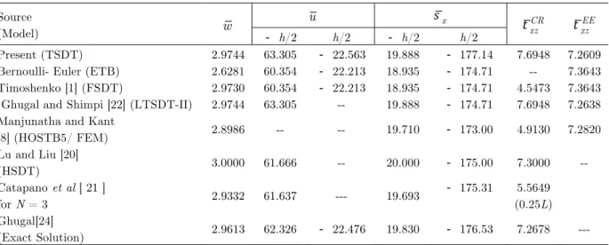
Figure 3 Variation of axial displacement ( u) through the thickness of simply supported beam at (x =0,z) when subjected to sinusoidal load for aspect ratio 4
0 10 20 30 40 50
S 2
4 6 8 10 12
w
ETB
FSDT
TSDT
-2 -1 0 1 2 3 4 5 6
u -0.50
-0.25
0.00
0.25
0.50 z/h
ETB
FSDT
Figure 4 Variation of axial displacement ( u) through the thickness of simply supported beam at (x =0,z) when subjected to sinusoidal load for aspect ratio 10
Figure 5 Variation of axial stress (σ
x) through the thickness of simply supported beam at (x =L/ 2,z) when subjected to sinus-oidal load for aspect ratio 4
-30 -15 0 15 30 45 60 75
u
-0.50
-0.25
0.00
0.25
0.50
z/h
ETB
FSDT
TSDT
-40 -30 -20 -10 0 10 20 30
σx
-0.50
-0.25
0.00
0.25
0.50
z/h
Figure 6 Variation of Axial stress (σ
x) through the thickness of simply supported beam at (
x =L/ 2,z) when subjected to
sinus-oidal load for aspect ratio 10
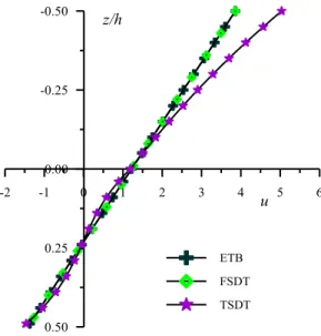
Figure 7 Variation of transverse shear stress (τ
zx) through the thickness of simply supported beam at (x =0.0 ,L z) when sub-jected to sinusoidal load and obtained using constitutive relations for aspect ratio 4
-225 -150 -75 0 75 150
σx
-0.50
-0.25
0.00
0.25
0.50 z/h
ETB
FSDT
TSDT
0 1 2 3
τzx -0.50
-0.25
0.00
0.25
0.50
z/h FSDT
Figure 8 Variation of transverse shear stress (τ
zx) through the thickness of simply supported beam at(
x =0.0L,z) when
sub-jected to sinusoidal load and obtained using constitutive relations for aspect ratio 10
Figure 9 Variation of transverse shear stress (τ
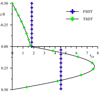
zx) through the thickness of simply supported beam at (x =0,z) when subjected to sinusoidal load and obtained using equilibrium equations for aspect ratio 4
0 1 2 3 4 5 6 7 8
τzx
-0.50
-0.25
0.00
0.25
0.50
z/h FSDT
TSDT
-1 0 1 2 τzx 3
-0.50
-0.25
0.00
0.25
0.50
z/h ETB
FSDT
Figure 10 Variation of transverse shear stress (τ
zx) through the thickness of simply supported beam at (x =0,z) when subject-ed to sinusoidal load and obtainsubject-ed using equilibrium equations for aspect ratio 10
3.2 Example 2: Fixed beam with sinusoidal load q =q0sin
(
πx /L)
A fixed-fixed beam with rectangular cross-section (b×h) is considered. The beam is subjected to sinusoidal load over the span L at surface z = – h/2. The origin of the beam is at left end sup-port, i.e. at x = 0. The boundary conditions associated with fixed beam are as follows:
Ddw dx =
Dw =0 at x =0 (39)
Dd 3
w
dx3 = Dd
2
φ
dx2= Ddw
dx=
0 atx=L
2 (40)
φ=0 atx=0,L
2 (41)
Thus, the general solution for φ and w are obtained as follows:
φ(x)=ξ
(
sinhλx−coshλx+cosπx/L)
when 0≤x ≤L/ 2 (42)where ξ= q0L πDD3Ω
-2 0 2 4 6 8
τzx
-0.50
-0.25
0.00
0.25
0.50
z/h
ETB
FSDT
w(x)=q0L4 π4D
χ
Ω sin(πx/L)−
(
πx/L)
+ πx2/L2
(
)
⎡
⎣⎢ ⎤⎦⎥+
q0L2 πD
D1 D3Ω
coshλx−sinhλx−1
λL + x L− x2 L2 ⎡ ⎣ ⎢ ⎢⎢ ⎤ ⎦ ⎥ ⎥⎥ (43)
when 0≤x≤L/ 2 where Ω= 1+ π 2
λ2L2 ⎛ ⎝ ⎜⎜ ⎜⎜ ⎞ ⎠ ⎟⎟
⎟⎟⎟,χ= 1+D2
D3 π2 L2 ⎛ ⎝ ⎜⎜ ⎜⎜ ⎞ ⎠ ⎟⎟ ⎟⎟⎟,
The expressions for displacement and stresses of the beam are obtained using this solution, are as follows:
The axial displacement for Layer 1 is expressed as:
u( )1 =q0 D
−
(
z−αh)
L3
π3 χ
Ω⎡⎣cos
(
πx/L)
−1+2(x/L)⎤⎦−
(
z−αh)
LπΩ
D1
D3 sinhλx−coshλx+1−2
(
x/L)
⎡
⎣ ⎤⎦
+ Lh
πD3Ω C1+C2sin
π
2
z/h−α
0.5+α
⎛ ⎝ ⎜⎜ ⎜ ⎞ ⎠ ⎟⎟ ⎟⎟ ⎡ ⎣ ⎢ ⎢ ⎤ ⎦ ⎥ ⎥f1(x)
⎧ ⎨ ⎪⎪ ⎪⎪ ⎪⎪ ⎪⎪ ⎪ ⎩ ⎪⎪ ⎪⎪ ⎪⎪ ⎪⎪ ⎪ ⎫ ⎬ ⎪⎪ ⎪⎪ ⎪⎪ ⎪⎪ ⎪ ⎭ ⎪⎪ ⎪⎪ ⎪⎪ ⎪⎪ ⎪ (44)
The axial displacement for Layer 2 is expressed as:
u( )2 =q0 D
−
(
z−αh)
L3
π3 χ
Ω⎡⎣cos
(
πx/L)
−1+2(x/L)⎤⎦−
(
z−αh)
LπΩ
D1
D3⎡⎣sinhλx−coshλx+1−2
(
x/L)
⎤⎦+ Lh
πD3Ω C3+sin
π
2
z/h−α
0.5−α
⎛ ⎝ ⎜⎜ ⎜ ⎞ ⎠ ⎟⎟ ⎟⎟ ⎡ ⎣ ⎢ ⎢ ⎤ ⎦ ⎥ ⎥f1(x)
⎧ ⎨ ⎪⎪ ⎪⎪ ⎪⎪ ⎪⎪ ⎪ ⎩ ⎪⎪ ⎪⎪ ⎪⎪ ⎪⎪ ⎪ ⎫ ⎬ ⎪⎪ ⎪⎪ ⎪⎪ ⎪⎪ ⎪ ⎭ ⎪⎪ ⎪⎪ ⎪⎪ ⎪⎪ ⎪ (45)
where f1(x)=sinhλx−coshλx+cos
(
πx/L)
The axial stress for Layer 1 is expressed as:
σx( )1 =q0 D
−E
(1)
(
z−αh)
L3π3
χ Ω
π
Lsin
(
πx/L)
+(2 /L) ⎡ ⎣ ⎢ ⎢ ⎤ ⎦ ⎥ ⎥ −E 1( )
(
z−αh)
LπΩ
D1
D3
(
λcoshλx−λsinhλx−2 /L)
+E 1 ( )λLh
πD3Ω C1+C2sin π
2
z/h−α
where f2(x)=coshλx−sinhλx− π
λLsin πx/L
(
)
The axial stress for Layer 2 is expressed as:
σx( )2 =q0 D
−E
(2)
(
z−αh)
L3π3
χ Ω
π
Lsin
(
πx/L)
+(2 /L) ⎡ ⎣ ⎢ ⎢ ⎤ ⎦ ⎥ ⎥ −E 2 ( ) z−αh
(
)
λLπΩ
D1
D3 coshλx−sinhλx− 2 λL ⎛ ⎝ ⎜⎜ ⎜ ⎞ ⎠ ⎟⎟ ⎟⎟ +E 2 ( ) λLh
πD3Ω C3+sin π
2
z/h−α
0.5−α ⎛ ⎝ ⎜⎜ ⎜ ⎞ ⎠ ⎟⎟ ⎟⎟ ⎡ ⎣ ⎢ ⎢ ⎤ ⎦ ⎥ ⎥f2(x) ⎧ ⎨ ⎪⎪ ⎪⎪ ⎪⎪ ⎪⎪ ⎪⎪ ⎩ ⎪⎪ ⎪⎪ ⎪⎪ ⎪⎪ ⎪⎪ ⎫ ⎬ ⎪⎪ ⎪⎪ ⎪⎪ ⎪⎪ ⎪⎪ ⎭ ⎪⎪ ⎪⎪ ⎪⎪ ⎪⎪ ⎪⎪ (47)
The transverse shear stress using constitutive relationship for Layer 1 is expressed as:
τzx( )1 =G 1 ( )ξ πC
2
1+2α
(
)
cosπ 2
z/h−α 0.5+α ⎛ ⎝ ⎜⎜ ⎜ ⎞ ⎠ ⎟⎟
⎟⎟f1(x) (48)
τzx( )2 = G 2
( )ξ π
1−2α
(
)
cosπ 2
z/h−α 0.5−α ⎛ ⎝ ⎜⎜ ⎜ ⎞ ⎠ ⎟⎟
⎟⎟f1(x) (49)
The transverse shear stress using equilibrium equations for Layer 1 is expressed as:
τzx( )1 =q0
D −E (1)L π χ Ω z2
2 −αhz− h2
8 −
αh2 2 ⎛ ⎝ ⎜⎜ ⎜⎜ ⎞ ⎠ ⎟⎟
⎟⎟⎟cos
(
πx/L)
+E
(1)λ2L2
πLΩ D1 D3
z2
2 −αhz− h2
8 −
αh2 2 ⎛ ⎝ ⎜⎜ ⎜⎜ ⎞ ⎠ ⎟⎟
⎟⎟⎟⎡⎣sinhλx−coshλx⎤⎦
−E
1
( )λ2L2h
πΩ
D1 D3 zC1−
h
(
1+2α)
π cos
π 2
z/h−α
0.5+α
⎛ ⎝ ⎜⎜ ⎜ ⎞ ⎠ ⎟⎟ ⎟⎟+ hC1 2 ⎛ ⎝ ⎜⎜ ⎜⎜ ⎞ ⎠ ⎟⎟ ⎟⎟⎟
sinhλx−coshλx− π
2
λ2L2cos
πx L ⎡ ⎣ ⎢ ⎢ ⎢ ⎤ ⎦ ⎥ ⎥ ⎥ ⎧ ⎨ ⎪⎪ ⎪⎪ ⎪⎪ ⎪⎪ ⎪⎪ ⎪⎪ ⎪⎪ ⎩ ⎪⎪ ⎪⎪ ⎪⎪ ⎪⎪ ⎪⎪ ⎪⎪ ⎪⎪ ⎫ ⎬ ⎪⎪ ⎪⎪ ⎪⎪ ⎪⎪ ⎪⎪ ⎪⎪ ⎪⎪ ⎭ ⎪⎪ ⎪⎪ ⎪⎪ ⎪⎪ ⎪⎪ ⎪⎪ ⎪⎪ (50)
τzx( ) =2 q0 D −E (2)L π χ Ω z2
2 −αhz ⎛ ⎝ ⎜⎜ ⎜⎜ ⎞ ⎠ ⎟⎟
⎟⎟⎟cosπLx+ E( )1L
π χ
Ω
h2
8 +
αh2
2 ⎛ ⎝ ⎜⎜ ⎜⎜ ⎞ ⎠ ⎟⎟ ⎟⎟⎟cosπLx
+E
(2)λ2L2
πLΩ
D1
D3 z2
2 −αhz ⎛ ⎝ ⎜⎜ ⎜⎜ ⎞ ⎠ ⎟⎟
⎟⎟⎟⎡⎣sinhλx−coshλx⎤⎦
−E
1
( )λ2L2
πLΩ
D1
D3 h2
8 +
αh2
2 ⎛ ⎝ ⎜⎜ ⎜⎜ ⎞ ⎠ ⎟⎟
⎟⎟⎟⎡⎣sinhλx−coshλx⎤⎦
−E
2
( )λ2L2h
πD3ΩL zC3−
h
(
1−2α)
π cos
π
2
z/h−α
0.5−α
⎛ ⎝ ⎜⎜ ⎜ ⎞ ⎠ ⎟⎟ ⎟⎟+
h
(
1−2α)
π cos
π
2 −α
0.5−α
⎛ ⎝ ⎜⎜ ⎜ ⎞ ⎠ ⎟⎟ ⎟⎟ ⎡ ⎣ ⎢ ⎢ ⎢ ⎤ ⎦ ⎥ ⎥ ⎥
sinhλx−coshλx− π
2
λ2L2cos πx L ⎡ ⎣ ⎢ ⎢ ⎢ ⎤ ⎦ ⎥ ⎥ ⎥ −E 1
( )λ2L2h
πD3ΩL −
h
(
1+2α)
π cos
π
2 −α
0.5+α
⎛ ⎝ ⎜⎜ ⎜ ⎞ ⎠ ⎟⎟ ⎟⎟+ hC1 2 ⎡ ⎣ ⎢ ⎢ ⎢ ⎤ ⎦ ⎥ ⎥ ⎥
sinhλx−coshλx− π
2
λ2L2cos πx L ⎡ ⎣ ⎢ ⎢ ⎢ ⎤ ⎦ ⎥ ⎥ ⎥ ⎧ ⎨ ⎪ ⎪ ⎪ ⎪ ⎪ ⎪ ⎪ ⎪ ⎪ ⎪ ⎪ ⎪ ⎪ ⎪ ⎪ ⎪ ⎪ ⎪ ⎪ ⎪ ⎪ ⎩ ⎪ ⎪ ⎪ ⎪ ⎪ ⎪ ⎪ ⎪ ⎪ ⎪ ⎪ ⎪ ⎪ ⎪ ⎪ ⎪ ⎪ ⎪ ⎪ ⎪ ⎪ ⎫ ⎬ ⎪ ⎪ ⎪ ⎪ ⎪ ⎪ ⎪ ⎪ ⎪ ⎪ ⎪ ⎪ ⎪ ⎪ ⎪ ⎪ ⎪ ⎪ ⎪ ⎪ ⎪ ⎭ ⎪ ⎪ ⎪ ⎪ ⎪ ⎪ ⎪ ⎪ ⎪ ⎪ ⎪ ⎪ ⎪ ⎪ ⎪ ⎪ ⎪ ⎪ ⎪ ⎪ ⎪ (51)
The results of fixed beam in Example 2 subjected to sinusoidal load, for maximum non-dimensional transverse displacement, axial or normal bending stress and transverse shear stress are presented in Table 3 and graphically presented in Figs.11 through 20. The results of axial stresses are presented at x =0 and x =α0L from left end support.
Table 3 Non-dimensional maximum transverse displacement
( )
w at (x = L/2, z = 0.0), axial displacement (u) at (x =0.25L,z=± h/2), axial stress (σ
x) at (
x =0.0L, z =± h/2), and transverse shear stresses (τ xz) at (
x = 0.0, z =ah) for fixed beam
subjected to sinusoidal load q=q0sin
(
πx/L)
with aspect ratio, S = 4, 10 (Example: 2)Source
(Model) S w
u σx
τxzCR τ xz EE / 2
h
‐ h/ 2 ‐h/ 2 h/ 2
Present (TSDT) Present (TSDT) 4 1.9361 -- 2.6059 (0.25L)
1.5602 (0.3758L)
-0.69562 (0.25L) -0.43169 (0.3758L)
9.2343 (0.00) 3.0137 (0.0745L)
-182.54 (0.00) -38.279 (0.0745L)
2.2796 (0.1L) 2.3120 (0.20L)
-4.9815 (0.00) 1.8942 (0.20L) Bernoulli- Euler
(ETB) 0.5634
1.5602 (0.25L)
-0.57502 (0.25L)
3.0137 (0.00)
-27.757 (0.00)
-- 2.9503 (0.00) Timoshenko [1]
(FSDT) 1.9530
1.5602 (0.25L)
-0.57506 (0.25L)
3.0137 (0.00) -27.757 (0.00) 2.2736 (0.00) 2.9503 (0.00) Present (TSDT) Present (TSDT) 1 0 0.9124 -- 14.625 (0.25L)
12.482 (0.3143L)
-4.8476 (0.25L) -4.1818 (0.3143L)
24.706 (0.00) 12.0547 (0.03937L)
- 440.59 (0.00) -141.01 (0.03937L)
7.1983 (0.1L) 6.2222 (0.20L)
-12.532 (0.00) 5.1749 (0.20L) Bernoulli- Euler
(ETB) 0.5634
12.482 (0.25L)
- 4.6002
(0.25L) 12.0547 (0.00)
- 111.03
(0.00) --
7.3757 (0.00) Timoshenko [1]
(FSDT) 0.9108
12.482 (0.25L)
- 4.6005 (0.25L)
12.0547 (0.00) 111.03 (0.00) 4.5473 (0.00) 7.3757 (0.00)
Figure 11 Variation of maximum transverse displacement ( w) of fixed beam at (x=L/ 2,S) when subjected to sinusoidal load
Figure 12 Variation of axial displacement (u) through the thickness of fixed beam at (x=0.25L,z) when subjected to sinusoidal
load for aspect ratio 4
0 10 20 30 40 50
S 0
2 4 6 8 10
w
ETB
FSDT
TSDT
-0.5 0.0 0.5 1.0 1.5 2.0
u
-0.50
-0.25
0.00
0.25
0.50
z/h
ETB
FSDT
Figure 13 Variation of axial displacement (u) through the thickness of fixed beam at (x =0.25L,z) when subjected to sinusoidal
load for aspect ratio 10
Figure 14 Variation of Axial stress (σ
x) through the thickness of fixed beam at (x=0,z) when subjected to sinusoidal load for aspect ratio 4
-2 -1 0 1 2 3 4
u -0.50
-0.25
0.00
0.25
0.50 z/h
ETB FSDT TSDT
-150 -100 -50 0 50 100 150
σx -0.50
-0.25
0.00
0.25
0.50
z/h
ETB
FSDT
Figure 15 Variation of axial stress (σ
x) through the thickness of fixed beam at (
x=0,z) when subjected to sinusoidal load for
aspect ratio 10
Figure 16 Variation of transverse shear stress (τ
zx) through the thickness of fixed beam at (x =0.1L,z) when subjected to sinusoidal load and obtained using constitutive relations for aspect ratio 4
-500 -375 -250 -125 0 125 250 375 σx -0.50
-0.25
0.00
0.25
0.50 z/h ETB
FSDT
TSDT
-0.5 0.0 0.5 1.0 1.5 2.0 2.5
τzx
-0.50
-0.25
0.00
0.25
0.50 z/h
FSDT(x=0.1L)
Figure 17 Variation of transverse shear stress(τ
zx) through the thickness of fixed beam at (x =0.1L,z) when subjected to sinus-oidal load and obtained using costitutive relations for aspect ratio 10
Figure 18 Variation of transverse shear stress (τ
zx) through the thickness of fixed beam at( x=α
0L,z) when subjected to sinus-oidal load and obtained using equilibrium equations for aspect ratio 4
0 1 2 3 4 5 6 7 8
τzx
-0.50
-0.25
0.00
0.25
0.50
z/h
FSDT(x=0.1L)
TSDT(x=0.1L)
-5 -4 -3 -2 -1 0 1 2 3 4 5
τzx -0.50
-0.25
0.00
0.25
0.50 z/h ETB
FSDT
TSDT(x=0.0)
TSDT(x=0.1L)
TSDT(x=0.2L)
TSDT(X=0.4L)
Figure 19 Variation of transverse shear stress (τ
zx) through the thickness of fixed beam at ( x =α
0L,z) when subjected to sinus-oidal load and obtained using equilibrium equations for aspect ratio 10
Figure 20 Variation of transverse shear stress (τ
zx) through the thickness of fixed beam at(
x =0,z) when subjected to sinusoidal
load and obtained using equilibrium equations for aspect ratios (S=4,10,15,20)
The percentage error in results obtained by models of other researchers with respect to the corresponding results obtained by present theory is calculated as follows:
-15 -10 -5 0 5 10 15
τzx
-0.50
-0.25
0.00
0.25
0.50
z/h
ETB
FSDT
TSDT(x=0.0)
TSDT(x=0.1L)
TSDT(x=0.2L)
TSDT(x=0.4L)
TSDT(x=0.6L)
-25 -20 -15 -10 -5 0 5 10 15 20 25
τ
zx -0.50
-0.25
0.00
0.25
0.50 z/h TSDT(S=4)
TSDT(S=10)
TSDT(S=15)
% error= value by a particular model − value by present theory
value by present theory
×100
4. DISCUSSION OF RESULTS
The results for axial displacement, transverse displacement, axial stresses and transverse stresses in this paper are presented in the following non-dimensional form for the purpose of comparison:
u = E
(1)bu
qh ; w =
100E( )1bh3w
qL4 ; σ
xx =
bσ
xx q ;
τ
xz =
bτ
xz
q .
The results obtained by present theory (TSDT) for displacement and stresses are compared with the ETB, FSDT of Timoshenko, Kant and Manjunatha, Maiti and Sinha, and Vinayak et al., LTSDT of Shimpi and Ghugal [22] and exact elasticity solution [24] wherever applicable for composite laminated beam subjected to single sinusoidal load. The exact solution for fixed cross-ply laminated beam subjected to sinusoidal load is not available; hence the results are compared with ETB and FSDT.
4.1 Transverse displacement (w):
The results of maximum non-dimensionalised transverse displacements for the aspect ratio of 4 and 10 are presented in Tables 1 and 2 for a simply supported beam subjected to sinusoidal load. The transverse displacement values by present theory using general solution and the values by closed form analytical solution of Ghugal and Shimpi [22] are identical. Present theory overesti-mates this value by 1.761% compare to exact solution for aspect ratio 4 and by 0.44% for aspect ratio 10. The results of higher order model by Lu and Liu and results of first order shear defor-mation theory using finite element solution by Maiti and Sinha [overestimate this value by 2.48% and 2.75% respectively for aspect ratio 4. The higher model by Maiti and Sinha underestimates the value by 24.17% compared to the value of exact solution for aspect ratio 4. The results of present solution, Shimpi and Ghugal (LTSDT), HOSTB5 of Manjunatha and Kant, Lu and Liu (HSDT) are closed to each other for aspect ratio 10, whereas the ETB underestimates the maxi-mum transverse deflection by 43.62 % for aspect ratio 4 and 11.25% for aspect ratio 10 and FSDT overestimates it by 2.89 % compared to exact value for aspect ratio 4 and is in close agreement with the value of present theory for aspect ratio 10. The graphical presentation of this displacement is shown in Fig. 2.
4.2 Axial displacement ( u):
The results of axial displacement uare presented in Tables 1 and 2 for simply supported beam
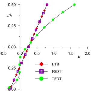
for aspect ratio 4 and 10, respectively. In case of simply supported beam, maximum uoccurs at simply supported end (x = 0 or x = L) atz = ±h / 2. The value of u given by present theory is higher by 10.21% compared to exact value. ETB and FSDT yield identical values of this dis-placement. ETB and FSDT underestimate the values by 15.56% and 3.16% for aspect ratio 4 and 10, respectively compared to exact values. The theories of Kant and Manjunatha and Lu and Liu overestimate this value by 6.40% and 3.19% respectively, for aspect ratio 4 when compared to exact values. The variation of this displacement through the thickness is graphically presented in Fig.3 and Fig.4 for aspect ratio 4 and 10 respectively, which shows the realistic variation indicat-ing the effect of shear deformation on the deformation of transverse normal.
In the case of fixed beam, maximum uoccurs at quarter span of the beam from the fixed end
support and it diminishes at fixed ends and at the middle span of the beam. The graphical presentation of this displacement is shown in Figs. 12 and 13. At quarter span (x = 0.25L) it shows considerable departure from the distributions given by ETB and FSDT at the same loca-tion. However, according to present theory, values of this displacement matches with the one given by ETB and FSDT at (x = 0.3758L) from the support for aspect ratio 4 and at (x = 0.3143L) for aspect ratio 10.
4.3 Axial stress (σ
x):
The results of maximum non-dimensional axial stress are given in Tables 1 and 2 for simply sup-ported beam subjected to sinusoidal load for aspect ratio 4 and 10, respectively. ETB and FSDT yield the identical values for this stress. ETB and FSDT underpredict axial stress value by 20.83 % and 4.51% at top compared to exact values for aspect ratio 4 and 10, respectively. The results by Kant and Manjunatha and Lu and Liu underestimate the axial stress by 2.32% and 6.94% compared to exact value for aspect ratio 4. For aspect ratio 10, Manjunatha and Kant underestimate the value by 0.605%, whereas Lu and Liu overestimate it by 0.857% compared to exact value. The distributions of this stress are shown in Figs. 5 and 6. Axial stress variation through the thickness shows the severe influence of shear deformation effect for aspect ratio 4. (see Fig.5) as compared to the variation for aspect ratio 10.
4.4 Transverse shear stresses (τ xz):
The transverse shear stresses are obtained directly by constitutive relation and, alternatively by integration of equilibrium equation of two dimensional elasticity and are denoted by (τCR
zx ) and (τEE
zx ) respectively. The transverse shear stress satisfies the stress free boundary conditions on
the top
(
z =−h/ 2)
and bottom(
z = +h/ 2)
surfaces of the beam when these stresses areob-tained by both the above mentioned approaches.
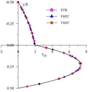
The non-dimensional transverse shear stress values for simply supported beam subjected to sinusoidal load are presented in Table 1 and 2 for aspect ratio 4 and 10 respectively. Transverse shear stress value obtained by present theory according to constitutive relation is 10.40 % higher for aspect ratio 4 and 5.63 % higher for aspect ratio 10, compared to values obtained by equilibri-um equations. The results obtained by present theory using constitutive relations are in good agreement with exact results, whereas the results obtained by equilibrium equations are in excel-lent agreement with those of exact elasticity solution. The higher order model by Maiti and Sinha underestimates the value by 10.87% compared to the exact value, whereas the value obtained by Vinayak et al. using higher order model is on higher side by 1.05% for aspect ratio 4. The through the thickness variations of this stress using constitutive relation are shown in Figs. 7 and 8. and those given by equilibrium equation are given in Figs.9 and 10.
The non-dimensional transverse shear stress values for fixed beam subjected to sinusoidal load are presented in Table 3 for aspect ratio 4 and 10. According to present theory, the transverse shear stress value by constitutive relation is 22.05 % higher for aspect ratio 4 and 20.24 % higher for aspect ratio 10 at (x = 0.2L) compared to the corresponding values obtained by equilibrium equation. ETB and FSDT yield identical values of this stress at fixed end when obtained using equilibrium equation. In case of fixed beam, through the thickness distribution of τ
zx
EE , as shown
in Figs. 18 and 19, given by present theory according to equilibrium equation shows the consider-able deviation from the distributions given by ETB and FSDT at the fixed end (x = 0) with change in sign. The maximum negative value of this stress occurred at neutral axis and maximum positive value occurred at interface (z = 0, centroidal axis). This anomalous behavior is attribut-ed to heavy local stress concentration at this end. However, this behavior can not be capturattribut-ed by use of constitutive relation. The effect of stress concentration diminishes at other locations away from the fixed end (see Figs. 18 and 19). The graphical representation of transverse shear stress using equilibrium equation shows the effect of stretching bending coupling in the bottom layer, in which fiber orientation is00
5. CONCLUSIONS
A layerwise shear deformation theory is used for the static flexural analysis of cross ply laminated (90/0) simply supported and fixed beams subjected to sinusoidal load. Euler–Bernoulli’s and Ti-moshenko’s classical theories are employed in a layerwise manner to obtain results. A general solution technique is developed for the static flexure of beams based on present theory. The re-sults by present theory for simply supported beam subjected to sinusoidal load are validated by comparing with the results by exact solution. However, the exact solution for fixed-fixed beam subjected to sinusoidal load is not available; hence results are compared with those of Euler– Bernoulli and Timoshenko classical theories. The present theory is capable to capture the effect of stress concentration at fixed end and account for the shear deformation effect in un-symmetric cross-ply laminated beams. The results obtained by present theory are in good agreement with exact elasticity solution of laminated beam. The present theory can be applied to the laminated beams with various loading and boundary conditions by developing general solution of the prob-lem.
References
[1] S. P. Timoshenko. On the Correction for Shear of the Differential Equation for Transverse Vibrations of Prismatic Bars. Philosophical Magzine, series 6(41):742-6,1921.
[2] Y. M. Ghugal and R. P. Shimpi. A review of refined shear deformation theories for isotropic and anisotropic laminated beams. Journal of Reinforced Plastics and Composites, 20(3): 255-73, 2001.
[3] J. N. Reddy. Mechanics of laminated composite plates and shells: theory and analysis. 2nd edition, Boca Raton, FL: CRC Press; 2004.
[4] I. Kreja. A literature review on computational models for laminated composite and sandwich panels. Central European Journal of Engineering, 1(1):59-80, 2011.
[5] T. Kant and B. S. Manjunatha. Refined theories for composite and sandwich beams with C0 finite elements. Computers and Structures, 33: 755-64, 1989.
[6] K. P. Soldato and P. Watson. A method for improving the stress analysis performance of one- and two-dimensional theories for laminated composites. Acta Mechanica, 123:163-86, 1997.
[7] A. M. Zenkour. Transverse shear and normal deformation theory for bending analysis of laminated and sandwich elastic beams. Mechanics of Composite Materials and Structures, 6: 267-83, 1999.
[8] B. S. Manjunatha and T. Kant. Different numerical techniques for the estimation of multiaxial stresses in symmetric/unsymmetric composite and sandwich beams with refined theories. Composite Structures, 23: 61-731993.
[9] D. K. Maiti and Sinha. Bending and Free Vibration Analysis of Shear deformable Laminated Composite Beams by Finite Element Method. Composite Structures, 29: 421-31, 1994.
[10] R. U. Vinayak, G. Pratap and B. P. Naganarayana. Beam Elements Based on a Higher Order Theory – I: Formulation and Analysis of Performance. Computers and Structures, 58: 775-89, 1996.
[11] K. H. Lo, R. M. Christensen, E. M. Wu. A Higher Order Theory for Plate Deformations, Part 1: Homogene-ous Plates. ASME journal of Applied Mechanics, 663-68, 1977.
[12] J. Park and S. Y.Lee. A new exponential plate theory for laminated composites under cylindrical bending. Transactions of theJapan SocietyforAeronautical and Space Sciences, 46 (152): 89–95, 2003.
[13] A. A. Khdeir and J. N. Reddy. An exact solution for the bending of thin and thick cross-ply laminated beams. Composite Structures, 37:195-203, 1997.
[15] D. Liu and X. Li. An overall View of Laminate Theories based on Displacement Hypothesis. Journal of Composite Materials, 30: 1539-61, 1996.
[16] X. Li and D. Liu. Zig-zag theories for composite laminates: Technical Note. AIAA Journal, 33: 1163-1165, 1995.
[17] U. Icardi. A three dimensional zig -zag theory for analysis of thick laminated beams. Composite structures, 52: 123-35, 2001.
[18] H. Arya, R. P. Shimpi and N. K. Naik. A zigzag model for laminated composite beams. Composite Struc-tures, 56:21–4, 2002.
[19] J. N. Reddy and D. H. Robbins. Theories and Computational Models for Composite Laminates. Applied Mechanics Reviews, 47:147-169, 1994.
[20] X. Lu and D. Liu. An interlaminar shear stress continuity theory for both thin and thick Laminates. ASME Journal of Applied Mechanics, 59: 502-509, 1992.
[21] A. Catapano, G. Giunta, S. Belouettar and E. Carrera. Static analysis of laminated beams via a unified formulation. Composite structures, 94(1):75-83, 2011
[22] Y. M. Ghugal and R. P. Shimpi. A new Layerwise Trigonometric Shear Deformation Theory for Two Lay-ered Cross-Ply Laminated Beams. Composites Science and Technology, 61: 1271-1283, 2001.
[23] G. M. Gere and S. P. Timoshenko. Mechanics of Materials: CBS Publishers. New Delhi. 1st Indian edition. 407- 414, 1986.
[24] Y. M. Ghugal. A two-dimensional exact elasticity solution of thick beam. Departmental report No.1. De-partment of Applied Mechanics, Government Engineering College Aurangabad, India.1-96, 2006.
Appendix
The constants Ai and Bi appeared in flexural rigidities D,D1,D2 and D3 of governing differential equations and boundary conditions [Eqs. (15) through (19)] are defined as follows:
(a) Layer 1 integration constants A1, A2, A3, A4
A 1=bh
3E(1) 1
24+ α 4+ α2 2 ⎡ ⎣ ⎢ ⎢ ⎤ ⎦ ⎥ ⎥ A
2=bh
3E(1) C 1 1 8+ α 2 ⎛ ⎝ ⎜⎜ ⎜ ⎞ ⎠ ⎟⎟ ⎟⎟+C2
1+2α π ⎛ ⎝ ⎜⎜ ⎜ ⎞ ⎠ ⎟⎟ ⎟⎟ 2
1+sin −πα 1+2α
⎛ ⎝ ⎜⎜ ⎜ ⎞ ⎠ ⎟⎟ ⎟⎟ ⎡ ⎣ ⎢ ⎢ ⎤ ⎦ ⎥ ⎥+αC2
1+2α π ⎛ ⎝ ⎜⎜ ⎜ ⎞ ⎠ ⎟⎟ ⎟⎟cos −
πα
1+2α
⎛ ⎝ ⎜⎜ ⎜ ⎞ ⎠ ⎟⎟ ⎟⎟ ⎧ ⎨ ⎪⎪⎪ ⎩ ⎪⎪ ⎪ ⎫ ⎬ ⎪⎪⎪ ⎭ ⎪⎪ ⎪ A
3=bh
3E(1) C1 2
2 −2C1C2
1+2α π ⎛ ⎝ ⎜⎜ ⎜ ⎞ ⎠ ⎟⎟ ⎟⎟cos −
πα
1+2α
⎛ ⎝ ⎜⎜ ⎜ ⎞ ⎠ ⎟⎟ ⎟⎟+ C 2 2
4 1+
1+2α π ⎛ ⎝ ⎜⎜ ⎜ ⎞ ⎠ ⎟⎟ ⎟⎟sin πα
0.5+α
⎛ ⎝ ⎜⎜ ⎜ ⎞ ⎠ ⎟⎟ ⎟⎟ ⎡ ⎣ ⎢ ⎢ ⎤ ⎦ ⎥ ⎥ ⎧ ⎨ ⎪ ⎪ ⎩ ⎪ ⎪ ⎫ ⎬ ⎪ ⎪ ⎭ ⎪ ⎪ A 4 = bhG(1) 4 C 2π 1+2α
⎛ ⎝ ⎜⎜ ⎜⎜ ⎞ ⎠ ⎟⎟ ⎟⎟ 2
1+ 1+2α
π ⎛ ⎝ ⎜⎜ ⎜ ⎞ ⎠ ⎟⎟ ⎟⎟sin −
πα
0.5+α