Topological sensitivity analysis for a two-parameter
Mooney-Rivlin hyperelastic constitutive model
Abstract
The Topological Sensitivity Analysis (TSA) is represented by a scalar function, called Topological Derivative (TD), that gives for each point of the domain the sensitivity of a given cost function when an infinitesimal hole is created. Appli-cations to the Laplace, Poisson, Helmoltz, Navier, Stokes and Navier-Stokes equations can be found in the literature. In the present work, an approximated TD expression ap-plied to nonlinear hyperelasticity using the two parameter Mooney-Rivlin constitutive model is obtained by a numeri-cal asymptotic analysis. The cost function is the total po-tential energy functional. The weak form of state equation is the constraint and the total Lagrangian formulation used. Numerical results of the presented approach are considered for hyperelastic plane problems.
Keywords
Topological Optimization, Finite Elements, Nonlinear Elas-ticity, HyperelasElas-ticity, Topological Derivative.
Carlos E. L. Pereira∗ and Marco L. Bittencourt
Department of Mechanical Design, Faculty of Mechanical Engineering, University of Camp-inas, P.O. Box 6122, CampCamp-inas, SP, 13083-970 – Brazil
Received 24 May 2010; In revised form 19 Aug 2010
∗Author email: [email protected]
1 INTRODUCTION
Topological optimization may be classified as continuous and discrete. The topological op-timization of continuous structures are given in terms of material (micro) and geometrical (macro) approaches. The main technique of the material approach is the SIMP (Solid Isotropic Microstructures with Penalization) [6]. The methods ESO (Evolutionary Structural Optimiza-tion) and TSA (Topological Sensitivity Analysis) are techniques related to the geometrical approach [25, 31, 33, 34]. For discrete structures, the optimal topology is determined by the optimal number, position and connectivity of the structural elements. A complete review of discrete topological optimization may be found in [6, 14, 17, 26, 28–30].
The TSA technique calculates the sensitivity of the cost function when an infinitesimal hole is created in the domain of the problem [8, 16, 31, 33]. The sensitivity is given by the topological derivative or gradient. In [25], the topological derivative was presented using shape sensitivity analysis and applied to the steady-state heat conduction and linear elasticity problems.
for the topological derivative in the nonlinear Helmholtz and Navier-Stokes equations have been obtained in [1–3]. Topological derivative and level set methods were presented in [7]. Applications to time dependent problems and image processing are found in [5, 22]. In [27], the TSA concept was applied to large deformation problems and an approximated expression to the topological derivative was obtained.
The purpose of this work is to extend the results obtained for large deformation with linear elastic material in [27] to nonlinear hyperelasticity using the 2 parameter Mooney-Rivlin constitutive model. In Sections 2 and 3, the topological derivative for the Lagrangian formulation and the nonlinear hyperelasticity model are reviewed. In Section 4, the expression of the topological derivative is obtained for nonlinear hyperelasticity and the total potential energy functional. In Section 5, an asymptotic numerical analysis is developed to determine the behavior of the analytical expression of the topological derivative. Finally, a heuristic topological optimization algorithm is applied to three hyperelastic two-dimensional structures and conclusions are addressed in Sections 6 and 7, respectively.
2 TSA FOR THE TOTAL LAGRANGIAN FORMULATION
The topological derivative [25] can be extended to large deformation problems using the total Lagrangian formulation as in [27]. A review of that application is presented below. It should be emphasized that this paper does not intend to present any formal proof of the topological derivative to non-linear elastic problems. The topological derivative in the cases of semilinear problem and linear elasticity is demonstrated in [19, 23], based on the asymptotic expansions which results in the topological derivatives of general shape functionals. Asymptotic analysis is also presented for nonlinear Helmholtz and Navies-Stokes equations in [1–3].
Consider a new domain Ω0
ε∈Rn, Ω
0
ε=Ω
0
−B¯ε0, that has a boundary denoted by Γ
0
ε=Γ
0
∪∂Bε0
and ¯Bε0=B
0
ε∪∂B
0
ε is a ball of radiusεand centered at the material pointXˆ ∈Ω
0
ε, as illustrated in Figure 1.
A total Lagrangian description for the topological derivative can be written as
DT(Xˆ)= lim
ε→0
δε→0
ψ(Ω0
ε+δε)−ψ(Ω
0
ε)
f(ε+δε)−f(ε) . (1)
The action of increasing the hole can be interpreted as a sequence of perturbed configu-rations characterized by the parameter τ and described by a smooth and invertible function
T (X, τ) withX∈Ω0ε⊂Rn and τ ∈R. In this way, the sequence of domains Ω0τ and respective
perturbed reference boundaries Γ0
τ can be defined as
Ω0τ ={Xτ ∈Rn∣∃ X∈Ω
0
ε,Xτ =T (X, τ),Xτ∣τ=0=X}
and Γ0
τ = {Xτ ∈Rn∣∃ X∈Γ0ε,Xτ =T (X, τ)}, where Ω0τ∣τ
=0 = Ω
0
ε and Γ
0
τ∣τ
=0 = Γ
0
ε. In this way, the domain Ω0
ε+δε, perturbed by a smooth expansion δε of the ball B
0
ε, and its respective boundary Γ0
ε+δε can be written with relation to τ as Ω
0
ε+δε =Ω
0
τ Ô⇒Ω
0
ε = Ω
0
τ∣τ
=0
and Γ0
ε+δε=Γ
0
τ Ô⇒Γ
0
ε= Γ
0
τ∣τ
=0.
The mapping between the non-perturbed reference domain Ω0
ε and the perturbed domain Ω0
τ can be written as
Xτ =X+τ Vnn0, ∀X∈∂B
0
ε, (2)
whereVn is the normal component to the hole of the velocity field Vin the reference configu-ration. The perturbationδεis associated to the parameterτ in the following way (∀ X∈ ∂B0
ε and ∀Xτ ∈∂B0
ε+δε)
δε=∥Xτ−X∥=∥τ Vnn0∥=τ∣Vn∣. (3)
Considering that the domain used in the shape variation sensitivity is the reference domain Ω0
, then the topological derivative can be rewritten as
DT(Xˆ)= 1
∣Vn∣ lim ε→0
1
f′( ε)
dψ(Ω0
τ)
dτ RRRRRRRRRRR
τ=0
, (4)
where f(ε) is the regularizing function chosen in such a way that 0<∣DT(Xˆ)∣<∞.
3 NONLINEAR HYPERELASTICITY
In a large deformation problem, the final configuration of the body Ω∈Rn can differ greatly
from the initial or reference configuration Ω0
∈ Rn. A body is deformed through a one to
one mapping f that relates each material point X ∈Ω0 to a point x ∈Ω in such a way that x=f(X)∈Ω and det∇f>0. The vector u(X)=f(X)−Xrepresents the displacement of the
material point X.
For a homogeneous incompressible hyperelastic material, the constitutive equation is given by [18]
where p∈Ris the Lagrange multiplier related to the hydrostatic pressure andJ =detF.
Following [10], the strain energy density functionalW for an isotropic hyperelastic material may be decomposed as the sum of the distortional ( ¯W) and the volumetric ˜W strain energy densities as
W(I¯1,I¯2, I3)=W¯ (I¯1,I¯2)+W˜ (I3), (6)
where ¯I1=I1I− 1/3
3 , ¯I2=I2I− 2/3
3 and I3=detCis the third invariant of the right Cauchy-Green
deformation tensor C. In addition, the following equation relates the hydrostatic pressure p
and the volumetric strain energy density ˜W [10]
p= ∂W˜ (I3)
∂J . (7)
In this work, the distortional and volumetric densities are written in terms of the Mooney-Rivlin form with two-parameters, respectively, as [9–12, 21]
¯
W(I¯1,I¯2)=A10(I¯1−3)+A01(I¯2−3), (8)
˜
W(I3)=
˜
k
2(J−1)
2
, (9)
where A10 and A01 are material constants and ˜kis the bulk modulus, which is a numerical
penalization term for nearly incompressible materials. After replacing equations (8) and (9) in (6), the strain energy density functional for an isotropic nearly incompressible hyperelastic material is given by
W(I¯1,I¯2, J)=A10(I¯1−3)+A01(I¯2−3)+
˜
k
2(J−1)
2
, (10)
The mixed variational form of the non-linear nearly incompressible hyperelastic problem is expressed by: findu∈U and p∈Q such that [32]
{ a(u, δu)+b1(δu, p)=l(δu) ∀δu∈V
b2(u, δp)−g(p, δp)=0 ∀δp∈Q
, (11)
with
a(u, δu) = ∫ Ω0[
∂W¯ ∂I¯1
∂I¯1
∂E +
∂W¯ ∂I¯2
∂I¯2
∂E]⋅δEdΩ 0
= ∫Ω0
¯
S⋅δEdΩ0, (12)
b1(δu, p) = ∫ Ω0p
∂J
∂E ⋅δEdΩ 0
= ∫Ω0
˜
S⋅δEdΩ0, (13)
b2(u, δp) = ∫ Ω0(J(
u)−1)δp dΩ0, (14)
g(p, δp) = ∫
Ω0
p
˜
kδp dΩ
0
, (15)
l(δu) = ∫ Ω0
b0⋅δudΩ
0
+∫
Γ0
N
t0⋅δudΓ 0
where U ={u∈[H1(Ω0)]dim∣u∣Γ0
D =
¯
u} with dim ≤3 and Q ={p∈L2(Ω 0
)}. It is assumed that the reference domain Ω0
∈ Rn is open and bounded. Its boundary Γ0 = Γ0N ∪Γ0
D
(Γ0
D∩Γ
0
N =∅)is sufficiently regular and admits the existence of a normal unitary vectorn in almost all of the points of Γ0
, except in a finite set of zero measure.
4 TSA IN NONLINEAR HYPERELASTIC PROBLEMS
In this section, the expression of the topological derivative for the isotropic nearly incom-pressible hyperelastic problem is obtained from equation (1). This expression requires the evaluation of a given cost function Ψ, defined on the non-deformed configuration Ω0
ε, when the hole Bε0 centered in X ∈Ω
0
ε and ε→0 increases in size according to the velocity field defined. The topological derivative is related to the shape sensitivity analysis as indicated in equation (4).
The mixed variational statement for the elastic problem with large deformation and ho-mogeneous, isotropic and nearly incompressible hyperelastic material in the reference non-perturbed domain Ω0
ε, assuming that the domain Ω
0
ε is limited and open and Γ
0
ε sufficiently regular, is given by: find uε∈Uε and pε∈Qε such that
{ aε(uε, δuε)+b1ε(δuε, pε)=lε(δuε) ∀δuε∈Vε
b2ε(uε, δpε)−gε(pε, δpε)=0 ∀δpε∈Qε
, (17)
where Uε, Vε and Qε are, respectively, the spaces of the admissible kinematically functions, their variations and pressures defined on the reference domain with the non-perturbed hole
Bε.
An equivalent mixed variational problem to the system given in (17) in the non-perturbed reference domain Ω0
ε may be defined by the family of perturbed reference domains Ω
0
τ, remem-bering that Ω0
τ∣τ
=0=Ω
0
ε, as: find uτ ∈Uτ and pτ ∈Qτ such that
{ aτ(uτ, δuτ)+b1τ(δuτ, pτ)=lτ(δuτ) ∀ δuτ ∈Vτ, ∀τ ≥0
b2τ(uτ, δpτ)−gτ(pτ, δpτ)=0 ∀ δpτ ∈Qτ, ∀τ ≥0
, (18)
whereUτ,Vτ andQτ are the spaces of kinematically admissible functions, their variations and pressures defined in Ω0
τ, respectively.
Considering the strain energy functional per unit of non-deformed volume given in (10), the total potential energy functional Ψτ(uτ) is written in Ω0τ as
Ψτ(uτ)= ∫ Ω0
τ
W(I¯1τ,I¯2τ, Jτ)dΩ
0
τ −∫
Ω0
τ
b0⋅uτ dΩ
0
τ −∫
Γ0
N
t0⋅uτ dΓ
0
τ . (19)
To obtain the sensitivity of the cost function (19), the lagrangian function for the hypere-lastic problem, in the non-perturbed configuration Ω0
τ, is written as
Lτ(uτ, βτ, pτ, θτ) = Ψτ(uτ)+aτ(uτ, βτ)+b1τ(βτ, pτ)
where βτ =m1δuτ and θτ =m2δpτ (m1 and m2∈R) are, respectively, the Lagrange
multi-pliers related to the first and second equations of the mixed variational system (18). However, considering that equation (18) is satisfied for all τ, the derivative of the lagrangian function (20) will be the same as the derivative of the total potential energy functional
dLτ
dτ = dΨτ
dτ = ∂Lτ
∂τ +⟨ ∂Lτ
∂uτ,u˙τ⟩+⟨
∂Lτ
∂βτ
,β˙τ⟩+⟨
∂Lτ
∂pτ
,p˙τ⟩+⟨
∂Lτ
∂θτ
,θ˙τ⟩, (21)
where u˙τ = duτ
dτ ∈Vτ,
˙
βτ = dβdττ ∈Vτ, ˙pτ = dpdττ ∈Qτ and ˙θτ = dθdττ ∈Qτ. The directional derivatives in (21) are given, respectively, by
⟨∂aτ
∂uτ,u˙τ⟩ = ∫Ω0
τ
C(uτ)∶⟨∂Eτ
∂uτ,u˙τ⟩⋅δEτ
+ Sτ⋅⟨∂δEτ
∂uτ ,u˙τ⟩dΩ 0
τ =δaτ(sτ;u˙τ, βτ), (22)
⟨∂aτ
∂βτ
,β˙τ⟩= ∫
Ω0
τ
¯
Sτ ⋅⟨∂Eτ
∂uτ, ˙
βτ⟩dΩ
0
τ =aτ(uτ,β˙τ), (23)
⟨∂b1τ
∂βτ
,β˙τ⟩= ∫
Ω0
τ
˜
Sτ⋅⟨∂Eτ
∂uτ, ˙
βτ⟩dΩ
0
τ =b1τ(β˙τ, pτ), (24)
⟨∂b1τ
∂pτ
,p˙τ⟩= ∫
Ω0
τ
˙
pτ
∂J(uτ)
∂Eτ ⋅⟨
∂Eτ
∂uτ, βτ⟩dΩ 0
τ =δb1τ(sτ;βτ,p˙τ), (25)
⟨∂b2τ
∂uτ ,u˙τ⟩= ∫Ω0
τ
∂J(uτ)
∂Eτ ⋅⟨
∂Eτ
∂uτ,u˙τ⟩θτ dΩ 0
τ =δb2τ(sτ;u˙τ, θτ), (26)
⟨∂b2τ
∂θτ
,θ˙τ⟩= ∫
Ω0
τ
[J(uτ)−1]θ˙τ dΩ
0
τ =b2τ(uτ,θ˙τ), (27)
⟨∂gτ
∂pτ
,p˙τ⟩= ∫
Ω0
τ
˙
pτ ˜
k θτ dΩ
0
τ =δgτ(pτ; ˙pτ, θτ), (28)
⟨∂gτ
∂θτ
,θ˙τ⟩= ∫
Ω0 τ pτ ˜ k ˙
θτ dΩ
0
τ =gτ(pτ,θ˙τ), (29)
⟨∂lτ
∂βτ
,β˙τ⟩= ∫
Ωτ
b0⋅β˙τ dΩ
0
τ −∫
ΓN
t0⋅β˙τ dΓ
0
τ =lτ(β˙τ). (30)
The partial derivative of the lagrangian function (20) inτ is the same as the total derivative if the directional derivatives presented in (21) are zero. Therefore, from (22) to (30), the following variational problem is obtained: find uτ ∈Uτ and pτ ∈Qτ such that
{ aτ(uτ,β˙τ)+b1τ(β˙τ, pτ)=lτ(β˙τ) ∀β˙τ ∈Vτ, ∀τ ≥0
b2τ(uτ,θ˙τ)−gτ(pτ,θ˙τ)=0 ∀θ˙τ ∈Qτ, ∀τ ≥0
which represents the state equation for the considered problem. The adjoint problem is: find
βτ ∈Vτ and θτ ∈Qτ such that
⎧⎪⎪ ⎨⎪⎪ ⎩
δaτ(sτ;βτ,u˙τ)+δb2τ(sτ;u˙τ, θτ)=−⟨∂
Ψτ
∂uτ,
˙
uτ⟩ ∀u˙τ ∈Vτ, ∀τ ≥0
δb1τ(sτ;βτ,p˙τ)−δgτ(pτ;θτ,p˙τ)=0 ∀p˙τ ∈Qτ, ∀τ ≥0
, (32)
where the symmetry of the bilinear forms δaτ(sτ;u˙τ, βτ) and δgτ(pτ; ˙pτ, θτ) has been taken into account.
The directional derivative of the total potential energy functional inuτ in the directionu˙τ,
according to (19), may be written as
⟨∂∂Ψτu
τ
,u˙τ⟩ = ∫ Ω0
τ
(∂Wτ
∂I¯1τ
∂I¯1τ
∂Eτ +
∂Wτ
∂I¯2τ
∂I¯2τ
∂Eτ +
∂Wτ
∂Jτ
∂Jτ
∂Eτ)⋅⟨
∂Eτ
∂uτ,u˙τ⟩dΩ 0
τ
−∫
Ω0
τ
b0⋅u˙τ dΩ
0
τ −∫
Γ0
N
t0⋅u˙τ dΓ
0
τ ,
⟨∂∂Ψτu
τ
,u˙τ⟩ = aτ(uτ,u˙τ)+b1τ(u˙τ, pτ)−lτ(u˙τ)=0 ∀u˙τ ∈Vτ, ∀τ ≥0, (33)
where it has been assumed that uτ and pτ satisfy the state equation (18). Consequently, the solution of the adjoint equation (32) is (βτ, θτ) =(0,0) and the partial derivative of the lagrangian (20), written in the perturbed configuration Ω0
τ, is
∂Lτ
∂τ ∣τ=0
= ∂Ψτ(uτ)
∂τ ∣τ
=0
= ∂
∂τ ∫Ω0
τ
W(Eτ)dΩ0
τ∣ τ=0
− ∂lτ(uτ)
∂τ ∣τ
=0
. (34)
Replacing the definition of the total potential energy for the non-linear nearly incompress-ible hyperelastic problem, given in (19), in (34) and using the Reynolds Transport Theorem, the partial derivative of the lagrangian function in the non-perturbed configuration Ω0
τ∣τ
=0=Ω
0
ε is given by
∂Lτ
∂τ ∣τ=0= ∫Ω
0
ε
∂W(Eτ)
∂τ ∣τ
=0
+W(Eε)DivVdΩ0
ε −
∂lτ(uτ)
∂τ ∣τ
=0
, (35)
where
∂lτ(uτ)
∂τ ∣τ
=0
= ∫Ω0
ε
(b0⋅uε)I⋅ ∇VdΩ0ε (36)
foruτ and βτ fixed and the velocity field V defined by
{ V= Vnn0 withVn<0 and constant on ∂Bε0
V=0 on Γ0
considering Γ0
ε=Γ
0
∪∂B0
ε
, (37)
Therefore, equation (35) is rewritten as
∂Lτ
∂τ ∣τ=0= ∫Ω
0
ε
Sτ ⋅∂Eτ
∂τ ∣τ=0
dΩ0ε +∫
Ω0
ε
[(W(Eε)−b0⋅uε)]I⋅ ∇VdΩ
0
where
∂Eτ
∂τ ∣τ=0
= ∂(∇τuSτ)
∂τ RRRRRRRRRR
Rτ=0
+1
2
∂(∇τuTτ)
∂τ RRRRRRRRRR
Rτ=0
∇uτ+1
2∇u T τ
∂(∇τuτ)
∂τ ∣τ
=0
. (39)
Using the definition of the partial derivative of the Green-Lagrange strain tensor Eτ in
the non-perturbed configuration Ω0
ε, given in (39), equation (38), after a few manipulations, becomes
∂Lτ
∂τ ∣τ=0= ∫Ω0ε
{[W(Eε)−b0⋅uε]I− ∇uεTSε− ∇uTε∇uεSε}⋅ ∇VdΩ
0
ε. (40)
Equation (40) may be expressed in the following form
∂Lτ
∂τ ∣τ=0= ∫Ω
0
ε
Σ0ε⋅ ∇VdΩ0ε, (41)
whereΣ0ε is the Eshelby’s energy moment tensor in the non-perturbed reference configuration
Ω0
ε for the total lagrangian formulation [15]. For the considered problem, it is defined by
Σ0ε =[W(Eε)−b0⋅uε]I− ∇uTεSε− ∇uTε∇uεSε. (42)
or in terms of the first Piola-Kirchhoff tensor
Σ0ε =[W(Eε)−b0⋅uε]I− ∇uTεPε. (43)
From the divergence theorem and the tensorial expression
Σ0ε⋅ ∇V=Div[(Σ0ε)TV]−Div(Σ0ε)⋅V, (44)
equation (41) is rewritten as
∂Lτ
∂τ ∣τ=0= ∫Ω0ε
Div(Σ0
ε)⋅VdΩ
0
ε +∫
Γ0
ε
Σ0
εn0⋅VdΓ 0
ε. (45)
It is possible to show that
DivΣ0ε =0. (46)
Replacing equation (46) in (45) and considering the velocity field (37), the following equa-tion is obtained
∂Lτ
∂τ ∣τ=0
=−Vn∫ ∂B0
ε
Σ0
εn0⋅n0d∂B 0
ε . (47)
From the definition of the Eshelby’s tensor Σ0
ε given in (43), the following relation is valid
Σ0εn0⋅n0=W(Eε)−b0⋅uε−Pεn0⋅(∇uε)n0.
Considering a homogeneous Neumann boundary condition in the hole, i.e., Pεn0 =0 on
∂Bε0, and no body forces, b0 = 0, the partial derivative of the lagrangian function in τ = 0
becomes
∂Lτ
∂τ ∣τ=0
=−Vn∫ ∂B0
ε
The topological derivative, except for the limit ε→0, is obtained after the substitution of (48) in the expression of the topological derivative for the total lagrangian formulation given in (4). Therefore,
DT(Xˆ)=−lim ε→0
1
f′(ε)∫
∂B0
ε
W(Eε)d∂Bε0. (49)
5 NUMERICAL ASYMPTOTIC ANALYSIS
Equation (49) represents the topological derivative, except for the limit with ε→ 0, for the
case of large deformations and nonlinear nearly incompressible hyperelasticity. In order to obtain the topological derivative, it is necessary that the limit for ε→0 in (49) be calculated
either analytical or approximately. For the present non-linear problem, an analytic asymptotic analysis of equation (49) becomes impracticable. A procedure based on numerical experiments for the calculation of the limit with ε→0 in (49) was used in [27] for large deformation and
linear elastic material. The same asymptotic analysis is applied below to large deformation and Mooney-Rivlin material.
The topological sensitivity analysis aims to provide an asymptotic expansion of a shape functional with respect to the size of a small hole created inside the domain [3]. The asymptotic analysis makes possible to obtain the behavior of the integrand of the topological derivative expression (49) in the limit when the hole radius becomes small. Another point is to compare the quotient between the topological derivative in the domain with a small hole and the strain energy functional in the domain without the hole.
Consider the function dT(uε) defined by
dT(uε)=− 1
f′(ε)∫
∂B0
ε
W(Eε)d∂Bε0, (50)
in such a way that
DT(Xˆ)=lim ε→0dT(
uε). (51)
A numerical study of the asymptotic behavior of the function dT(uε) with relation to the radiusε is developed.
Consider a plane square domain, denoted by Ω, with sizeL=2mmand a hole of radiusε
at the center of the domain, subjected to the distributed load casest0along the edges of Ω, as
illustrated in Figure 2. It is assumed plane strain and Mooney-Rivlin model with A10 =0.55
N/mm2, A01 = 0.138 N/mm 2
(a) First case model. (b) Second case model.
(c) Third case model. (d) Fourth case model.
Figure 2 Models used in the asymptotic analysis [27].
(a) Mesh without hole. (b) Mesh with hole ε = 0.16 mm.
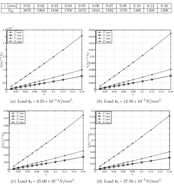
The finite element meshes of quadratic triangles are constructed in such a way that they have the same number of elements at the boundary of the hole, independently of the value of the radius ε. Consequently, the approximated size of the elements is calculated as
he≈ 2πε ne
, (52)
being ne the number of elements required over the boundary of the hole. Table 1 shows the total number of elements NE of the meshes generated in the domain Ω for different values of the radius εand ne=60.
Table 1 Meshes used in the numerical asymptotic analysis.
ε[mm] 0.01 0.02 0.03 0.04 0.05 0.06 0.07 0.08 0.10 0.12 0.16
NE 3876 1968 1846 1760 1672 1644 1592 1576 1480 1408 1296
0 0.02 0.04 0.06 0.08 0.1 0.12 0.14 0.16 0 0.5 1 1.5 2 2.5 3 3.5 4 4.5x 10
−3
ε dT
(uε
) * f
,(u ε ) 1º case 2º case 3º case 4º case
(a) Loadt0=6.25×10− 3
N/mm2.
0 0.02 0.04 0.06 0.08 0.1 0.12 0.14 0.16 0 0.002 0.004 0.006 0.008 0.01 0.012 0.014 0.016 0.018 ε dT (uε
) * f
,(u ε ) 1º case 2º case 3º case 4º case
(b) Loadt0=12.50×10− 3
N/mm2.
0 0.02 0.04 0.06 0.08 0.1 0.12 0.14 0.16 0 0.01 0.02 0.03 0.04 0.05 0.06 0.07 0.08 ε dT (uε
) * f
,(u ε ) 1º case 2º case 3º case 4º case
(c) Loadt0=25.00×10− 3
N/mm2.
0 0.02 0.04 0.06 0.08 0.1 0.12 0.14 0.16 0 0.02 0.04 0.06 0.08 0.1 0.12 0.14 0.16 0.18 0.2 ε dT (uε
) * f
,(u ε ) 1º case 2º case 3º case 4º case
(d) Loadt0=37.50×10− 3
N/mm2.
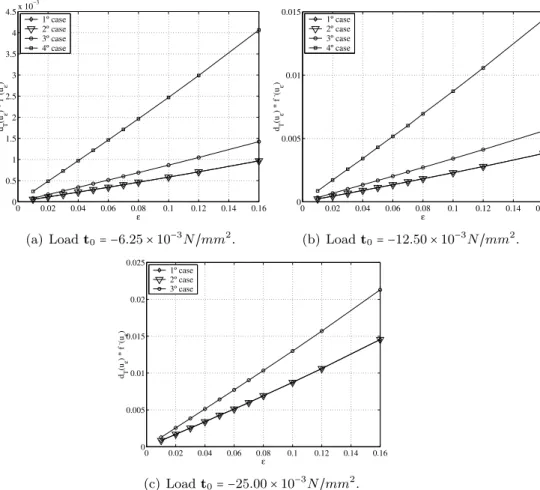
Figure 4 Asymptotic behavior ofdT(uε)f
′
The plots of the asymptotic behavior of dT(uε)f
′
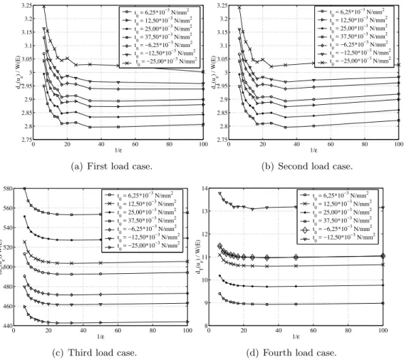
(ε)×ε are shown in Figures 4 and 5, respectively, for the traction loads t0 = {6.25; 12.50; 25.00; 37.50}×10−3
N/mm2
and com-pression loads t0 = −{6,25; 12,50; 25,00}×10−3 N/mm2 loads. Based on these results, it is
reasonable to assume that the integrand term in equation (50) behaves as a straight line trough the origin in relation to ε. A functionf(ϵ) which satisfies the condition 0<∣DT(Xˆ)∣<∞ is
f(ε)=−∣Bε∣=−πε
2
. Consequently, equations (50) and (51) give
DT(Xˆ)=lim ε→0
dT(uε)=CW(E). (53)
0 0.02 0.04 0.06 0.08 0.1 0.12 0.14 0.16 0
0.5 1 1.5 2 2.5 3 3.5 4 4.5x 10
−3
ε dT
(uε
) * f
,(u
ε
)
1º case 2º case 3º case 4º case
(a) Loadt0= −6.25×10− 3
N/mm2
.
0 0.02 0.04 0.06 0.08 0.1 0.12 0.14 0.16 0
0.005 0.01 0.015
ε
dT
(uε
) * f
,(u
ε
)
1º case 2º case 3º case 4º case
(b) Loadt0= −12.50×10− 3
N/mm2
.
0 0.02 0.04 0.06 0.08 0.1 0.12 0.14 0.16 0
0.005 0.01 0.015 0.02 0.025
ε dT
(uε
) * f
,(u
ε
)
1º case 2º case 3º case
(c) Loadt0= −25.00×10− 3
N/mm2.
Figure 5 Asymptotic behavior ofdT(uε)f
′
(ε)in terms of the radiusεfor the compression non-linear hyper-elastic problem.
The analysis of the constantCis based on the asymptotic behavior of the function dT(uε) in relation to the radius ε. For that purpose, consider the quotient between the function
holes (see Figure 3). Therefore, for f(ε)=−πε2
, the following quotient is obtained
1
2πε∫
∂B0
ε
W(Eε)d∂B0
ε
W(E) . (54)
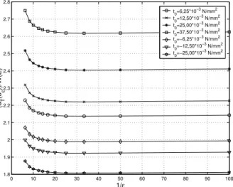
The plots in Figure 6 show the behavior of this quotient versus 1/ε for each value of t0 and
the four load cases. The plots for the first, second and fourth load cases miss a certain smoothness and have an increase in the quotient forε=0.01 (1ε =100). This behavior may be related to the distortion of the elements around the hole which is amplified as the values oft0
increase. In the compressive case, this point was much more critical and made impossible to run the simulations for the case witht0≤−25.00×10⁻³N/mm2. However, it seems reasonable
to assume an asymptotic behavior of equation (54), in function of ε, for all traction and compression load cases.
0 20 40 60 80 100
2.75 2.8 2.85 2.9 2.95 3 3.05 3.1 3.15 3.2 3.25 1/ε dT (uε
) / W(E)
t 0 = 6,25*10
−3 N/mm2 t
0 = 12,50*10 −3 N/mm2 t
0 = 25,00*10 −3 N/mm2 t
0 = 37,50*10 −3 N/mm2 t
0 = −6,25*10 −3 N/mm2 t
0 = −12,50*10 −3 N/mm2 t
0 = −25,00*10 −3 N/mm2
(a) First load case.
0 20 40 60 80 100
2.75 2.8 2.85 2.9 2.95 3 3.05 3.1 3.15 3.2 3.25 1/ε dT (uε
) / W(E)
t 0 = 6,25*10
−3 N/mm2 t
0 = 12,50*10 −3 N/mm2 t
0 = 25,00*10 −3 N/mm2 t
0 = 37,50*10 −3 N/mm2 t
0 = −6,25*10 −3 N/mm2 t
0 = −12,50*10 −3 N/mm2 t
0 = −25,00*10 −3 N/mm2
(b) Second load case.
0 20 40 60 80 100
440 460 480 500 520 540 560 580 1/ε (dT (uε ))/W(E) t 0 = 6,25*10
−3 N/mm2 t
0 = 12,50*10 −3
N/mm2 t0 = 25,00*10−3 N/mm2 t
0 = 37,50*10 −3
N/mm2 t
0 = −6,25*10 −3
N/mm2 t0 = −12,50*10−3 N/mm2 t
0 = −25,00*10 −3
N/mm2
(c) Third load case.
0 20 40 60 80 100
8 9 10 11 12 13 14 1/ε dT (uε
) / W(E)
t 0 = 6,25*10
−3 N/mm2 t
0 = 12,50*10 −3
N/mm2 t0 = 25,00*10−3 N/mm2 t
0 = 37,50*10 −3
N/mm2 t
0 = −6,25*10 −3
N/mm2 t
0 = −12,50*10 −3
N/mm2
(d) Fourth load case.
Figure 6 Asymptotic behavior of the quotient dT(uε)
W(E) in relation to the radiusεfor the non-linear hyperelastic
For the third load case, the values for C are much larger than for the other load cases. The C values depend on the combination of loads and material properties. For the third load case,C is larger because the strain energy density calculated on the central node of the mesh without hole (denominator of equation (54)) is very small. The distortional strain energy is almost zero. Due to the near-incompressibility behavior of the Mooney-Rivlin material, the volumetric part is also very small. Figure 7 shows the results for the third load case with ˜
k=1.0N/mm2 which makes the material more compressible. The values forC are now much smaller and close to the values obtained for the linear elastic material given in [27]. However, the main point of the asymptotic analysis is that the variation range of theC values is more limited than the strain energy densities W for a given load and material properties.
0 10 20 30 40 50 60 70 80 90 100
1.8 1.9 2 2.1 2.2 2.3 2.4 2.5 2.6 2.7 2.8
1/ε
(dT (uε
))/W(E)
t
0=6,25*10 −3 N/mm2
t
0=12,50*10 −3 N/mm2
t0=25,00*10−3 N/mm2 t0=37,50*10−3 N/mm2 t
0=−6,25*10 −3 N/mm2
t
0=−12,50*10 −3 N/mm2
t0=−25,00*10−3 N/mm2
Figure 7 Asymptotic behavior of the quotient dT(uε)
W(E) in relation to the radiusεfor the third load case and
˜
k=1.0N/mm2.
Table 2 Analysis of the variation of the constantCfor the first traction load case in the nearly incompressible hyperelastic problem.
t0(N/mm
2
) 0.00625 0.0125 0.025 0.0375
W(N mm/mm3
) 0.000327 0.001353 0.005696 0.013592
C 2.99 2.87 2.84 2.80
Table 3 Analysis of the variation of the constantCfor the second traction load case in the nearly incompressible hyperelastic problem.
t0(N/mm
2
) 0.00625 0.0125 0.025 0.0375
W(N mm/mm3) 0.000327 0.001354 0.005699 0.013597
C 2.99 2.87 2.84 2.80
Table 4 Analysis of the variation of the constantCfor the third traction load case in the nearly incompressible hyperelastic problem.
t0(N/mm
2
) 0.00625 0.0125 0.025 0.0375
W(N mm/mm3) 0.000003 0.000012 0.000046 0.000104
C 495.00 515.00 530.00 555.00
Table 5 Analysis of the variation of the constantCfor the fourth traction load case in the nearly incompressible hyperelastic problem.
t0(N/mm
2
) 0.00625 0.0125 0.025 0.0375
W(N mm/mm3
) 0.000353 0.001522 0.007251 0.019504
C 11.00 10.70 9.80 9.00
strain energy density is much larger when compared to the variation ofCfor all the considered cases.
Based on the previous results, the expression of the topological derivative for the non-linear nearly incompressible hyperelastic problem may be written approximately as
DT(Xˆ)≈C∗W(E), (55)
whereC∗ is taken from the previous values obtained forC. The effective value of the constant
C∗ becomes of little practical interest, because the topological derivative will be calculated for all the nodes of the mesh and the holes will be created where the topological derivative assumes the least values [27].
6 RESULTS
In this section, the heuristic algorithm used in [27] is applied to obtain the topology of three two-dimensional non-linear hyperelastic large deformation problems.
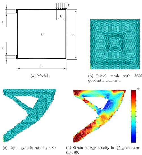
6.1 Clamped short beam
In this example, the initial domain is a square modeled as plane strain problem with sides
L=50 mm, Mooney-Rivlin constantsA10=0.55 N/mm2,A01=0.138N/mm2and ˜k=666.66
N/mm2. The beam is clamped on the regions indicated by a= 5 mm and subjected to the distributed load t0=−0.4444N/mm
2
on the region indicated byb=4.5 mm, as illustrated in Figure 8(a).
A mesh of 3656 triangular quadratic finite elements showed in Figure 8(b) was used. The stopping criterion was based on the final area ¯A=0.40A0, withA0the initial domain area, and
(a) Model. (b) Initial mesh with 3656 quadratic elements.
(c) Topology at iterationj=89.
1 2 3 4 5 6 7 8 9 x 10⁻³
(d) Strain energy density in N mm
mm3 at
itera-tion 89.
Figure 8 Clamped short beam under non-linear nearly incompressible hyperelasticity.
0 10 20 30 40 50 60 70 80 90 −6
−5.5 −5 −4.5 −4 −3.5 −3 −2.5
Iterations
Ψ
(u)
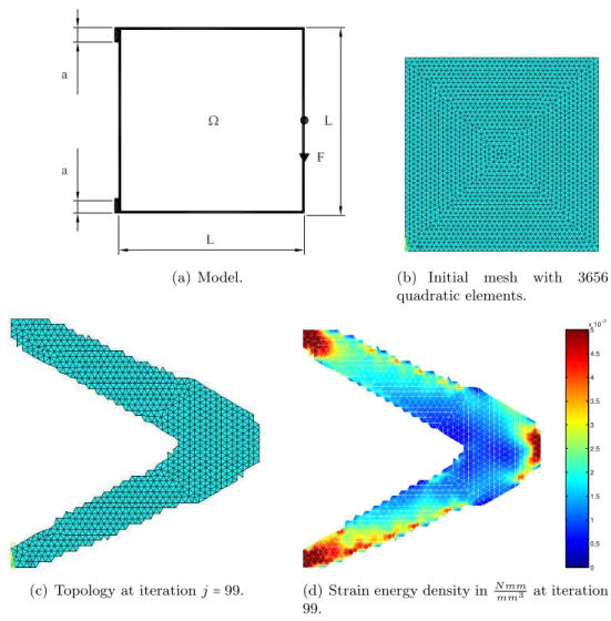
6.2 Two bars
In this example, the initial domain is subjected to a concentrated loadF =−1.0N as illustrated in Figure 10(a). The other parameters are the same used in the previous example. The required final area is ¯V =0.36V0. The final topology, illustrated in Figure 10(c), is achieved after 99
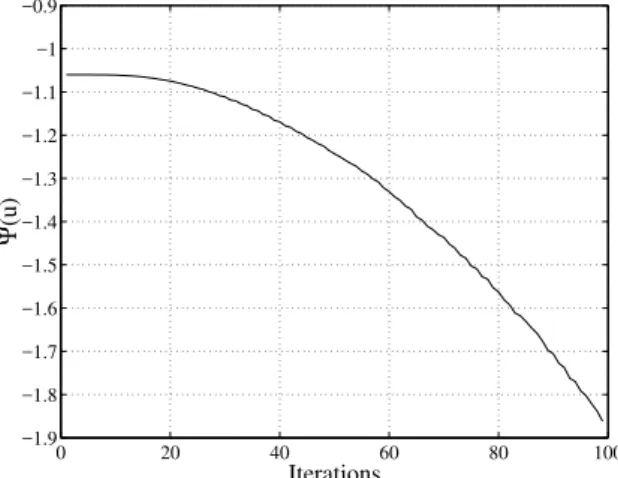
iterations and the maximum deflexion is −3.75 mm on the point of load application. Figure 10(d) illustrates the behavior of the total potential energy functional along the iterations of the algorithm. Figure 11 shows the distribution of the strain energy densityW on the domain after 99 iterations.
(a) Model. (b) Initial mesh with 3656
quadratic elements.
(c) Topology at iterationj=99.
0 0.5 1 1.5 2 2.5 3 3.5 4 4.5 5 x 10⁻³
(d) Strain energy density in N mm
mm3 at iteration
99.
0 20 40 60 80 100 −1.9
−1.8 −1.7 −1.6 −1.5 −1.4 −1.3 −1.2 −1.1 −1 −0.9
Iterations
Ψ
(u)
Figure 11 Total potential energy versus iteration number.
6.3 Clamped-clamped short beam
In this third example, the clamped-clamped beam given in Figure 12 is considered for L=20
mm and a concentrated forceF =−0.04 N applied on the beam middle span. The same pre-vious material constants are used. The final considered area is ¯V =0.20V0 and the percentage
of removed area is 3% for each iteration. The final topology is obtained after 52 iterations and illustrated in Figure 13(b). A similar result was obtained in [20, 27] for large deformation and linear elastic material.
Figure 12 Clamped-clamped beam.
7 CONCLUSIONS
This paper presented the application of the TSA to large deformation and nearly incompressible hyperlastic Mooney-Rivlin material using the total Lagrangian formulation.
(a) Initial mesh with 2302 quadratic elements. (b) Topology at iterationj=42.
0.5 1 1.5 2 2.5 3 3.5 4 4.5 x 10⁻³
(c) Strain energy density in N mm
mm3 at iteration 42.
0 5 10 15 20 25 30 35 40 45
−0.045 −0.04 −0.035 −0.03 −0.025 −0.02 −0.015 −0.01
Iterations
Ψ
(u)
(d) Total potential energy versus iteration number.
Figure 13 Clamped-clamped beam example under non-linear nearly incompressible hyperelasticity.
materials.
A heuristic topological optimization algorithm was applied to three planar problems with deformation of about 20%. In the case of the third example, similar topologies were obtained with those ones calculated using large deformation and linear material [27].
Most of the computational cost is related to the solution of the state equation due to the nearly incompressible material model and the possibility of the locking phenomenon. Once the solution has converged, the topological derivative is given by the strain energy functional as indicated in expression (55).
The final solution in Figure 13(b) shows the formation of mechanisms. This is related to the way the optimization algorithm is implemented based on the removal of a fixed amount of material. In this sense, the implemented TSA procedure has the same limitations of most hard-kill methods.
Originally, the TSA approach did not define a classical minimization problem. In [4], the topological derivative is used as a descent direction in the optimization problem. Also a penalty method is used for the constraint imposition in terms of the von Mises stress.
References
[1] S. Amstutz. The topological asymptotic for the Helmholtz equation. SIAM Journal on Control and Optimization,
42(5):1523–1544, 2003.
[2] S. Amstutz. The topological asymptotic for the Navier-Stokes equations.ESAIM: Control, Optimisation and Calculus
of Variations, 11(3):401–425, 2005.
[3] S. Amstutz. Topological sensitivity analysis for some nonlinear PDE systems. Journal de Math´ematiques Pures et
Appliqu´ees, 85(4):540–557, 2006.
[4] S. Amstutz and A.A. Novotny. Topological optimization of structures subject to von mises stress constraints.
Struc-tural and Multidisciplinary Optimization Journal, 41(3):407–420, 2010.
[5] S. Amstutz, T. Takahashi, and B. Vexler. Topological sensitivity analysis for time-dependent problems. ESAIM:
Control, Optimisation and Calculus of Variations, 14(3):427–455, 2008.
[6] M. P. Bendsφe. Optimization of Structural Topology, Shape and Material. Springer, Heidelberg, 1995.
[7] M. Burger, B. Hackl, and W. Ring. Incorporating topological derivatives into level set methods. Journal of
Compu-tational Physics, 194(1):344–362, 2004.
[8] J. C´ea, Ph. Guillaume, and M. Masmoudi. The shape and topological optimizations connection. Technical Report,
UFR MIG, Universit´e Paul Sabatier, Toulouse, French, 1998.
[9] J.S. Chen, W. Han, C.T. Wu, and W. Duan. On the perturbed lagrangian formulation for nearly incompressible and
incompressible hyperelasticity. Computer Methods in Applied Mechanics and Engineering, 142:335–351, 1997.
[10] J.S. Chen and C. Pan. A pressure projection method for nearly incompressible rubber hyperelasticity, Part I: Theory.
Journal of Applied Mechanics, 63:862–868, 1996.
[11] J.S. Chen, C.T. Wu, and C. Pan. A pressure projection method for nearly incompressible rubber hyperelasticity,
part II: Applications. Journal of Applied Mechanics, 63:869–876, 1996.
[12] J.S. Chen, S. Yoon, H.P. Wang, and W. K. Liu. An improved reproducing kernel particle method for nearly
incom-pressible finite elasticity. Computer Methods in Applied Mechanics and Engineering, 181:117–145, 2000.
[13] J. Rocha de Faria, A.A. Novotny, R.A. Feijo, and E. Taroco. First and second order topological sensitivity analysis
for inclusions.Inverse Problems in Science and Engineering Journal, 17(5):665–679, 2009.
[14] H. Eschenauer, N. Olhoff, and (eds). Optimization methods in structural design. In EUROMECH-Colloquium,
volume 164, Wien, 1982. B.I.-Wissenschaftsverlag.
[15] J. D. Eshelby. The elastic energy-momentum tensor. Journal of Elasticity, 5(3-4):321–335, April 1975.
[16] S. Garreau, Ph. Guillaume, and M. Masmoudi. The topological gradient. Technical Report, Universit´e Paul Sabatier,
Toulouse, French, 1998.
[17] W. Gutkowski and Z. Mroz. Second world congress of structural and multidisciplinary optimization. InWCSMO-2,
Intitute of Fundamental Technological Research, volume 182, Warsaw, Poland, 1997.
[18] G. A. Holzapfel. Nonlinear Solid Mechanics: A Continuum Approach for Engineering. John Wiley & Sons, 2000.
[19] M. Iguernane, S.A. Nazarov, J.-R. Roche, J. Sokolowski, and K. Szulc. Topological derivatives for semilinear elliptic
equations. Appl. Math. Comput. Sci., 19(2):191–205, 2009.
[20] D. Jung and C. Gea. Topology optimization of nonlinear structures.Finite Elements in Analysis and Design, 40:1417
– 1427, 2004.
[21] N. H. Kim. Shape Design Sensitivity Analysis and Optimization of Nonlinear Static/Dynamic Structures with
Contact/Impact. PhD thesis, The University of Iowa, May 1999.
[22] I. Larrabide, R.A. Feij´oo, A.A. Novotny, E. Taroco, and M. Masmoudi. Topological derivative: A tool for image
processing. Computers & Structures, 86:1386–1403, 2005.
[23] S.A. Nazarov and J. Soko lowski. Asymptotic analysis of shape functionals. Journal de Math´ematiques Pures et
[24] A. A. Novotny, R. A. Feij´oo, E. Taroco, M. Masmoudi, and C. Padra. Topological sensitivity analysis for a nonlinear
case: The p-Poisson problem. In 6th
World Congress on Structural and Multidisciplinary Optimization, Rio de Janeiro, Brazil, 2005.
[25] A. A. Novotny, R. A. Feij´oo, E. Taroco, and C. Padra. Topological sensitivity analysis.Computer Methods in Applied
Mechanics and Engineering, 192:803–529, 2003.
[26] N. Olhoff and G. I. N. Rozvany. Structural and multidisciplinary optimization. Proc of WCSMO-1, Oxford/UK, 1995.
[27] C. E. L. Pereira and M. L. Bittencourt. Topological sensitivity analysis in large deformation problems. Stuctural
Multidisciplinary Optimization, 37(2):149–163, 2008.
[28] G. I. N. Rozvany, editor. Topology Optimization in Structural Mechanics, Vienna/Austria, 1997. Springer. Vol 374
of CISM Course and Lectures.
[29] G. I. N. Rozvany. A critical review of established methods of structural topology optimization. Structural and
Multidisciplinary Optimization, 37(3):217–237, 2009.
[30] G. I. N. Rozvany, M. P. Bendsφe, and U. Kirsch. Layout optimization of structures. Applied Mechanics Reviews,
48:41–119, 1995.
[31] A. Schumacher. Topologieoptimierung Von Bauteilstrukturen unter Verwendung Von Lopchpositionierungkrieterien.
PhD thesis, Universit¨at-Gesamthochschule-Siegen, 1995.
[32] C.A.C. Silva and M.L. Bittencourt. Structural shape optimization of 3d nearly-incompressible hyperelasticity
prob-lems. Latin American Journal of Solids and Structures, 5(2):129–156, 2008.
[33] J. Sokolowski and A. ˙Zochowski. On topological derivative in shape optimization. Technical Report, INRIA-Lorraine, French, 1997.
[34] C. Zhao, G. P. Steven, and Y. M. Xie. Evolutionary optimization of maximizing the difference between two natural
![Figure 1 Modified definition of the topological derivative for the total Lagrangian formulation [27].](https://thumb-eu.123doks.com/thumbv2/123dok_br/18884316.423460/2.892.194.751.754.958/figure-modified-definition-topological-derivative-total-lagrangian-formulation.webp)
![Figure 2 Models used in the asymptotic analysis [27].](https://thumb-eu.123doks.com/thumbv2/123dok_br/18884316.423460/10.892.275.675.149.612/figure-models-used-asymptotic-analysis.webp)