Abs tract
The Updated Lagrangian formulation for non-linear finite element analysis is applied to the problem of thin-walled composites box beams undergoing large displacements. A shear correction factor for thin-closed rectangular sections is introduced into some terms of the varia-tional formulation and its influence in the results is analyzed, in both linear and non-linear problems. The Vlasov’s theory describing the coupled flexural-torsional phenomenon and the implementation of the FSDT theory in thin-walled beams is discussed, as well as the strains, stress resultants and constitutive relationships for composites box beams. The application of the Mechanic of Laminated Beam theory (MLB) to the calculation of the shear correction factors considering more constitutive terms for computing the shear flow in flanges and webs than those ones used in the original theory is also debated. The Updated Lagrangian finite element model applied in this work for non-linear analysis of box beams is described. A comparison of the numeri-cal results with those obtained experimentally, analytinumeri-cally and by the numerical models proposed by other authors is done for both linear and non-linear problems. The assumptions made in this work and the for-mulation developed only applies to thin-walled beams that undergo large displacements, but small to moderate twist rotations.
Key words
Composites box beams, non-linear finite element analysis, large dis-placements.
Linear and non-linear finite element analysis of
shear-corrected composites box beams
1 INTRODUCTION
The thin-walled box beams are one of the most common industrial applications of composites mate-rials. They can be found currently in the aerospace, naval and construction industries, principally like elements supporting flexural and torsional loads. Most of these elements are produced by pul-trusion.
In many practical situations, flexural-torsional coupling and nonlinearities arise in those beams. The finite element method has emerged as an efficient computational numerical technique to ana-lyze that kind of problems. The theoretical foundations of most of the FEA methods for this kind of
V an e gas J.D.*, P atiñ o I. D.
Grupo de Materiales Avanzados y Energía, Instituto Tecnológico Metropolitano, Calle 54ª No 30-01. Medellín, Colombia.
Received 07 Dec 2011 In received form 13 Aug 2012
*Author email:
Latin American Journal of Solids and Structures 10(2013) 647 – 673
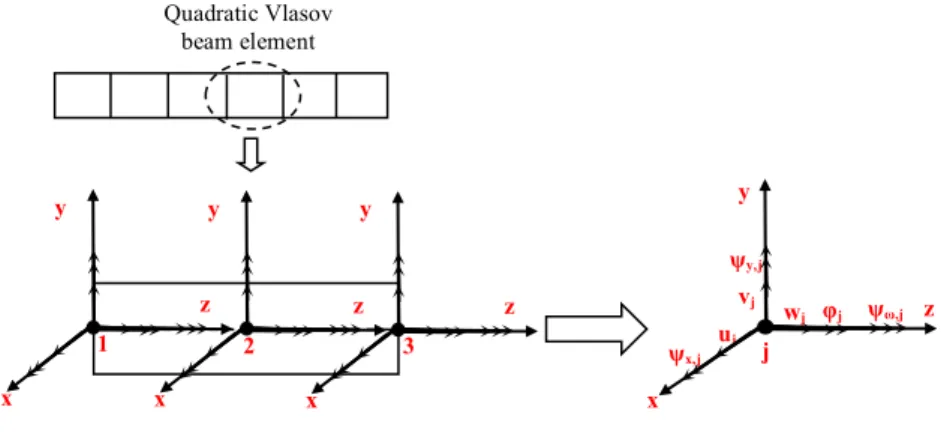
analysis have been extracted from the theories of Vlasov [1] and Gjelsvik [2]. Hodges et al [3] ap-plied the Variational Asymptotic Method (VAM) to non-linear three dimensional analysis of beams, obtaining the well-known VABS method (Variational Asymptotic Beam Section analysis), that reduces the three dimensional problem to a one-dimensional cross-sectional one, leading to the Vlasov beam element shown in the Figure 2 and used in this work.
In order to simplify the analysis of thin-walled beams, many authors have modeled the plate el-ements of the beams by separately using the CLPT theory [4,5], that can be done if transverse shear effects can be neglected. However, as it was shown by Gu and Chattopadhyay [6], the trans-verse shear strains have relevant effects in the case box beams made of anisotropic composite mate-rials, even for very thin-walled beams. In the present work, both transverse and warping shear strains are considered in the FEM formulation using the model proposed by Vo and Lee [7], but the warping shear strain energy is neglected in the shear correction factors computations based on the premise of small to moderate twist rotations.
Ones of the most valuable researches about the analytical and numerical treatment of the flex-ural-torsional behavior of thin-walled beams have been conducted by Jaehong Lee. A general theo-retical model based on the FSDT theory to describe the behavior of composites box beams under flexural and torsional loads was developed by this author and his co-workers, for both linear and non-linear problems [7,8]. The present work makes use of the aforementioned theoretical model, so it is concisely presented in the Part 2 of the paper. One substantial difference between the Lee’s model and the model presented here is the introduction of the shear correction factor into the varia-tional formulation for some special cases of laminates, as it is explained in Section 4. The shear-corrected linearized equation of motion in Updated Lagrangian formulation is presented in the Sec-tion 3.
As it was mentioned above, shear correction factors will be introduced into the variational for-mulation of the problem treated in this work for some special cases of plating. One of the most used methods for the shear correction factor determination comes from the theory of Mechanics of Lami-nated Beams (MLB) constructed by Barbero et al [9]. This theory has been employed by many authors to compute shear correction factors in analysis of pultruded composites beams [10,11] and it will be also used in this work to calculate the shear correction factors added in the stiffness matrix of the finite element model.
2 THE VLASOV WARPING THEORY AND THE MODEL OF LEE
Latin American Journal of Solids and Structures 10(2013) 647 – 673
In the Vlasov warping theory, for a free warping section, the axial displacement is compute by:
u! z =−ω s .ϕ!(z), where “z” represents the longitudinal axis of the beam and “s” is called the
contour coordinate of the section. For a restrained warping condition, normal stresses appear and
they can be expressed by: σ
!!,! s,z =−E z .ω s .ϕ!! z [14]. In the last expressions, ϕ is the twist
angle and ω(s) is called the warping function.
To a better understanding of the Vlasov warping theory, two coordinate systems are defined
(Figure 1): The Cartesian coordinate system (x,y,z), and the local plate coordinate system (n,s,z).
There is a point, P, with respect to which all global displacements and rotations are taken; this
point is called the pole, shear center or center of twists and the axis passing through it and parallel
to the “z” axis is called the pole axis; the angle of rotation of the cross section about that pole axis
is the twist angle (ϕ). Both coordinate systems are related between them by an angle θ.
Taking into account the Figure 1, the general expression for the warping function, ω(s), can be
written as [15]:
ω s = r s −F(s)
t(s) !
!!
.ds (1)
Figure 1 Coordinate systems of the Vlasov Warping Theory.
Where F(s) is the Saint-Venant circuit shear flow and t(s) is the thickness of each point of the
cross section. In the particular case of a box beams, the explicit expressions for the Saint-Venant
circuit shear flow, F(s), and the warping functions, ω(s), can be found in [16].
According to Vlasov theory, when the warping is restrained, a warping moment or bi-moment is originated in the cross-section. This moment is considered in the present work and its equation and relationship with primary Saint Venant torsional moment can be found in [14,17].
The present formulation is based on the one-dimensional Vlasov beam element [8,18-21], in which seven degrees of freedom are considered per master node (Figure 2), namely one axial
dis-P
x, u y, v A
n, u* s, v*
r
q
θ φ
z, w*
Latin American Journal of Solids and Structures 10(2013) 647 – 673
placement, two transverse displacements, one torsional rotation, two flexural rotations and one warping rotation. The last rotation is a measure of the warping intensity and its rate, of the magni-tude of the warping moment [22].
Figure 2 Vlasov beam element.
In the Vlasov beam element, transverse shear strains γ!" and γ!" and warping shear strain γ!
are included and it is assumed that they are uniform in each cross section of the beam element. According to this consideration and to the assumptions of the FSDT theory, Vo and Lee [7,8,23] obtained the following relationships (See Figure 1 for reference):
• Displacement field of the contour midline in terms of displacements of the pole point P:
u∗ s,z =u z .sen θ s −v z .cos θ s −ϕ z .q(s) (2a)
v∗ s,z =u z .cos θ s +v z .sen θ s +ϕ z .r(s) (2b)
w∗ s,z =w z +ψ! z .x s +ψ! z .y s +ψ! z .ω s (2c)
• Displacement field of any generic point C in the section in terms of displacements of the contour
midline (FSDT theory):
u! n,s,z =u∗(s,z) (3a)
v! n,s,z =v∗ s,z +n!ψ!∗(s,z) (3b)
w! n,s,z =w∗ s,z +n!ψ!∗(s,z) (3c)
Where“n!” is the distance along the normal direction between the midline contour and the
ge-neric point C and ψ!∗(s,z) and ψ!∗(s,z) denote the rotations of transverse plane about the “z”
and “s” axis of the local plate coordinate system, respectively. The expressions for those
rota-tions can be found in [7,8]. 1
x
z y
2
x
z y
3
x
z y
uj vj
wj ψy,j
ψx,j
ψω,j φj Quadratic Vlasov
beam element
j
x
Latin American Journal of Solids and Structures 10(2013) 647 – 673
3 ST R A IN S, ST R E SS R E SU LT A N T S A N D C O N ST IT U V E R E LA T IO N SH IP S
In the UL formulation, the work-conjugated pair used for the variational statement is the Almansi strain- Cauchy Stress tensor. In agreement with many authors that have analysed large deformation in Timoshenko`s beams [7,8,24,25], only nonlinear terms product of the variation in the longitudinal direction of transverse displacements will be considered in this work (Von Karman strains), leading
to the following simplification of the Almansi strain tensor for any generic C point on the contour:
e
!!,! n,s,z
!!∆! =! !!(!,!) !!∆! !!! − ! !. !!!∆!!! !!! ! + ! !! !!∆! !!! ! (4a) e!",! !!∆!
n,s,z =!
!
!!!∆!!!!,!
!!! +
!!!∆!!!(!,!)
!!! (4b)
e !",!
!!∆!
n,s,z = ! !!(!,!) !!∆!
!!! +
!!!∆!!!!,!
!!! (4c)
A more complex analysis of composites beams by FSDT considering the whole terms of the strain tensor can be found in [26], where the shear locking effects are reduced significantly, but the computational cost is high. In this case, for sake of numerical simplicity, shear locking is dealt with the application of a reduced integration scheme in the components of the linear stiffness matrix
containing A!!, A!" and A!!, which are shear extensional stiffnesses implicit in some coefficients of
the constitutive matrix of the composites box beam.
Following the same procedure employed by Machado and Cortínez [27], the following expressions
are gotten for the Von Karman strains of a generic C point in terms of the strains and curvatures of
the midsurface of the wall:
e
!!,! n,s,z
!!∆!
= e
!!,!(
!) s,
z + κ
!!,!(!) s,z .n!
!!∆! !!∆!
+κ
!!,!(!) s,z .n!! (5a)
e!",! n,s,z
!!∆!
= e!",!(!) s,z + 1 2 κ!",!(!) s,z .n!
!!∆! !!∆!
(5b)
e
!",! n,s,z
!!∆!
= e
!",!(
!) s,
z + 1 2 κ
!",!(!) s,z .n!
!!∆! !!∆! (5c) Where: e !!,!( !) !!!!
s,z , !!!!e!",!(!) s,z and e
!",!(
!)
!!!!
s,z are the Almansi strains in the midsurface
κ
!!,!(!) s,z
!!∆!
,!!∆!κ!",!(!) s,z and κ
!",!(!) s,z
!!∆!
are the biaxial curvatures in the midsurface.
κ
!!,!(!) s,z
!!∆!
is the high order biaxial curvature in midsurface of the wall.
Latin American Journal of Solids and Structures 10(2013) 647 – 673
Based on the constitutive in-plane and out-plane relationships for a lamina [28], direct constitu-tive equations relating the stress resultants and the global strains and curvatures of the cross sec-tion can be obtained, as it is detailed in [29]. In general, these expressions can be represented in UL formulation as:
F
! !!!!
=E.!!!!ε (6)
Where: !F
!!!!
= [N
!;M!;M!;M!;M!;V!;V!;T;R!]
! !!!!
,
ε !!!!
= ε
!;κ!;κ!;κ!;κ!";γ!";γ!";γ!;λ!
!!!!
The explicit values for E!" can be gotten from [8,29].
4 SHEAR CORRECTION FACTOR
Like in most of the works about thin-walled composite beams considering shear deformability
[7,22,30], here it is assumed that shear transverse strains (γ!",γ!") and warping shear strains (γ!)
are uniform over the entire cross sections of the beam. This assumption leads to uniform shear
strain energy in the global coordinate system (x,y,z), which is not necessarily true in most of cases.
To account for the error involved in this assumption, they are introduced shear correction factors into the constitutive relationships of shear stress and shear strains [28].
There are several methods to determine the shear correction factors in cross-section composites beams [31-36]. In this work, an energy-based method coming from the MLB theory of Barbero et al [9] is employed and it is briefly exposed in the next lines.
Considering small to moderate twist angles, the contribution of the warping shear strain energy to the average shear strain energy can be neglected according to [37], leading to the next expression for the average shear strain energy per unit length in a cross section of the beam (superscripts and subscripts indicating the configuration are suppressed for sake of simplicity):
u!"#$%=1
2
V
!γ!"+V!γ!" (7)
Latin American Journal of Solids and Structures 10(2013) 647 – 673
u!"#$=1
2 V!",!"#$
∗ γ!"! +V
!"∗ ,!"#$γ!"
! +
M∗!,!"#$κ!" !+R∗!,!"#$κ!" ! .ds!
!!,! !!,! ! !!! (8a) u !"#$%&'= 1
2 V!",!"#$%&'
∗ γ!"(!)+V
!"∗ ,!"#$%&'γ!"( !)+
M!∗,!"#$%&'κ!"(!)+R∗!,!"#$%&'κ!"(!) .ds! !!,!
!!,!
!
!!!
(8b)
The expressions for local laminate stress resultants appearing in equation (8) are:
V
!",∗ !=A!"ε!!,! (!) +
B!"κ!!,! (!) +
D!"κ!!,! (!) +
A!!γ!",! (!)+
B!!κ!",! (!):
Local laminate load in the contour direction
(9a)
V
!"∗ ,!=A!!γ!",!
(!)
+B!!κ !",! (!)
:
Local laminate load in the normal direction (9b)
M!∗,!=B!"ε!!,!
(!)
+D!"κ
!!,! (!)
+F!"κ
!!,! (!)
+B!!γ!",
! (!)
+D!!κ
!",! (!)
(9c)
R∗!,!= σ!"n.dn !!!!
!! !
! !"#$%
!!!
=B!!γ!",!
(!)
+D!!κ !",!
(!) (9d)
Where “i” represents both the flanges and the webs.
Now, considering thin-walled hollow beams, they are neglected the shear deformations in the
flanges and webs caused by the local laminate load in the normal direction, V
!"∗ ,!, [9] what is
equiva-lent to say that the shear stresses σ
!",! are not considered in this case for the computing of the shear correction factor. According to these assumptions, the equilibrium equations for any point in the cross section are:
∂σ!!,
!
∂s +
∂σ!", !
∂s =0 (10a)
∂σ!", !
∂z =0 (10b)
Latin American Journal of Solids and Structures 10(2013) 647 – 673 N
!∗=A!!ε!!+ A!!x s +B!!sin θ s κ!+ A!!y s −B!!cos θ s κ!
+ A!" γ!"cos θ(s) + γ!"sen θ(s) +A!".κ!" (11)
The equations (6) and (11) are used to obtain an explicit expression for N
!∗ in terms of the
re-sultants N
!, M!, M!, M!, V! and V! (bimoment, secondary torsional moment and high order normal
force are not considered). The shear flow variation in the “i" wall is then obtained by using equation
(10a) and from the equilibrium equations for a beam subjected to flexion and Saint Venant torsion. The final expressions are:
• For the flanges:
V
!",!,∗ !"#$%&'= A!",!"#$%&'+B!",!"#$%&'.x(s) V!+ A!",!"#$%&'+B!",!"#$%&'.x(s) w! (12a)
• For the webs:
V
!",!,∗ !"#$= A!",!"#$+B!",!"#$.y(s) V!+ A!",!"#$+B!",!"#$.y(s) w! (12b)
Where “w
!(z)” and “w!(z)” are the distributed loads and “e!” and “e!” are the eccentricities of
those loads.
The explicit expressions for the constants of the equations (12a) and (12b) can be found in
Ap-pendix A, where “α” is the shear-corrected constitutive matrix (See equation 16).
The integration of equations (12a) and (12b) to obtain expressions for the shear flow in the flanges and webs is done as it is described in [39] for closed sections.
According to [28], the shear-extension and bending-twisting coupling can be suppressed for lami-nates with off-axis plies balanced symmetrically (antisymmetric angle-ply laminate, for example). If
the laminate is symmetric, not necessarily balanced, the coupling matrix, B, is equal to zero. In this
work, only the former case will be considered for the shear correction factor calculations; the second case will be considered in further works. So, neglecting high order biaxial curvatures and consider-ing all assumptions mentioned so far, the constitutive relationships of equations (9) are reduced to:
V
!",∗ !=B!"κ!!,! (!)
+A!!γ!",
! (!)
(13a)
M!∗,!=B!"ε!!,!
(!)
+D!!κ
!",! (!)
(13b)
As the layers of the laminate are thin enough, the influence of the coupling term B!" is small
enough too, and in this case, the biaxial curvature κ
!" (!)
=−2∂!u ∂s∂z is neglected for the
Latin American Journal of Solids and Structures 10(2013) 647 – 673
u!"#$=!
!
!!"∗,!"#$!
!!!,! . ds ! !!, ! !!,! !
!!! (14a)
u
!"#$%&'=
!
!
!!"∗ ,!"#$%&' !
!!!,! . ds ! !!,! !!,! !
!!! (14b)
The shear correction factors are introduced into the constitutive relationships for V
! and V!, as it
is indicated in the next equations (sum convention):
V
!=K!"E!"ε! (15a)
V
! =K!"E!"ε! (15b)
The last equations lead to a modified constitutive matrix, α, defined as:
α= E!",E!",E!",E!",E!",K!"E!",K!"E!",E!",E!" (16)
The final expressions to find the shear correction factors are gotten by equating the average shear strain energy to the actual shear strain energy:
Equation for Ksx:
!!"∗ ,!"#$%&' !
!!!,! .ds!
!!,!
!!,!
!
!!! =
V
!",∗ !"#$%&' .ds! !!,
! !!,!
!
!!! α!"!!N!+α!!"!M!+α!"!!M!+
α
!"
!!M
!+α!!!! V!",∗ !"#$%&' .ds!
!!,!
!!,!
!
!!! +α!"!! V!",∗ !"#$ .ds! !!,! !!,! ! !!! (17a)
Equation for Ksy:
!!"∗ ,!"#$!
!!!,! . ds ! ! !,! !!,! ! !!! = V
!",∗ !"#$ .ds! !!,!
!!,!
!
!!! α!"!!N!+α!!"!M!+α!"!!M!+
α!"!!M!+α!"!! V
!",∗ !"#$%&' .ds! !
!,! !!,!
!
!!! +α!!!! V!",∗ !"#$ .ds!
Latin American Journal of Solids and Structures 10(2013) 647 – 673
In linear analysis, the resultants appearing in Equations (17) are known in advance from the equi-librium equations in each section. In non-linear analysis, they are taking the resultants from the last configuration.
In the numerical examples presented here, they are reported the averaged values of the shear correction factors computed for the cross sections of the beam considered in the finite element anal-ysis.
5 FINITE ELEMENT FORMULATION
This analysis is limited to box beams with equal-thickness flanges and equal-thickness webs, in such
a way that the pole point coordinate (�
!,�!) is located in the centroid of the beam. The basic steps
of the continuum mechanics incremental decomposition for UL formulation as stated in [4] are ap-plied to this analysis and it is obtained the following linearized equation of motion, where the shear correction factor as calculated on the Section 4 is introduced into the constitutive relationships of
the shear stress resultants, �!and �
!.
ℛ !!!!
−1 2 �
! !
.� �
!,!
! + �!"
!!!!
.� �!",
!
! + �!"
!
.� �!",
!
!
! !
� !�
= �!!�!+�!"�!!+�!"�!!+�!"�!! +�!" �!−�! +�!" �!+�!
! !
!
+�!" �!+�! +�!" �!+�! .� !�!
+ �
!"�!+�!!�!! +�!"�!!+�!"�!! +�!" �!−�! +�!" �!+�!
+�!" �!+�! +�!" �!+�! .� !�!!
+ �!"�!+�!"�!! +�!!�!!+�!"�!! +�!" �!−�! +�!" �!+�!
+�!" �!+�! +�!" �!+�! .� !�!!
+ �
!"�!+�!"�!! +�!"�!!+�!!�!! +�!" �!−�! +�!" �!+�! +�!" �!+�! +�!" �!+�! .� �!!
!
+��� �!"�!+�!"�!! +�!"�!!+�!"�!! +�!" �!−�! +�!! �!+�!
+�!" �!+�! +�!" �!+�! � !�!+ !�!
+��� �!"�!+�!"�!!+�!"�!! +�!"�!! +�!" �!−�! +�!" �!+�!
+�!! �!+�! +�!" �!+�! � !�!+ !�!
+ �!"�!+�!"�!! +�!"�!!+�!"�!! +�!" �!−�! +�!" �!+�!
+�!" �!+�! +�!! �!+�! � !�!+ !�!
+ �!"�!+�!"�!! +�!"�!!+�!"�!! +�!! �!−�! +�!" �!+�!
+�!" �!+�! +�!" �!+�! � !�!− !�! � !�
Latin American Journal of Solids and Structures 10(2013) 647 – 673
From last equation, explicit expressions for the linear stiffness matrix can be stated. The non-linear stiffness matrix components are established in terms of the resultant loads in the current configura-tion.
Considering only the transverse loads and the torsional moments, the vector of external forces for an element has the next form:
f = 0;0;f!;f!;0;0;0 (19)
For the distributed loads, q (distributed transverse load) and t (distributed torsional moment),
the load assigned to each node, “i", is defined as: f!(i)= q(ξ).φ! ξ .J ξ .dξ
!
!! and
f!(i)= t(ξ).φ! ξ .J ξ .dξ !
!! .
For punctual loads, Q (punctual transverse load) and T (punctual torsional load), the load
as-signed to each node, “i", is defined as: f! i =φ! ξ! .Q and f! i =φ! ξ! .T , where ξ! is the point
of application of the punctual loads, Qand T, in the isoparametric coordinate system.
The final non-linear finite element formulation is represented by:
R(!!∆! ∆ )
!!∆!
=T ! ∆ . ! δ∆ (20)
Where:
R(!!∆! ∆ )
!!∆!
=!!∆! F −!!∆! K!(!!∆! ∆ ) .!!∆! ∆ :
Residual matrix at configuration “t+Δt” (21a)
T ! ∆ = K! ∆
! !
+ ! K!" ! ∆ :
Tangent stiffness matrix (21b)
δ∆ ! :
Incremental matrix (21c)
The Newton-Raphson method is used to solve the equation (20) [41]. In this method, both
tan-gent stiffness matrix, T ! ∆ , and the residual vector, !!∆! R(!!∆! ∆ ) , are updated during each
Latin American Journal of Solids and Structures 10(2013) 647 – 673
6 RESULTS AND DISCUSSIONS
6.1 Result comparison with analytical models
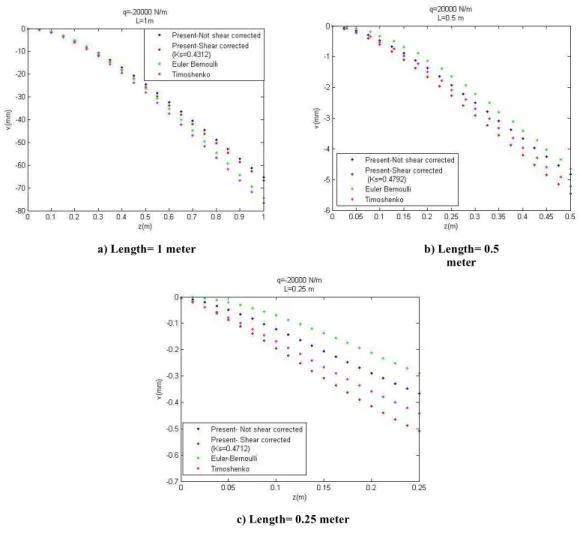
Both Euler-Bernoulli and Timoshenko beam models are used to estimate the vertical displacements in several locations of a cantilever composite box beams supporting a central distributed load. The whole sides of the box beam have the same laminate, which is done of chopped strand mats of E
fiberglass with vinylester resin, having the following mechanical properties
[42]:E!=E!=14236 MPa, ν!"=0.3287 and G!"=G!"=G!"=5357 MPa. Some comparisons
be-tween these analytical models and the present numerical model are shown in Figure 4. As it can be appreciated, the present numerical solution is closer to the analytical solution of Timoshenko when the beam is shorter, and this matching is improved by the introduction of the shear correction
fac-tor, K!", into the variational formulation. Despite the introduction of a reduced integration scheme
into some terms of the stiffness matrix, the shear locking is yet appreciated, principally when beam is large, where stiffening effects in the results are more notorious. In this particular problem, the
shear correction factor is K!",!"#$#%&=0.4712 for L=0.25 m; the difference with the one computed
by Bank [33] is 12.27 % (K!",!"#$=0.4197) and 8.50% is the difference with the factor calculated
by Cowper [32] (K!",!"#$%&=0.4355).
Figure 4 Comparison between analytical models and the actual numerical model for different lengths of beam. a) Length= 1 meter b) Length= 0.5
meter
Latin American Journal of Solids and Structures 10(2013) 647 – 673 6.2 Results comparison with other models for nonlinear analysis of composites box beam
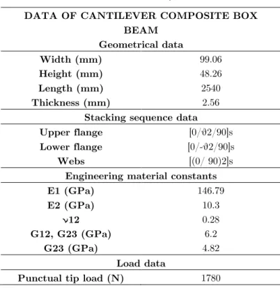
A non-linear problem proposed in [7] and [43] will be considered for comparison purposes. The prob-lem consists in a cantilever composite box beam with the next data (see Table 1)
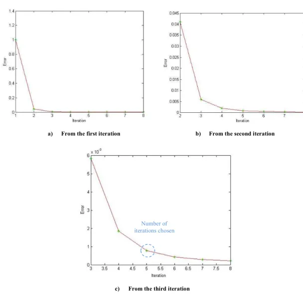
The updated Lagrangian finite element model exposed in Section 5 is used, but the shear correc-tion factor calculated as proposed here cannot be used in this example because the off-axis plies in the stacking sequence are not balanced. The number of iterations for each load step is determined
in function of a minimum allowable value of E(δΔ)=10!!, as it is showed in Figure 5, where the
error is plotted as function of the iterations to obtain the equilibrium configuration, considering
θ=45° in the flanges. It can appreciate that this particular problem is very stable, because the
increase in the number of iteration leads to a reduction in the error, which is not ever the case.
Table 1 Data of cantilever composite box beam
DATA OF CANTILEVER COMPOSITE BOX BEAM
Geometrical data
Width (mm) 99.06 Height (mm) 48.26 Length (mm) 2540 Thickness (mm) 2.56
Stacking sequence data Upper flange [0/θ2/90]s
Lower flange [0/-θ2/90]s
Webs [(0/ 90)2]s Engineering material constants E1 (GPa) 146.79 E2 (GPa) 10.3
ν12 0.28
G12, G23 (GPa) 6.2 G23 (GPa) 4.82
Load data
Latin American Journal of Solids and Structures 10(2013) 647 – 673
Figure 5 Change of the error with the number of iterations for a determined load step.
For θ=45°and θ=90°, the results obtained from various authors for the vertical displacement,
“v”, the horizontal displacement, “u”, and the twist angle, "∅", in the tip of the cantilever beam, are
showed in Table 2.
Number of iterations chosen
a) From the first iteration b) From the second iteration
Latin American Journal of Solids and Structures 10(2013) 647 – 673 Table 2 Vertical displacement for the cantilever composite box beam problem being considered
Vertical displacement, v.
Reference θ=45° θ=90° Stemple and Lee [44] 48.50 cm 53.40 cm Vo and Lee (FSDT) [7] 55.00 cm 56.5 cm Vo and Lee (CLPT) [43] 51.3 cm 52.9 cm
Present 58.8 cm 59.12 cm
Horizontal displacement, u.
Reference θ=45° θ=90° Stemple and Lee [44] 1.35 cm 0.06 cm Vo and Lee (FSDT) [7] 1.20 cm 0.03 cm Vo and Lee (CLPT) [43] 1.00 cm 0.01 cm
Present 0.91 cm 0.03 cm
Twist angle, ∅.
Reference θ=45° θ=90° Stemple and Lee [44] 0.09 rad’s 0 rad’s Vo and Lee (FSDT) [7] 0.072 rad’s 0 rad’s Vo and Lee (CLPT) [43] 0.065 rad’s 0 rad’s Present 0.045 rad’s 0 rad’s
The Table 2 indicates that the present formulation predicts larger vertical displacements of the box beam than other well-known models developed up to now. As in the models developed by Vo and Lee [7,43], this UL model predicts very closed values of the vertical displacement of the tip of
the beam for stacking sequences in the flange with θ=45° and θ=90°, from which it can be
in-ferred a weak influence of the angle θ in the vertical displacement of the beam in this range, what
can be confirmed in the mentioned works [7, 43]. Contrary to the vertical displacement, the present UL model is stiffer than the other ones considered here for the horizontal displacement and the twist angle.
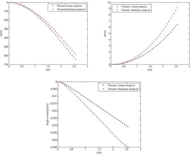
In Figure 6, it is showed the change of the three degrees of freedom considered in this example
(v,u,ϕ) in the longitudinal direction of the beam for θ=45°, solving the problem linearly and
Latin American Journal of Solids and Structures 10(2013) 647 – 673
Figure 6 Differences between linear and UL non-linear solutions for v,u and ∅.
6.3 Result comparison with experimental data
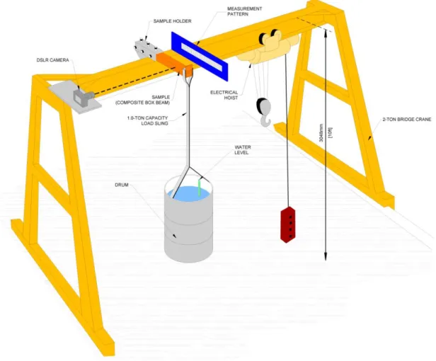
For verification purposes, a cantilever short composite box beam was subjected to several loads in the tip. The whole experimental setup, which allows both applying instantaneous load and measur-ing directly the respective deflection, is shown in Figure 7. The setup consists of a 2-ton bridge crane, a sample holder, an electrical hoist, a 1-ton capacity load sling and an open drum with lifting accessories. The upper part of setup also includes a DSLR camera at the same level of the compo-site box beam behind which is installed a measurement pattern to record (by a picture) the deflec-tion at the moment when each load is applied.
Latin American Journal of Solids and Structures 10(2013) 647 – 673
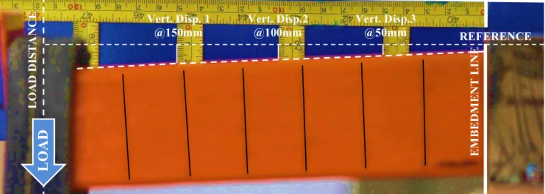
measurement stations and the vertical ones installed each 2 inches, to measure the vertical dis-placement directly when the picture was taken.
Several punctual loads were applied at the tip of the box beam with the objective to evaluate the vertical displacements at determined locations. The first step was calculating the drum´s tare and takes it into account in the mass. Then, at the floor level without the load sling connected to the drum, the recipient was filled until a predetermined level, taking care to measure exactly the quantity of liquid added; this mass of water plus the drum’s tare and load sling´s weight are summed to calculate the first load that was applied to the tip of the beam. The mass was elevated using the electric hoist, then the load sling was connected to the drum and the load was applied obtaining a specific vertical displacement.
After the vertical displacement is measured digitally in the picture, the box beam is completely unloaded using the electric hoist. More water is added and the load process in the box beam is repeated several times, like it was explained above.
Latin American Journal of Solids and Structures 10(2013) 647 – 673
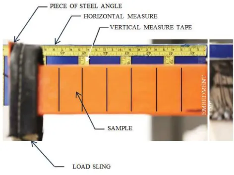
Figure 8 Sample installation details.
The properties of the material of the box beam were obtained from manufacturer’s information and they are exposed in Table 3.
Table 3 Specifications of the composites box beam.
Geometrical specifications Width (mm) 50.8 Height (mm) 50.8 Thickness (mm) 4.08
Stacking sequence Flanges and webs [0]6
Material properties E1 (GPa) 6.8 E2 (GPa) 1.61 G12, G13 (GPa) 2.72 G23 (GPa) 1.89
ν12 0.15
In the Figure 10, they are plotted the vertical displacements of the short beam obtained from
the present model, considering the not shear and shear corrected (K!"=0.415) variational
Latin American Journal of Solids and Structures 10(2013) 647 – 673
the approximation of measurements and the lack of parallelism in the camera (despite special care-ful was taken in the visual alignment, no parallelism verification devices at milimetric scale were employed) and errors in the characterization of the properties of the material coming from the manufacturer. The average relative errors point to conclude that the addition of the shear correc-tion factor into the variacorrec-tional formulacorrec-tion originates numerical solucorrec-tions better approximate to experimental data for the case of linear analysis, which is the one considered in this section.
Figure 10 Vertical displacements of the box beam using the not shear and shear corrected present model.
EM
BED
M
EN
T
LI
N
E
REFERENCE LINE Vert. Disp. 1
@150mm
Vert. Disp.2 @100mm
LO
A
D
D
IS
TA
N
C
E Vert. Disp.3
@50mm
Figure 9 Box-Beam behavior due to 2141N. Distances and deflections
LO
A
Latin American Journal of Solids and Structures 10(2013) 647 – 673
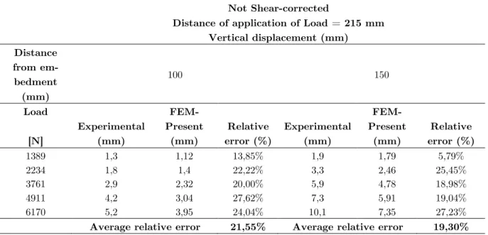
Table 3 Comparison between numerical results an experimental data for the not shear corrected model.
Not Shear-corrected
Distance of application of Load = 215 mm Vertical displacement (mm) Distance
from em-bedment
(mm)
100 150
Load Experimental (mm) FEM-Present (mm) Relative error (%) Experimental (mm) FEM-Present (mm) Relative error (%) [N]
1389 1,3 1,12 13,85% 1,9 1,79 5,79%
2234 1,8 1,4 22,22% 3,3 2,46 25,45%
3761 2,9 2,32 20,00% 5,9 4,78 18,98%
4911 4,2 3,04 27,62% 7,3 5,91 19,04%
6170 5,2 3,95 24,04% 10,1 7,35 27,23%
Average relative error 21,55% Average relative error 19,30%
Table 4 Comparison between numerical results an experimental data for the shear corrected model.
Shear-corrected
Distance of application of Load = 215 mm Vertical displacement (mm) Distance
from em-bedment
(mm)
100 150
Load Experi-mental (mm) FEM-Present (mm) Relative error (%) Experi-mental (mm) FEM-Present (mm) Relative error (%) [N]
1389 1,3 1,15 11,54% 1,9 1,82 4,21%
2234 1,8 1,53 15,00% 3,3 2,82 14,55%
3761 2,9 2,61 10,00% 5,9 5,02 14,92%
4911 4,2 3,42 18,57% 7,3 6,24 14,52%
6170 5,2 4,4 15,38% 10,1 8,03 20,50%
Average relative error 14,10 % Average relative error 13,74%
6.4 Case study
The geometry, boundary conditions and lamina material of the composite box beam employed in Section 5.2 will be used in this case study and they are taken into account the following stacking
sequences for both flanges and webs: [(θ/-θ)2]s (balanced and symmetrical), [(θ/-θ)4] (balanced and
Latin American Journal of Solids and Structures 10(2013) 647 – 673
are analyzed as function of the orientation of the fibers and it is also examine the influence of the shear correction factor in the angle of twist.
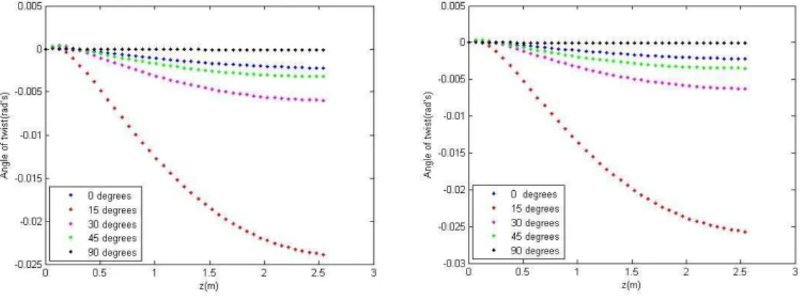
In Figure 11, it is showed the variation of the twist angle for several values of the angle θ,
con-sidering a distributed load of q=−1000 N/m. As it can be seen, for most of fiber orientations, θ, a
torsional coupling appears for the balanced and symmetrical laminate and the angles of twist pre-dicted can be initially attributed to geometric nonlinearities and to the twisting-flexural coupling,
D!". In the case of the angle-ply antisymmetrical laminate, the results obtained are only slightly
larger than the ones of the balanced and symmetrical plating. This means that in this particular case study, the material coupling terms D16 (present in the balanced and symmetrical laminate) and B16 (present in the angle-ply antisymmetrical laminate), have not a strong influence at
induc-ing twist angles; therefore, in the first two stackinduc-ing sequence analyzed, [(θ/-θ)2]sand [(θ/-θ)4], these
twist angles can be essentially attributed to a bending-twisting coupling coming from the high order
coupling terms, F!", originated from geometric nonlinearities [8,29]. The most important coupling
torsion effects can be seen when plies are oriented in the ±15° directions, which is consistent with results of [7]. For the symmetrical non-balanced stacking sequence considered in this case study, a stronger twisting- flexural and shear-extensional coupling can be observed, if the results are com-pared with the former two cases mentioned, being the maximum values of twist angles reached again in the ±15° directions, corroborating again the results of [7]. In this case, all terms of coupling
matrix, B, are zero, but the shear-extensional (A16) and twisting-flexural (D!") coupling terms still
remains, and when compare Figure 11c with Figures 11a and 11b, it can be appreciated that the non-balancing of off-axis plies in the laminate brings to a significant influence of those material coupling terms in the twist angle.
In Figure 11, it can be observed that the change of the angle of twist is not constant for some
fiber θ orientations. It is an indication of the presence of variable warping effects, and this can be
confirmed in the Figure 12, where the variation of the angle of warping in the longitudinal direction
of the beam is plotted, for the unbalanced symmetrical plating [0/θ2/0]s. For θ=0°and θ=90°,
no significant warping angles are predicted by the model, what is consistent with the small values of the twist angles predicted in those fiber orientations. However, for other fiber orientations, warping angles are important. The longitudinal location of the point supporting the maximum warping ef-fects is variable with the angle of orientation of fibers and the most relevant warping efef-fects are
presented when fibers are oriented at θ=15°. From the point of view of the induced warping
ef-fects, the behavior of the plot indicates that the most critical section for the cantilever beam is among the fixed support, where warping moment is the maximum, and approximately 0.55 meters from that support, where warping deformation is the highest.
In order to examine the influence of the shear correction factor, K!", into the results of the
pre-sent UL formulation, the twist angles computed for the beam not shear and shear-corrected are plotted in Figure 13 for the balanced non-symmetrical stacking sequences considered in this case
study, [(θ/-θ)4]. In this figure, it is clearly appreciated that the introduction of K
!" into the
non-
Latin American Journal of Solids and Structures 10(2013) 647 – 673
linear analysis. This can be explained studying the assumptions implicit in the shear correction factors calculations. The material decoupling assumptions are related to the off-axis balanced sym-metrically stacking sequence and to the small thickness of each lamina of the laminate, what is complied in this particular case. Another important assumption is the non-consideration of the shear stresses in the normal direction of the local plate coordinate system; this assumption is valid for walls with small thickness, what is complied in this case too. The other important assumption is to neglect the warping and high order shear strain energies; the small contributions of these energies to the total shear strain energy cannot be guaranteed in this case and the error associated to that assumption is probably the main cause of the instability of the shear-corrected solution for the twist angles, what suggests that those shear strain energies shall be considered in the shear correction factor computation for this kind of non-linear problems.
Figure 11 Variation of angle of twist in the longitudinal direction for several stacking sequences. a) Balanced and symmetrical, [(θ/-θ)2]s b) Balanced and non-symmetrical, [(θ/-θ)4]
Latin American Journal of Solids and Structures 10(2013) 647 – 673 Figure 12 Angles of warping for several longitudinal location of the box beam
Figure 13 Influence of the shear correction factor, Ksy, in the twist angle predictions by the UL model for non-linear analysis.
7 CONCLUDING REMARKS AND FUTURE WORKS
Latin American Journal of Solids and Structures 10(2013) 647 – 673
order shear strain energies into the calculation of the shear correction factors; these strain energies can have an important contribution in some problems of composites box beams undergoing large displacements according to the results obtained in the present work.
Future works will be focused on the development of shear-corrected UL finite element models to predict large twist rotations, where the model for the calculation of the shear correction factors incorporated into the variational formulation, accounts for the warping and high order shear strain energies.
Acknowledgement The authors of this work are grateful to Centro de Investigación of Instituto Tecnológico Metropolitano at Medellín, Colombia for the financial support for the development of the present research.
References
[1] Vlasov V.Z. Thin-walled elastic beams. 2nd edition. Jerusalem (Israel). Israel Program for Sci-entific tranlastion. 1961.
[2] Gjelsvik A. The theory of thin walled bars. New York. John Wiley and Sons Inc. 1981.
[3] Hodges D.H., Altigan A.R., Cesnik C.E., Fulton M.V. On a simplified strain energy function for geometrically non-linear behavior of anisotropic beams. Composites Engineering 1992; 2(5-7):513-526.
[4] Kosmatka J.B., Friedman P.P. Vibration analysis of composites turbopropellers using a non-linear beam type finite element approach. AIAA J., 1989, 27(11) 1606-1614.
[5] Rehfield L.W., Altigan A.R., Hodges D.H. Nonclassicalbehavior of thin-walled composite beams with closed cross sections. Journal of American Helicopter Society. 1990, 35, 42-50.
[6] Gu H., Chattopadhyay A. A new higher order plate theory in modeling delamination buckling of composites laminates.AIAA J. 1994, 32(8), 1709-1716.
[7] Vo T.P. Lee J. Geometrically non-linear theory of thin-walled composites box beams using shear deformable theory. International Journal of Mechanics Science 52 (2010) 65-74.
[8] Vo T.P., Lee J. Flexural-torsional behavior of thin-walled composite box beams using shear-deformable beam theory. Engineering Structures 30 (2008) 1958-1968.
[9] Barbero E. Lopez-Anido J.R. (1993). On the mechanics of thin-walled laminated composite beams. Journal of Composite Materials 27(8): 806-29.
[10] Davalos J.F. et al. Analysis and design of pultruded FRP shapes. Composites: Part B 27B (1996) 295-305
[11] Hayes M.D. Lesko J.J. The Effect of Non-Classical Behaviors on the Measurement of the Ti-moshenko Shear Stiffness.Proceedings of the 2nd International Conference on FRP Composites in Civil Engineering - CICE 2004, 8-10 December 2004, Adelaide, Australia
[12] Haukaas T. The Vlasov Warping theory. Lecture Notes. University of British Columbia. 2002.
Latin American Journal of Solids and Structures 10(2013) 647 – 673
[14] Ringsberg J. Vlasov torsion theory. Chalmer University of Technology.Lecture Notes. 2000.
[15] Krenk S. y Gunneskov O., Statics of thin walled pretwisted beams, International Journal of Numerical Methods in Engineering, 17, 1981 pp.1407-1426.
[16] Phuong T., Lee J. Flexural-torsional behavior of thin-walled closed-section composite box beams. Engineering Structures 29 (2007) 1774-1782.
[17] Bombassaro E. Preliminaries in warping torsion. Lecture Notes. Graduiertenkolleg 1462 Bau-haus-UniversitatWeimar.Dezember 2009.
[18] Dvorkin E. et al. A Vlasov beam element.Computers and Structures.Vol 33.No.1, pp.187-196, 1989.
[19] Mottershead. J.E.. Warping torsion in thin-walled open section beams using the semiloof beam element.International Journal of Numerical Methods in Engineering (26) 231-243 (1988).
[20] Phuong T., Lee J. Flexural-torsional behavior of thin-walled closed-section composite box beams. Engineering Structures 29 (2007) 1774-1782.
[21] S.W. Lee and Y.H. Kim. A new approach to the finite element modeling of beams with warp-ing effect. International Journal of Numerical Methods in Engineerwarp-ing (24) 2327-2341 (1987)
[22] Cortínez V. Rossi R.E. Vibrations of pretwisted thin-walled beams with allowance for shear deformability. COMPUTATIONAL MECHANICS. New Trends and Applications. CIMNE, Barcelona, Spain 1998.
[23] Lee J. Flexural analysis of thin-walled composite beams using shear-deformable beam theory. Composites Structures 70 (2005) 212-222.
[24] Menzala G.P. Zuazua E. The beam element equation as a limit of a 1-d nonlinear Von Karman model.Applied Mathematics Letters.1999; 12: 47-52.
[25] Sciuva M.D. Icardi U. Large deflection of adaptative multilayered Timoshenko beams.Composites Structures.1995; 31:49-60.
[26] Agarwal S. Chakraborty A. Gopalakrishnan S. Large deformation analysis for anisotropic and inhomogeneous beams using exact linear static solutions. Composites Structures 72 (2006) 91-104.
[27] Machado S. Cortínez V. Lateral buckling of thin-walled composite bisymmetric beams with prebuckling and shear deformation. Engineering Structures 27 (2005) 1185-1196
[28] Reddy J.N. Mechanics of laminated composite plates and shells: Theory and analysis. Second Edition.CRC Press. 2004.
[29] Librescu L., Song O. Thin-walled composite beams. Springer; 2006.
Latin American Journal of Solids and Structures 10(2013) 647 – 673
[31] Renton J.D. Generalized Beam Theory Applied to Shear Stiffness, International. Journal of Solids Structures, 27-15, 1955-1967, (1991).
[32] Cowper G.R. The Shear Coefficient in Timoshenko's Beam Theory, ASME, Journal of Applied Mechanics, 33, 335-340, (1966).
[33] Bank, L.C., Shear coefficients for thin-walled composite beams. Composite Structures, 1987.8(1): p. 47-61.
[34] Dharmarajan, S. and H. McCutchen, Shear Coefficients for Orthotropic Beams. Journal of Composite Materials, 1973.7: p. 530-535.
[35] Teh, K.K. and C.C. Huang, Shear Deformation Coefficient for Generally Orthotropic Beam. Fiber Science and Technology, 1979.12: p. 73-80.
[36] Stephen N.G. On Shear Coefficients for Timoshenko Beam Theory, Trans ASME, Journal of Applied Mechanics, 68, 959-960, (2001).
[37] Yoi C., Lee. S. Stability of Structures: Principles and applications. Chapter 6: Torsional and flexural-torsional buckling. Butterworth-Heinemann Elsevier. Oxford, UK. 2011.
[38] Chandra R., Stemple A.D., Chopra I. Thin-walled composite beams under bending, torsional and extensional loads. Journal of Aircraft. 1990; 27(7): 619-636.
[39] Megson T.H.G. Structural and stress analysis. Chapter 10 and 11. Butterworth Heinemann. 2nd Edition. 2000.
[40] Bathe K.J. Finite element procedures. Prentice Hall. 1996.
[41] Crisfield, M. A. Nonlinear finite element analysis of solids and structures. FirstEdition. Wiley&Sons. 1997.
[42] Miravete, Antonio. Materiales Compuestos I. 1ra Edición. INO Reproducciones S.A. Zaragoza, 2000.
[43] Vo T.P. Lee J. Geometrically nonlinear analysis of thin walled composite box beams. Comput-ers and Structures 87 (2009) 236-245
Latin American Journal of Solids and Structures 10(2013) 647 – 673 Appendix
Explicit expressions for the constants for shear flow calculation in webs and flanges.
Constants for flanges.
A!",!"#$%&'=−A!! α!"!!+
c !
2
α
!!!! −A!" α!"!!+α!"!! +B!!α!!!!
B!",!"#$%&'=−A!!α!"!!
A!",!"#$%&'=A!! α!!"!e!+α!"!!+
c !
2α!"!!e!+ c
!
2α!"!! +A!" α!"!!e!+α!!!!+α!!!!e!+α!"!! −B!! α
!" !!e
!+α!"!!
B!",!"#$%&'=A!! α!!"!e!+α!"!!
Constants for webs.
A!",!"#$=−A!! α!"!!+
c
!
2α!!
!! −A
!" α!"!!+α!"!! +B!!α!!!!
B!",!"#$=−A!!α!"!!
A!",!"#$=A!! α!"!!e!+α!"!!+
c
!
2α!"!!e!+ c
!
2α!"!! +A!" α!"!!e!+α!!!!+α!!!!e!+α!"!! −B!! α
!"
!!e !+α!"!!