Dynamic instability of laminated sandwich plates having inter-laminar imperfections with in-plane partial edge load-ing is studied for the first time usload-ing an efficient finite el-ement plate model. The plate model is based on a refined higher order shear deformation plate theory, where the trans-verse shear stresses are continuous at the layer interfaces with stress free conditions at plate top and bottom surfaces. A lin-ear spring-layer model is used to model the inter-laminar im-perfection by considering in-plane displacement jumps at the interfaces. Interestingly the plate model having all these re-fined features requires unknowns at the reference plane only. However, this theory requiresC1continuity of transverse dis-placement (w) i.e.,wand its derivatives should be continuous at the common edges between two elements, which is diffi-cult to satisfy arbitrarily in any existing finite element. To deal with this, a new triangular element developed by the authors is used in the present paper.
Keywords
dynamic instability, imperfection, partial edge loading, sand-wich plate, refined plate theory, Finite Element.
Abdul Hamid Sheikhb
a
Department of Civil Engineering, Indian In-stitute of Technology, Roorkee-247667, Ph. +91(1332)285844, Fax. +91(1332)275568 – India
b
School of Civil, Environment and Mining En-gineering (Office: EM111), University of Ade-laide, North Terrace, AdeAde-laide, SA 5005 – Aus-tralia
Received 22 Jun 2010; In revised form 22 Oct 2010
∗Author email: [email protected]
1 INTRODUCTION
The loads acting on parts of turbines, electric machines and parts of aircraft or ships due to aerodynamic and hydrodynamic effects are some typical examples of in-plane partial edge loads, which may induce dynamic instability. Dynamic instability of laminated sandwich plate sub-jected to in-plane partial edge loading is of considerable importance in mechanical, aerospace and many other engineering fields. The most important feature of laminated composite plates is that they are weak in shear compared to that of extensional rigidity. Due to this, the effect of shear deformation becomes very significant consideration for the analysis of such laminated structures. Moreover, the problem becomes much more complex if some inter-laminar im-perfection is found in the form of weak bonding or otherwise. All these aspects have been discussed in detail in some earlier paper by the authors i.e., Chakrabarti and Sheikh [2].
structure under in-plane loads over a range of excitation frequencies. The well-known Hill’s method of infinite determinants is used for solving a system of Mathieu-type equation in the present problem to predict the stability properties. Dynamic instability of plates under differ-ent in-plane loads has been investigated by a number of differdiffer-ent investigators in case of perfect interface. The dynamic stability of rectangular isotropic plates under various in-plane forces has been studied by Bolotin [1], Jagdish [10] and Yamaki and Nagai [16]. Hutt and Salam [9] and Deolasi and Datta [7] used finite element method based on first order shear deformation theory (FSDT) to study the parametric instability characteristics of thin isotropic plates. The dynamic stability of rectangular laminated composite plate due to periodic in-plane load is studied by Srinivasan and Chellapandi [14] using finite strip method (FSDT). Dynamic stabil-ity of laminated composite plates due to periodic in-plane loads is investigated by Chen and Yang [5] using FSDT. Dynamic instability of composite laminates has been studied by Kwon [11] (finite element method) and Chattopadhay and Radu [4] (analytical method) using Higher order shear deformation theory (HSDT). Lee [12] studied the finite element dynamic stability of laminated composite skew plates containing cutouts based on HSDT. Dynamic instability analysis of composite laminated thin walled structures has been carried out by Fazilati and Ovesy [8] by using two versions of FSM. Patel et al. [13] have done the parametric study on dynamic instability behavior of laminated composite stiffened plate by using the FSDT. Dynamic instability behavior of composite and sandwich laminates with interfacial slips has been studied by Chakrabarti and Sheikh [3] by using RHSDT (refined higher order shear deformation theory).
However, no studies based on RHSDT are found in the literature in case of imperfect laminated sandwich plates having in-plane partial edge loading. In this paper attempt has been made for the first time to study the dynamic instability of imperfect laminated sandwich plates with in-plane partial edge load using a finite element plate model recently developed by the authors based on RHSDT in combination with linear spring layer model. The problem is solved by finite element technique in order to have generality in the analysis and also to generate new results.
2 FORMULATION
Following the concept of refined higher order plate theory (RHSDT) and linear spring layer model discussed earlier, the through thickness variation of in-plane displacements (Fig. 1) may be expressed as follows.
¯
u=u+
nl
∑ i=1
{αix(z−zi+1)−∆ui}H(−z+zi+1)+
+
nl+nu
∑ i=nl+1
{αix(z−zi)+∆ui}H(z−zi)+βxz 2
+ηxz 3
Figure 1 General lamination lay up and displacement configuration.
The transverse displacement is assumed to be constant over the plate thickness i.e.,
¯
w=w. (3)
The stress-strain relationship of a lamina (sayk-th lamina) in structural axes system (x−y) may be expressed as
⎧⎪⎪⎪⎪ ⎪⎪⎪⎪ ⎨⎪⎪⎪ ⎪⎪⎪⎪⎪ ⎩ σx σy τxy τxz τyz ⎫⎪⎪⎪⎪ ⎪⎪⎪⎪ ⎬⎪⎪⎪ ⎪⎪⎪⎪⎪ ⎭ = ⎡⎢ ⎢⎢ ⎢⎢ ⎢⎢ ⎢⎢ ⎢⎣ ¯
Q11 Q12¯ Q16¯ 0 0 ¯
Q12 Q22¯ Q26¯ 0 0 ¯
Q16 Q26¯ Q66¯ 0 0 0 0 0 Q55¯ Q45¯
0 0 0 Q45¯ Q44¯ ⎤⎥ ⎥⎥ ⎥⎥ ⎥⎥ ⎥⎥ ⎥⎦ ⎧⎪⎪⎪⎪ ⎪⎪⎪⎪ ⎨⎪⎪⎪ ⎪⎪⎪⎪⎪ ⎩ εx εy γxy γxz γyz ⎫⎪⎪⎪⎪ ⎪⎪⎪⎪ ⎬⎪⎪⎪ ⎪⎪⎪⎪⎪ ⎭
or {σ¯}=[Q¯k] {ε¯} (4)
where the rigidity matrix[Q¯k]can be formed with the material properties and fiber orientation of thek−th lamina following the usual techniques of laminated composites.
The imperfection at the k-th interface is characterized by the displacement jumps ∆uk
(Fig. 1) and ∆vk, which may be expressed in terms of inter-laminar shear stresses at that
interface utilizing the concept of linear spring-layer model as
and
∆vk=Rk21τxzk +R k
22τyzk (6)
whereRk
11,Rk12,Rk21andRk22are the compliance coefficients of the idealized linear spring layer
at the k-th interface whereas τk
xz and τyzk are the transverse shear stresses on that interface.
Taking an adjacent layer of k-th interface,τk
xz and τyzk may be expressed in terms of γxz and γyz (transverse shear strains) of that layer at this interface with the help of Eq. (4). Again
Eqs. (1)-(3) may be used to expressγxz=∂w¯/∂x+∂u¯/∂z andγyz=∂w¯/∂y+∂v¯/∂z where ∆uk
and ∆vk will not fortunately appear and it will help to express ∆uk and ∆vk in terms of other
terms easily. Now the condition of zero transverse shear stress/ strain at the top and bottom surfaces of the plate is utilized to expressβx,βy,ηx and ηy as
βx=− 1 2h
nl+nu
∑ i=1
αix, βy=− 1 2h
nl+nu
∑ i=1
αiy, ηx =− 4 3h2
⎡⎢ ⎢⎢ ⎣w,x−
1 2
nl
∑ i=1
αxi +1
2
nl+nu
∑ i=nl+1
αix⎤⎥⎥⎥ ⎦
and
ηy=−
4 3h2
⎡⎢ ⎢⎢ ⎣w,y−
1 2
nl
∑ i=1
αiy+1 2
nl+nu
∑ i=nl+1
αiy⎤⎥⎥⎥
⎦. (7)
Finally, the condition of transverse shear stress continuity at the interfaces between the layers is imposed to express αix and αiy in terms of the quantities at the reference plane as
αix=axx(γx)+axy(γy)+bxxw,x+bxyw,y
αiy=ayx(γx)+ayy(γy)+byxw,x+byyw,y (8)
where γx(= w,x−θx = w,x+αnl+1
x ) and γy(= w,y−θy = w,y+αnl+1
y ) are the transverse shear
strains at the reference plane. The constants(axx, axy, bxx, byy, . . .)found in the above equation
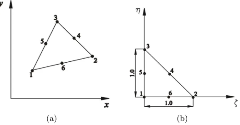
are dependent on the material properties of the two layers adjacent to the i-th interface. The FE formulation of the element has been described in detail in Reference [2]. The element developed may have any arbitrary triangular shape and orientation as shown in Fig. 2(a). It is mapped in a different plane (ζ−η) to have a regular shape as shown in Fig. 2(b).
The stiffness matrix [k], geometric stiffness matrix [kg] and mass matrix [m] are evaluated
for all the elements and assembled together to form the overall stiffness matrix [K], geometric stiffness matrix [KG] and mass matrix [M] of the whole structure and these matrices are stored
in a single array following the skyline storage technique. With these matrices, the equation of equilibrium for an elastic system undergoing small displacements at the instant of buckling may be written as
(a) (b)
Figure 2 A typical element (a) before transformation (b) after transformation.
P =PS+Ptcos Ωt (10)
where PS is the static portion ofP, Pt is the amplitude of the dynamic portion ofP with Ω
as the frequency of excitation. The buckling load Pcr may be used to express PS and Pt as
follows:
PS=αPcr, Pt=βPcr (11)
where α and β are static and dynamic load factors respectively. Using Eqs. (10-11) the equation of motion (9) may be expressed as
[M] {∂¨}+[[K]−αPcr[KG]−βPcr[KG]cos Ωt] {∂}={0}. (12)
Eq. (12) represents a system of second order differential equation with periodic coefficients of Mathieu-Hill type. One of the most interesting characteristics of the equation is that, for certain relationships between its coefficients, it has solution which is unbounded. The regions that correspond to the regions of dynamic instability is the physical problem under consideration in the present study. The boundaries of dynamic instability are formed by the periodic solution of period T and 2T, where T =2π/Ω. The boundaries of the primary instability region with period of 2T are of practical importance and solution can be achieved in the form of trigonometric series:
∂(t)= ∞ ∑ k=1,3,5,...
[{a}ksinkΩt
2 +{b}kcos
kΩt
2 ]. (13)
[[K]−αPcr[KG]±βPcr[KG]−Ω 2
4 [M]] {Υ}={0}. (14)
The two conditions under plus and minus signs correspond to two boundaries (upper and lower) of the dynamic instability region. Eq. (14) is solved by the simultaneous iteration technique proposed by Corr and Jennings [6]. The above eigenvalue solution give the value of Ω, which are the bounding frequencies of the instability regions for the given values of αand
β. Before solving the above equations, the stiffness matrix [K] is modified through imposition of boundary conditions. The boundary conditions used are same as discussed in some earlier studies [2].
3 NUMERICAL EXAMPLES
In this section some numerical examples are presented for imperfect laminated sandwich plates subjected to in-plane partial edge loading. Two different types of loading are considered. In loading type (I), the loaded length in the plate edge is near the corners (see Fig. 3(a)) while in loading type (II), the loaded length is in the middle of the edge (see Fig. 3(b)). In case of uni-axial loading the in-plane edge load is considered to be acting along the x-direction (Fig. 3). As there is no published result on dynamic instability of imperfect as well as perfect laminated sandwich plates subjected to partial edge loading, problem of a perfect isotropic plate subjected to uniform in-plane edge loading is presented for validation. The present results are found to be matching well in this case with the standard results. Subsequently in some cases the present results are compared with those obtained by using the FE package Abaqus (version 6.8). A number of new results are presented for imperfect laminated sandwich plates subjected to partial edge compression, which should be useful in future research.
3.1 Square isotropic plate simply supported at the four edges
To study the convergence and to validate the present results a square isotropic (ν = 0.3) plate simply supported at all the edges having uni-axial in-plane uniform edge loading is analyzed by the present finite element model considering different mesh divisions (4x4, 6x6, 8x8, 12x12, 16x16 and 20x20). It is observed that the convergence in case of thin plate (h/a = 0.01) is obtained for mesh division 16x16. Hence all subsequent analyses are made taking mesh division: 16x16 for the higher thickness ratio (i.e.,h/a= 0.05 and 0.20). The static load factor (α) and the dynamic load factor (β) are varied to identify the lower and upper boundaries of the excitation frequency. The values of the excitation frequency parameters, Ω=ωa2√(
ρh/D)
(a) Loading Type: I
−0.01
(b) Loading Type: II
Figure 3 A rectangular plate (mesh size: m×n) subjected to edge loading.
in the values of the dynamic load factor (i.e., β). This behavior is more prominent in case of thin plates.
3.2 Cross-ply square laminate simply supported at the four edges
The problem of a simply supported cross-ply (0/90/90/0) square laminate (Fig. 3, a = b) subjected to uni-axial in-plane partial edge loading is studied in this example. The analysis is carried out by the proposed element using mesh sizes (full plate) of 10x10 takingh/a = 0.10. In this problem, all the layers are of same thickness and material properties (E1=40E,E2=E,
G12 =G13 = 0.6E, G23 =0.5E and ν12 =0.25). The imperfections at the layer interfaces are defined by the parameters: Rk11=Rk22=Rh/E and Rk12=Rk21=0.0 where the non-dimensional
Table 1 Excitation frequency parameters (Ω) for principal regions of instability of a simply supported square isotropic plate subjected to uniform in-plane edge loading (uni-axial).
h/a β References
Excitation frequency parameters, Ω
α= 0.0 α= 0.20 α= 0.35 Upper Lower Upper Lower Upper Lower 0.01 0.4 Present (4x4) 43.098 35.190 39.343 30.475 36.273 26.392 Present (6x6) 43.167 35.246 39.406 30.524 36.331 26.434 Present (8x8) 43.193 35.267 39.430 30.542 36.353 26.450 Present (12x12) 43.213 35.284 39.448 30.556 36.369 26.463 Present (16x16) 43.224 35.292 39.455 30.562 36.379 26.469 Present (20x20) 43.224 35.292 39.455 30.562 36.379 26.469 Hutt and Salam [9] 43.000 35.320 - - - -Srivastava et al. [15] 43.160 35.370 - - - -0.8 Present (4x4) 46.551 30.475 43.098 24.883 40.315 19.671
Present (6x6) 46.626 30.524 43.167 24.923 40.374 19.703 Present (8x8) 46.654 30.542 43.193 24.938 40.404 19.715 Present (12x12) 46.676 30.556 43.213 24.949 40.422 19.724 Present (16x16) 46.684 30.562 43.221 24.953 40.429 19.727 Present (20x20) 46.684 30.562 43.221 24.953 40.429 19.727 Hutt and Salam [9] 46.560 30.780 - - - -Srivastava et al. [15] 46.540 30.730 - - - -1.2 Present (4x4) 49.765 24.883 46.551 17.595 43.987 8.797
Present (6x6) 49.845 24.923 46.626 17.623 44.057 8.811 Present (8x8) 49.875 24.938 46.654 17.634 44.084 8.817 Present (12x12) 49.899 24.949 46.676 17.642 44.104 8.821 Present (16x16) 49.911 24.956 46.683 17.645 44.116 8.823 Present (20x20) 49.911 24.956 46.683 17.645 44.116 8.823 Hutt and Salam [9] 49.520 25.060 - - - -Srivastava et al. [15] 49.540 24.020 - - - -0.05 0.4 Present (16x16) 42.841 34.980 39.108 30.293 36.056 26.235
0.8 Present (16x16) 46.274 30.293 42.841 24.734 40.074 19.554 1.2 Present (16x16) 49.469 24.734 46.274 17.490 43.724 8.745 0.20 0.4 Present (16x16) 38.222 31.208 34.892 27.027 32.169 23.406
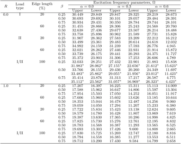
Table 2 Excitation frequency parameters (Ω) of a simply supported square laminated imperfect composite plate (0/90/90/0) subjected to uni-axial in-plane partial edge loading (h/a= 0.10).
R Loadtype Edge length (%) β
Excitation frequency parameters, Ω α= 0.0 α= 0.3 α= 0.6 Upper Lower Upper Lower Upper Lower 0.0 I 20 0.25 30.449 29.849 29.847 29.325 29.219 28.673 0.50 30.693 29.692 30.101 29.057 29.484 28.391 0.75 30.934 29.431 30.350 28.784 29.744 28.101 60 0.25 31.455 28.866 28.306 25.243 24.568 20.760 0.50 32.638 27.436 29.677 23.507 26.214 18.488 0.75 33.758 25.896 30.962 21.589 27.731 15.828 II 20 0.25 31.907 28.362 27.583 23.209 22.212 16.212 0.50 33.499 23.361 29.483 20.614 24.618 12.032 0.75 34.992 24.159 31.239 17.593 26.776 4.945 60 0.25 32.021 28.262 27.446 22.931 21.914 15.872
0.50 33.739 26.175 29.441 20.293 24.375 11.727 0.75 35.372 23.903 31.306 17.253 26.606 4.789 I/II 100 0.25 32.033 28.251 27.432 22.901 21.883 15.838
31.983∗ 28.062∗ 27.155∗ 22.656∗ 21.612∗ 15.623∗
0.50 33.766 26.155 29.436 20.260 24.349 11.697 33.483∗ 25.862∗ 29.055∗ 21.956∗ 23.012∗ 11.423∗
0.75 35.414 23.876 31.313 17.217 26.587 4.775 35.112∗ 23.562∗ 31.057∗ 16.969∗ 26.323∗ 4.423∗
1.0 I 20 0.25 17.207 16.397 16.225 15.311 15.113 14.009 0.50 17.588 15.962 16.647 14.806 15.597 13.304 0.75 17.954 15.503 17.050 14.252 16.051 11.917 60 0.25 17.606 15.960 15.602 13.626 13.185 10.644 0.50 18.353 15.044 16.478 12.487 14.256 9.060 0.75 19.059 14.050 17.294 11.207 15.233 6.380 II 20 0.25 17.722 15.834 15.423 13.138 12.624 9.605 0.50 18.579 14.780 16.428 11.807 13.869 7.619 0.75 19.387 13.630 17.365 10.286 14.998 4.825 60 0.25 17.825 15.730 15.276 12.761 12.195 8.832 0.50 18.783 14.568 16.387 11.293 13.565 6.525 0.75 19.693 13.303 17.426 9.600 14.808 2.665 I/II 100 0.25 17.830 15.725 15.269 12.747 12.180 8.816 0.50 18.794 14.558 16.385 11.277 13.553 6.511 0.75 19.712 13.290 17.430 9.584 14.799 2.658
∗Values indicate results based on Abaqus (Version 6.8)
3.3 Simply supported square sandwich plate having three orthotropic layers
multiple (Kt) of those of the central layer/core where the value of Kt is taken as 5.0. The material properties used for the core areE22/E11=0.543,G12/E11=0.2629,G13/E11=0.1599,
G23/E11 = 0.2668, ν12 = 0.3. The imperfections at the layer interfaces are defined by the parameters: Rk
11=Rk22=Rh/E11 and Rk12=Rk21=0.0 where the non-dimensional parameterR
is varied from 0.0 to 1.2 (R =0.0 represents perfect interface). The uni-axial in-plane partial edge loading is considered for both type I and type II loadings, while α and β are varied as before. The loaded edge length (%) for both the load types are taken as 100 (i.e., fully loaded edge), 60 and 20 respectively. The same loadings are also considered for all subsequent examples. The results obtained for the excitation frequency parameters, Ω=100ω√(ρh2/E11)
are presented in Table 3. Some of the present results (R= 0.0 and 100% in-plane edge loading) are compared here also with the results obtained by using the FE software package Abaqus (version 6.8). The results are quite close to each other in all such cases. In the present case of sandwich plate, it is also observed that the values of both the upper and lower excitation frequencies reduce with increase in the values of imperfection parameter, R. But the rate of reduction is not as high as observed in case of the previous example of laminated composite plate. It is also found that with the increase in the values of loaded edge length the upper excitation frequencies always increase.
3.4 Square sandwich plate with laminated face sheets simply supported at the four edges
The problem of a square simply supported sandwich plate (0/90/C/90/0) having laminated face sheets subjected to in-plane partial edge loading (Fig. 3) is studied in this example for both types of loading (i.e., I and II, Fig. 3). The thickness of the core is 0.8hwhile that of each ply in the laminated face sheets is 0.05h. Taking thickness ratio (h/a) of 0.20, the problem is solved for α = 0.0, 0.3 and 0.6 while β is varied from 0.2 to 0.75. The non-dimensional excitation frequency parameters Ω=100ωa√(ρc/E11)obtained for upper and lower boundary are presented in Table 4. The results show a consistent trend in their variation. The material properties of a ply in the laminated face sheets and those of core are as follows.
Face: E11/E=40.0,E22/E=1.0,G12/E=G13/E=G23/E =1.0, ν12=0.25,ρf =ρ
Core: E/Ec =11.945, Gc12/Ec =Gc13/Ec =1.173/6.279, Gc23/Ec =2.415/6.279, νc12 =0.0025
and ρ/ρc = 0.6818. The imperfections at the layer interfaces are defined by the parameters: Rk11=Rk22=Rh/Ecand Rk12=R21k =0.0 where the non-dimensional parameterR is varied from
0.0 to 1.0.
In this example of a thick plate (h/a= 0.2) it is observed that the difference between the lower and upper excitation frequencies are not so much as observed in the previous examples.
3.5 Sandwich plate under bi-axial in-plane partial edge loading
0.75 16.935 13.678 15.744 11.998 14.414 9.830 60 0.25 16.339 14.453 14.043 11.767 11.253 8.187 0.50 17.199 13.403 15.045 10.433 12.496 6.068 0.75 18.015 12.258 15.980 8.889 13.620 2.489 II 20 0.25 16.327 14.466 14.062 11.824 11.320 8.310 0.50 17.178 13.433 15.050 10.515 12.541 6.221 0.75 17.985 12.307 15.973 9.000 13.646 2.613 60 0.25 16.356 14.436 14.020 11.717 11.198 8.118 0.50 17.236 13.371 15.038 10.372 12.453 6.002 0.75 18.071 12.213 15.991 8.822 13.591 2.454 I/II 100 0.25 16.362 14.430 14.012 11.698 11.178 8.090
16.183∗
14.162∗
13.855∗
11.456∗
11.012∗
7.923∗
0.50 17.247 13.360 15.036 10.348 12.437 5.975 17.083∗
13.162∗
14.955∗
10.058∗
12.212∗
5.723∗
0.75 18.089 12.196 15.995 8.794 13.581 2.439 17.983∗
12.062∗
15.855∗
8.656∗
13.312∗
2.323∗
0.6 I 20 0.25 15.283 14.565 14.415 13.628 13.462 12.578 0.50 15.624 14.186 14.785 13.207 13.871 12.094 0.75 15.955 13.791 15.143 12.763 14.263 11.574 60 0.25 15.792 14.010 13.623 11.479 10.997 8.132
0.50 16.606 13.020 14.569 10.227 12.165 6.182 0.75 17.379 11.941 15.454 8.785 13.224 3.095 II 20 0.25 15.682 14.135 13.803 11.995 11.597 9.322 0.50 16.397 13.288 14.617 10.969 12.567 7.899 0.75 17.081 12.380 15.386 9.825 13.462 5.841 60 0.25 15.828 13.974 13.572 11.348 10.848 7.872 0.50 16.677 12.946 14.555 10.050 12.059 5.827 0.75 17.484 11.827 15.475 8.552 13.158 2.387 I/II 100 0.25 15.836 13.966 13.561 11.321 10.818 7.829 0.50 16.692 12.930 14.552 10.015 12.037 5.782 0.75 17.507 11.803 15.480 8.511 13.143 2.361
(0/90/C/90/0) subjected to uni-axial in-plane partial edge loading (h/a= 0.20).
R Loadtype
Edge length
(%)
β
Excitation frequency parameters, Ω
α= 0.0 α= 0.3 α= 0.6
Upper Lower Upper Lower Upper Lower
0.0 I 20 0.25 22.756 22.217 22.105 21.516 21.391 20.703
0.50 23.014 21.933 22.382 21.197 21.698 20.282 0.75 23.267 21.638 22.651 20.852 21.991 19.680 60 0.25 23.100 21.849 21.582 20.155 19.848 18.179 0.50 23.682 21.171 22.238 19.371 20.601 17.243 0.75 24.238 20.454 22.860 18.532 21.310 14.734
II 20 0.25 23.242 21.698 21.369 19.601 19.220 17.134
0.50 23.955 20.861 22.179 18.628 20.154 15.918 0.75 24.635 19.972 22.946 17.580 21.032 11.891 60 0.25 23.587 21.334 20.853 18.248 17.679 14.492 0.50 24.633 20.108 22.036 16.789 19.068 12.579 0.75 25.632 18.799 23.155 15.185 20.360 6.781
I/II 100 0.25 23.661 21.256 20.741 17.949 17.336 13.875
0.50 24.776 19.944 22.005 16.375 18.830 11.768 0.75 25.843 18.541 23.200 14.633 20.213 6.568
0.5 I 20 0.25 15.472 15.209 15.155 14.879 14.822 14.525
0.50 15.600 15.074 15.289 14.735 14.963 14.368 0.75 15.725 14.935 15.420 14.586 15.101 14.202 60 0.25 15.711 14.958 14.800 13.969 13.794 12.864 0.50 16.067 14.558 15.190 13.525 14.226 12.359 0.75 16.411 14.141 15.565 13.058 14.640 11.278
II 20 0.25 15.783 14.883 14.694 13.696 13.485 12.356
0.50 16.207 14.404 15.160 13.160 14.005 11.727 0.75 16.616 13.903 15.608 12.593 14.501 10.029 60 0.25 15.977 14.677 14.403 12.939 12.626 10.917 0.50 16.588 13.980 15.080 12.139 13.396 9.941 0.75 17.176 13.245 15.726 11.280 14.123 5.622
I/II 100 0.25 16.026 14.626 14.330 12.745 12.404 10.533
0.50 16.681 13.873 15.059 11.873 13.240 9.460 0.75 17.312 13.077 15.756 10.933 14.027 4.212
1.0 I 20 0.25 12.504 12.204 12.143 11.823 11.757 11.410
0.50 12.649 12.049 12.296 11.656 11.921 11.223 0.75 12.791 11.889 12.445 11.482 12.080 11.023 60 0.25 12.750 11.943 11.772 10.862 10.667 9.614
0.50 13.128 11.510 12.193 10.366 11.146 9.023 0.75 13.490 11.052 12.595 9.837 11.598 6.852
II 20 0.25 12.811 11.878 11.681 10.622 10.395 9.152
0.50 13.246 11.376 12.168 10.042 10.953 8.432 0.75 13.663 10.844 12.632 9.417 11.478 4.464 60 0.25 12.898 11.788 11.553 10.295 10.025 8.538 0.50 13.417 11.191 12.132 9.603 10.689 7.683 0.75 13.917 10.559 12.684 8.856 11.313 3.526
I/II 100 0.25 12.924 11.760 11.514 10.191 9.906 8.331
Table 5 Excitation frequency parameters (Ω) of square laminated imperfect sandwich plate (-45/45/C/45/-45) under bi-axial in-plane partial edge loading (h/a= 0.10).
R Loadtype Edge length (%) β
Excitation frequency parameters, Ω α= 0.0 α= 0.3 α= 0.6 Upper Lower Upper Lower Upper Lower 0.0 I 20 0.20 21.551 20.498 19.922 18.630 17.881 16.009 0.60 22.508 19.304 21.038 17.028 19.304 12.550 0.75 22.847 18.804 21.425 16.284 19.772 7.952 60 0.20 21.703 20.344 19.613 18.010 17.108 14.939
0.60 22.958 18.839 21.038 16.103 18.839 11.271 0.75 23.406 18.223 21.539 15.250 19.424 7.055 II 20 0.20 21.574 20.478 19.890 18.616 17.921 16.376
0.60 22.580 19.270 21.038 17.178 19.270 14.512 0.75 22.937 18.783 21.442 16.583 19.738 13.595 60 0.20 21.811 20.230 19.381 17.526 16.499 14.144 0.60 23.264 18.483 21.038 15.382 18.483 10.984 0.75 23.782 17.772 21.621 14.467 19.161 8.234 I/II 100 0.20 21.951 20.083 19.079 16.884 15.666 12.864
0.60 23.668 18.016 21.038 14.338 18.016 9.120 0.75 24.280 17.174 21.726 13.249 18.819 6.736 0.5 I 20 0.20 15.791 14.997 14.562 13.576 12.999 11.524
0.60 16.509 14.092 15.405 12.332 14.092 8.704 0.75 16.764 13.710 15.696 11.744 14.448 5.308 60 0.20 15.918 14.868 14.302 13.052 12.341 10.593
0.60 16.883 13.700 15.405 11.540 13.700 7.477 0.75 17.228 13.219 15.792 10.848 14.156 4.310 II 20 0.20 15.747 15.049 14.677 13.880 13.451 12.517
0.60 16.394 14.288 15.405 12.998 14.288 11.435 0.75 16.625 13.984 15.663 12.640 14.581 10.674 60 0.20 16.006 14.774 14.108 12.643 11.824 9.921
3.6 Simply supported double core rectangular sandwich plate with laminated stiff sheets
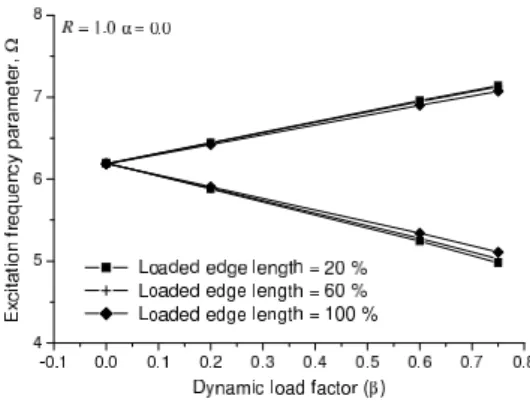
The problem of a simply supported rectangular sandwich plate having double core with three laminated stiff sheets (0/90/90/0/C/0/90/90/0C/0/90/90/0) is studied in this example taking uni-axial in-plane partial edge loading (Type I). The thickness of each core is 0.425h while that of each ply in the stiff laminated sheets is 0.0125h. Their material properties and the imperfections at the layer interfaces are same as those used in the previous example. In this example, the plate subjected to uni-axial in-plane partial edge loading is analyzed with the proposed FE model with aspect ratio (a/b) = 2.0 and thickness ratio (h/a) = 0.20 for different values of imperfection parameter (R). In this example by varying α and β from 0 to higher values the full range of dynamic instability is studied. For all these cases, the excitation frequency parameter Ω=100ωa√(ρc/E11)obtained are presented in Figures 4–12. The figures
(4-12) show the locations of the tips (i.e., β = 0.0) of the whole dynamic stability regions, which also shows the difference between the stability and instability regions It is observed from the results shown in the figures (4-12) that for higher values ofαandβthe uniform trend is disturbed in some cases.
Figure 4 Instability region of a simply supported double core laminated sandwich plate (R=0.0,α=0.0).
Figure 6 Instability region of a simply supported double core laminated sandwich plate (R=0.0,α=0.6).
Figure 7 Instability region of a simply supported double core laminated sandwich plate (R=0.5,α=0.0).
Figure 9 Instability region of a simply supported double core laminated sandwich plate (R=0.5,α=0.6).
Figure 10 Instability region of a simply supported double core laminated sandwich plate (R=1.0,α=0.0).
Figure 12 Instability region of a simply supported double core laminated sandwich plate (R=1.0,α=0.6).
4 CONCLUSIONS
In this paper the dynamic instability characteristics of imperfect laminated sandwich plate subjected to in-plane partial edge loading is carried out by an efficient finite element plate model. The present finite element model has all the necessary features for an accurate model-ing of the present problem while it is computationally as elegant as any smodel-ingle layer plate. As there is no investigation on dynamic instability of imperfect laminated sandwich plate using such a refined plate model, a number of problems are solved including different plate geometry, boundary conditions, stacking sequences, thickness ratio and other aspects. In general it may be observed that the dynamic instability region is more expanded in case of 100% (i.e. full) loaded edge length. Also with the increase in the imperfection parameter (R) the dynamic in-stability region is contracted and the effect of different loaded edge length is gradually reduced. In this process many results are generated, which should be helpful for future research.
References
[1] V. V. Bolotin. The Dynamic stability of Elastic systems. Holden-Day, San Francisco, 1964.
[2] A. Chakrabarti and A. H. Sheikh. Vibration of composites and sandwich laminates subjected to in-plane partial edge loading.Comp. Sc. Tech., 67:1047–1057, 2007.
[3] A. Chakrabarti and A. H. Sheikh. Dynamic instability of composite and sandwich laminates with interfacial slips.
International Journal of Structural Stability and Dynamics, 10(2):205–224, 2010.
[4] A. Chattopadhyay and A. G. Radu. Dynamic instability of composite laminates using a higher order theory.Computer and Structure, 77:453–460, 2000.
[5] L. W. Chen and J. Y. Yang. Dynamic stability of laminated composite plates by the finite element method.Computer and Structure, 36:845–851, 1990.
[6] R. B. Corr and A. Jennings. A simultaneous iteration algorithm for symmetric eigenvalue problems. International Journal Numerical Methods Engineering, 10:647–663, 1976.
[7] P. J. Deolasi and P. K. Datta. Parametric instability of rectangular plates subjected to localized edge compressing (compression or tension). Computer and Structure, 54:73–82, 1995.
[8] J. Fazilati and H. R. Ovesy. Dynamic instability analysis of composite laminated thin-walled structures using two versions of FSM. Composite Structures, 92(9):2060–2065, 2010.
[10] K. S. Jagdish. The dynamic stability of degenerate systems under parametric excitation. Ingenieur-Archive, 43:240– 246, 1974.
[11] Y. W. Kwon. Finite element analysis of dynamic instability of layered composite plates using a high-order bending theory. Computer and Structure, 38:57–62, 1991.
[12] S. Y. Lee. Finite element dynamic stability analysis of laminated composite skew plates containing cutouts based on HSDT. Composite Science & Technology, 70(8):1249–1257, 2010.
[13] S. V. Patel, P. K. Datta, and A. H. Sheikh. Parametric study on the dynamic instability behavior of laminated composite stiffened plate. Journal of Engineering Mechanics ASCE, 135(11):1331–1341, 2009.
[14] R. S. Srinivasan and P. Chellapandi. Dynamic stability of rectangular laminated composite plates. Computer and Structure, 24:233–238, 1986.
[15] A. K. L. Srivastava, P. K. Datta, and A. H. Sheikh. Dynamic instability of stiffened plates subjected to non-uniform harmonic edge loading. Journal of Sound and Vibration, 262:1171–1189, 2003.