Behavior analysis of bar gaps in welded YT-joints for rolled-steel
circular hollow sections
Abstract
We present a parametric analysis of gap variation between the lap brace and through brace of YT welded joints for rolled-steel circular hollow sections on plane steel structures. Our aim is to investigate the collapse behavior of YT-joints under lap brace axial compression. In particular, we focus one/d0 ratios above 0.25 so bending moments can be taken
into account during the design. We find that joint failure is primarily due to chord wall plastification (Mode A) and cross-sectional chord buckling (Mode F) in the region un-derneath the lap brace. Our joint design followed the Limit States Method, and our results were based on a comparative analysis of three different methods: an analytical solution derived from a set of international technical norms, an ex-perimental analysis, and numerical modeling using Ansys as calibrated by our experimental results.
Keywords
Circular hollow sections, joint, bar gap, finite-element anal-ysis, parametric study.
R.F. Vieiraa,∗, J.A.V. Requenaa,
A. M. S. Freitasb and
V. F. Arcaroa
aState University of Campinas, Campinas, SP
– Brazil
bFederal University of Ouro Preto, Ouro Preto,
MG – Brazil
Received 12 Mar 2010; In revised form 8 Dez 2010
∗Author email: [email protected]
1 INTRODUCTION
The extensive use of steel frame structures is primarily due to the economic advantages of manufacturing steel frames. In this work, we study the strength of connection joints for tubular steel frames as a function of gap length between the lap and through braces of YT-joints. This work extends earlier studies of tubular joints that focused on experimental tests [5], theoretical analyses using the Finite Element Method [2–4], and analytical work aimed at developing mathematical expressions of the joint strength [6].
2 CALCULATION OF CONNECTION RESISTANCE
The YT joint prototype design uses the methodology presented by Wardenier et al. [10] and Packer and Henderson [7].
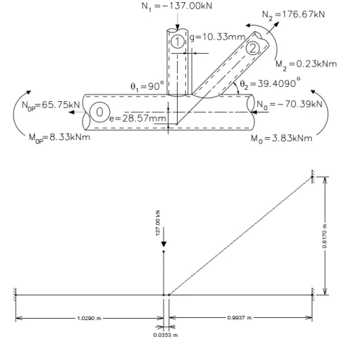
M0 bending moment in the chord member; Ni axial force applied to memberi(i=0,1,2,3);
Ni∗ joint design resistance expressed in terms of axial load in member i; N0P pre-stressing axial force on the chord;
W0 elastic section modulus of memberi(i=0,1,2,3);
di external diameter of circular hollow section for member i(i=0,1,2,3);
e nodding eccentricity for a connection; fy yield stress;
fyi yield stress of memberi (i=0,1,2,3);
f0P pre-stress in chord;
f(n′) function which incorporates the chord pre-stress in the joint resistance equation;
g gap between the bracings members of a K, N or KT joint, at the face of the chord;
g′ gap divided by chord wall thickness;
n′ f0P
fy0
= N0P
A0⋅fy0 +
M0
W0⋅fy0
ti thickness of hollow section member i(i=0,1,2,3);
β diameter ratio between bracing on chord; β =d1
d0,
d1
b0,
bi
b0 T, Y and X
β =d1+d2
2⋅d0 ,
d1+d2
2⋅b0 ,
b1+b2+h1+h2
4⋅b0 K and N
γ ratio of the chord’s half diameter to its thickness; ν Poisson’s ratio
θ included angle between bracing member i(i=0,1,2,3) and the chord;
ϵ maximum specific proportionality strain;
f stress;
flp maximum proportionality stress;
fr maximum resistance stress;
f1 principal stress 1; f2 principal stress 2;
Table 1 shows the geometric characteristics of the VMB 250 circular hollow sections used in the YT joint. The nominal physical proprieties yield stress (fy) are equal 250 MPa.
2.1 Validity limits
Figure 1 Forces general scheme of YT joint.
Table 1 Physical and geometrical characteristics.
Member Hollow Section Thickness Area
Elastic resistant modulus
Load
mm mm mm2
mm3
kN
Chord ϕ114.3 #6.02 2047.83 52677.51 N0= - 70.39
N0P = 65.75
Lap brace ϕ73.0 #5.16 1099.73 17433.30 N1= -137.00
Through
β= d1+d2
2⋅d0 ; (1)
g′= g
t0; (2)
The stress on the chord, f0P, depends most critically on the compressing stress.
n′= f0P
fy0
= N0P
A0⋅fy0+ M0 W0⋅fy0
; (3)
f (n′)=1.0+0.3⋅n′ − 0.3⋅n′2 ≤ 1 ; (4)
f (γ, g′)=γ0.2⋅(1+ 0.024⋅γ
1.2
1+exp(0.5⋅g′−1.33)); (5)
B) Plastic failure of the chord face (Mode A)
Vertical lap brace:
N1∗= fy0⋅t
2 0
senθ1 (1.8+10.2⋅ d1
d0) ⋅f (γ, g
′)
⋅ f (n′); (6)
Diagonal through brace:
N2∗=N1∗ ⋅( senθ1
senθ2); (7)
C) Punching shear failure of the chord face (Mode B)
Vertical lap brace and diagonal through brace are both given by Eq. (8):
Ni∗= fy0⋅t0√⋅π⋅di
3 ⋅ (
1+senθi
2⋅sen2θ
i)
; (8)
D) YT Joint Resistance
The joint resistance is the lowest value obtained in items (B) and (C) above. Vertical lap brace:
N1 N∗
1
<1; (9)
N2 N2∗
<1; (10)
Table 2 presents the results of the calculation.
Table 2 Results of the calculation procedure.
Joint parameters Acronym Calculation
Relation between diameters β 0.64
Relation between diameter and thickness γ 9.49
n′ = stress/fy (compression) n′ -0.14
Function of prestress on chord f(n′) 0.95
Resistance plastic failure of the chord face (Mode A) N1∗(P l) 137.40 kN Resistance punching shear failure of the chord face (Mode B) N1∗(P u) 199.27 kN
Lap brace use N1/N1∗ 1.0
Resistance plastic failure of the chord face (Mode A) N2∗(P l) 216.42 kN Resistance punching shear failure of the chord face (Mode B) N2∗(P u) 404.16 kN
Through brace use N2/N2∗ 0.82
3 EXPERIMENTAL PROGRAM
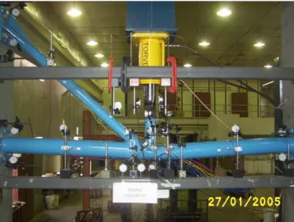
To study the joint, four prototypes constructed from seamless rolled tubes were manufactured by V&M do Brasil. They were called pre-experiment, experiments I, II and III [9].
3.1 YT joint prototypes
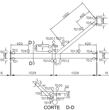
The dimensions of the prototypes are shown in Fig. 2. The prototypes are fixed by four screws at each end. They were loaded axially at the top of the lap brace.
3.2 Instrumentation for tests
In EXPERIMENTS I, II and III, sixteen 5mm electrical resistance KFG-5-120-C1-11 exten-someters were used. Their positions are marked EER1 to EER16 in Fig. 3.
The EERs were placed on the prototype to measure longitudinal strain, drawing on the work of Fung et al [5]. In EXPERIMENT III, 2 rosette gauges and 2 individual extensometers were added (for a total of 24 EERs). Rosette 1 was composed of EER20, EER21 and EER22; rosette 2 was composed of EER17, EER18 and EER19. EER23 and EER24 were placed at the bases of the lap brace and through brace respectively.
Figure 2 YT joint prototype (mm).
Figure 3 Positioning of the extensometers on the YT joint prototype.
3.3 Experimental results
The testing methodology used was defined in three stages, as shown below:
Stage I. Before starting the test, the prototype was subjected to a cycle of 10 loading of approximately 20% of the estimated collapse loading for the connection, to minimize friction and check the torque of the screws. Based on pre-test the loading was estimated at 50kN. This level of loading is within the elastic limit of the material. The force was applied in small increments and then it was done downloading.
Figure 4 Positioning of the DTs on the YT joint prototype.
for both the case of loading and for unloading. The step load was previously set depending on the stage supposed to loading. At each step of loading, when the pre established loading was reached, expected time to stabilize the transducers and then did the reading.
Stage III. The prototype was loaded to the ultimate state, where the prototype did not offer more resistance, even after he reached the break. Then the prototype was unloaded.
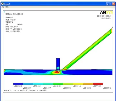
Fig. 5 shows the overall strain of the prototype in EXPERIMENT III, characterized by the development of failure Mode A.
The results presented by extensometers in each EXPERIMENTS I, II and III are similar, are representing the state of tension expected for each region and thus show that the tests were equivalent.
The results of the last loading for each of the tests are shown in Table 3.
Table 3 Last loading to EXPERIMENTS I, II and III.
EXPERIMENTS
Last loading
(kN)
EXPERIMENT I 240.0
EXPERIMENT II 358.6
Figure 5 Overall strain of the prototype for EXPERIMENT III.
Two failure modes were observed: plastic failure of the chord face (Mode A) and local buckling of the chord walls (Mode F).
4 ANALYSIS OF FINITE ELEMENTS
Two numerical models were created in Ansys [1], one using a bilinear stress-strain diagram (BISO – Bilinear Isotropic Hardening) and the other a multilinear (piecewise linear) diagram (MISO – Multilinear Isotropic Hardening). Their results were compared to the experimental tests [9].
Both physical and geometrical non-linearity were considered in the analysis. To implement physical non-linearity, we used the stress-strain diagrams obtained through test-body traction. Test bodies cp1a, cp1b for hollow section of diameter 73mm and cp2a e cp2b for hollow section of diameter 114.3mm [9].
The contour conditions were simulated in Ansys through displacement restrictions. Force was applied in an increasing way, that is, at unit load pitches.
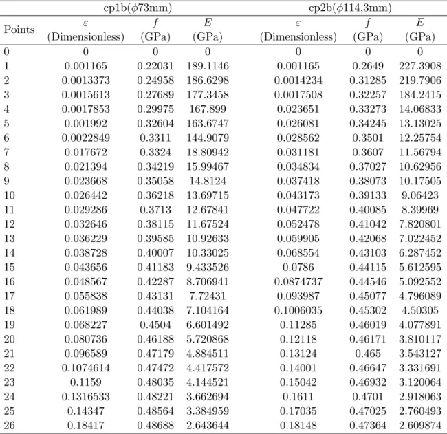
Fig. 6 and Fig. 7 show the stress-strain diagrams of test bodies selected for the numerical analysis. The multilinear model is represented by 26 points (crossed circles), and the bilinear model by two straight lines (triangles).
Table 4 shows data used to represent the material properties of test bodies cp1b and cp2b in the numerical model. Note that the bilinear stress-strain diagram always runs from the origin to the first stress peak (f), then from this point to the maximum stress (fr) of the
material.
Figure 6 Experimental, bilinear and multilinear stress-strain diagrams used for test body cp1b, from the through brace and lap brace (φ73mm).
Figure 7 Experimental, bilinear and multilinear stress-strain diagrams used for test body cp2b, from the chord (φ114.3mm).
Table 4 Data used to represent the bilinear stress-strain diagram with the Ansys software (BISO).
Test Body fy f fr E Et
(MPa) (MPa) (MPa) (MPa) (MPa)
cp1b(ϕ73mm) 326.0 331.1 486.9 189114.6 856.5
Table 5 Data used to represent the multilinear stress-strain diagram with the Ansys software (MISO).
cp1b(ϕ73mm) cp2b(ϕ114,3mm)
Points ε f E ε f E
(Dimensionless) (GPa) (GPa) (Dimensionless) (GPa) (GPa)
0 0 0 0 0 0 0
1 0.001165 0.22031 189.1146 0.001165 0.2649 227.3908
2 0.0013373 0.24958 186.6298 0.0014234 0.31285 219.7906
3 0.0015613 0.27689 177.3458 0.0017508 0.32257 184.2415
4 0.0017853 0.29975 167.899 0.023651 0.33273 14.06833
5 0.001992 0.32604 163.6747 0.026081 0.34245 13.13025
6 0.0022849 0.3311 144.9079 0.028562 0.3501 12.25754
7 0.017672 0.3324 18.80942 0.031181 0.3607 11.56794
8 0.021394 0.34219 15.99467 0.034834 0.37027 10.62956
9 0.023668 0.35058 14.8124 0.037418 0.38073 10.17505
10 0.026442 0.36218 13.69715 0.043173 0.39133 9.06423
11 0.029286 0.3713 12.67841 0.047722 0.40085 8.39969
12 0.032646 0.38115 11.67524 0.052478 0.41042 7.820801
13 0.036229 0.39585 10.92633 0.059905 0.42068 7.022452
14 0.038728 0.40007 10.33025 0.068554 0.43103 6.287452
15 0.043656 0.41183 9.433526 0.0786 0.44115 5.612595
16 0.048567 0.42287 8.706941 0.0874737 0.44546 5.092552
17 0.055838 0.43131 7.72431 0.093987 0.45077 4.796089
18 0.061989 0.44038 7.104164 0.1006035 0.45302 4.50305
19 0.068227 0.4504 6.601492 0.11285 0.46019 4.077891
20 0.080736 0.46188 5.720868 0.12118 0.46171 3.810117
21 0.096589 0.47179 4.884511 0.13124 0.465 3.543127
22 0.1074614 0.47472 4.417572 0.14001 0.46647 3.331691
23 0.1159 0.48035 4.144521 0.15042 0.46932 3.120064
24 0.1316533 0.48221 3.662694 0.1611 0.4701 2.918063
25 0.14347 0.48564 3.384959 0.17035 0.47025 2.760493
ν = 0.3.
The SHELL element was considered most appropriate to represent hollow structures. Specifically, the SHELL181 element was used to generate a mesh for the hollow sections. The SHELL63 element was used for fixation plates. Table 6 shows their characteristics.
Table 6 Characteristics of elements.
Elements Nr of nodes per element
Degrees of
freedom Special features
SHELL 63 4 6 Elastic Large deflection Little strain
SHELL 181 4 6 Plastic Large deflection Large strain
5 COMPARISON BETWEEN EXPERIMENTAL TEST RESULTS AND NUMERICAL
MODEL RESULTS
The experimental tests and numerical models can be compared on the basis of strains obtained by the extensometers [9].
For the rosettes, comparisons between theory and experiment can be made between the principal stresses.
Fig. 8 show the principal stresses f1 measured at rosette 1 in EXPERIMENT III and the numerical models.
6 METHODS USED FOR PARAMETRIC ANALYSIS
Summarizing, the overall geometry and minimum allowable gap size of the YT-joint described in this work is shown in Fig. 2. Using this schematic, we fabricated and tested four test specimens in the laboratory and generated numerical models using program Ansys. Our nu-merical models were calibrated using our experimental results, so as to precisely represent the predefined gap in the YT-joint [9]. These models used a SHELL181 four-node element for the tubular sections, and we took into account both material and geometric nonlinearity effects [8], the latter using a Multilinear Isotropic Hardening (MISO) material.
We performed a parametric analysis to study the effect of gap size between the lap brace and through brace on the overall strength of the YT-joint. The motivation for this study stems from the observation that the gap length can influence the resistance to chord wall plastification failure (Mode A) for YT-joints using circular hollow sections.
According to Packer and Henderson [7], the e/d0 ratio for the joint must satisfy the limits given by Eq. (11); this represents the range over which the effects of the joint’s bending moments can be disregarded, namely.
−0.55≤( e
d0)≤0.25. (11)
If these eccentricity boundaries are exceeded, then the generated moment has a detrimental effect on the joint strength since the moment must be distributed between the braces. If this occurs, the joint capacity must be checked for interaction between the axial force and the bending moment.
Note that for gap lengths greater than the lowest acceptable value ofg=10.33 mm, we have g≥t1+t2and thee/d0 ratio exceeds the boundary condition of 0.25. Consequently, this work
will focus one/d0ratios between 0.25 and 0.97 when analyzing new models. Our overall focus is to study the strength YT-joints for gap lengths greater than g=10.33 mm, with emphasis on the influence of bending moments on the overall joint design.
7 GAP LENGTH MODELS
Table 7 shows the gap lengths studied here, along with their corresponding eccentricity “e” values and e/d0 ratios.
Gap Lengths (mm) e (mm) e/d0 gap=10.33 (GAP10.33) 28.57 0.25
gap =30 (GAP30) 44.73 0.39
gap=50 (GAP50) 61.17 0.54
gap=70 (GAP70) 77.60 0.68
gap=90 (GAP90) 94.03 0.82
gap=110 (GAP110) 110.47 0.97
8 RESULTS FOR THE EFFECT OF GAP LENGTH ON YT-JOINT STRENGTH
The principal stresses “f1” for each gap size are shown in Figs. 9 through 14. For all models, the largest stresses were observed on the chord at the joint intersection.
Figure 9 Principal stress “f1” for model “GAP10.33”.
Our models show that the stress distributions between the lap brace and through brace are indeed influenced by the gap size. As seen in Fig. 15, varying gap sizes from the “GAP10.33” to “GAP110” models produces approximately twice the principal stress “f1” for the same load of 100kN.
For each model, the respective yield load was then determined based on a yield strength of σe = 0.33 GPa, as defined by a tensile test [8]. Table 8 shows the yield load for each of the
Figure 10 Principal stress “f1” for model “GAP30”.
Figure 12 Principal stress “f1” for model “GAP70”.
Figure 14 Principal stress “f1” for model “GAP110”.
Gap Length (mm) Yield Load (kN)
gap=10.33 (GAP10.33) 161
gap=30 (GAP30) 131
gap=50 (GAP50) 121
gap=70 (GAP70) 115
gap=90 (GAP90) 109
gap=110 (GAP110) 104
8.1 Failure modes
The predominant failure modes for “GAP30” through “GAP110” are shown in Figs. 16 through 19, respectively. This shows that the main failure mechanisms are due to chord wall plastifi-cation (Mode A) and chord buckling (Mode F).
Figure 16 Plastic failure due to chord wall plastification in model “GAP30”.
9 NUMERICAL ANSYS ANALYSIS OF DIMENSION LOAD VERSUS YIELD LOAD
We designed the tubular YT-joint specimen using values presented by CIDECT [10] and Packer and Henderson [7]. This gave a dimension load of 137 kN with 100% efficiency on the top of the lap brace and 82% efficiency for the through brace (Item 2). Note that we did not take bending moments into consideration during the design calculations sincee/d0=0.25.
Figure 17 Chord buckling in model “GAP30”.
Figure 19 Chord buckling in model “GAP110”.
of the new models were calculated in the same way as before, except that we took bending moments into consideration since e/d0 >0.25. We compared the results with the yield loads
supplied by Ansys, and our results are presented in Fig. 20.
Table 9 shows the values of dimension load, yield load and the percent difference between them.
Table 9 Dimension load, yield load and percent difference between them.
Gap Model
Dimension Load
Yield Load
(kN) Percent
Difference
(kN) Ansys
GAP10.33 137 161 17.52%
GAP30 114 131 14.91%
GAP50 112 121 8.04%
GAP70 113 115 1.77%
GAP90 111 109 -1.80%
0 20 40 60 80 100 120 140
0 10 20 30 40 50 60 70 80 90 100 110 120
Gap (mm) L a p b ra c e a x ia l c o m p re s s
Yield load (ANSYS)
Dimension load - With bending moment (Mode A) Dimension load - Without bending moment (Mode A)
Figure 20 Dimension load and yield load.
10 CONCLUSIONS
We found that variation in gap lengths do not alter the principal failure mode for YT-joints. The principal failure modes are due to wall chord plastification (Mode A) and chord buckling (Mode F) regardless of the gap length. For gap lengths betweeng=10.33 mm andg=110 mm, the percent difference between the dimension load and the yield load decreases as the gap length increases. For gap values up to g=70 mm, the yield load of the numerical model is above the dimension load, implying that such designs are safe. For gap lengths greater than g=70 mm, the yield load falls short of the dimension load, implying that such designs are unsafe and the existing formulations of such joint designs should be reexamined.
Acknowledgements The authors are grateful for the support from UNICAMP, from Vallourec & Mannesmann Tubes (V&M do Brasil).
References
[1] ANSYS. Inc. Theory reference, version 9.0. 2004.
[2] E. M. Dexter and M. M. K. Lee. Static strength of axially loaded tubular K-joint. I: Behaviour.Journal of Structural
Engineering, 125(2):194–201, 1999.
[3] E. M. Dexter and M. M. K. Lee. Static strength of axially loaded tubular K-joint. II: Ultimate capacity. Journal of
Structural Engineering, 125(2):202–210, 1999.
[4] T. C. Fung, C. K. Soh, and W. M. Gho. Ultimate capacity of completely overlapped tubular joints – II. Behavioural study. Journal of Constructional Steel Research, 57(8):881–906, 2001.
Engineering, 110(2):385–400, 1984.
[7] J. A. Packer and J. E. Henderson. Hollow structural section connections and trusses: a design guide. Canadian Institute of Steel Construction, Ontario, 2nd edition, 1997.
[8] R. F. Vieira. Um estudo sobre ligaes do tipo YT de barras afastadas de sees tubulares circulares laminadas de a¸co. PhD thesis, Estruturas, Universidade Estadual de Campinas, Campinas, 2007.
[9] R. F. Vieira, J. A. V. Requena, A. M. S. Freitas, and V. F. Arcaro. Numerical and experimental analysis of yield loads in welded gap hollow YT-joint. Latin American Journal of Solids and Structures, 6(4):363–383, 2009.
[10] J. Wardenier, Y. Kurobane, J. A. Packer, D. Dutta, and N. Yeomans.Design guide for circular hollow section (CHS)