Air–snow transfer of nitrate on the East Antarctic Plateau – Part 2: An isotopic model for the interpretation of deep ice-core records

www.atmos-chem-phys.net/15/12079/2015/ doi:10.5194/acp-15-12079-2015

© Author(s) 2015. CC Attribution 3.0 License.

Air–snow transfer of nitrate on the East Antarctic Plateau – Part 2:

An isotopic model for the interpretation of deep ice-core records

J. Erbland1,2, J. Savarino1,2, S. Morin3, J. L. France4,a, M. M. Frey5, and M. D. King4

1_{Université Grenoble Alpes, LGGE, 38000 Grenoble, France} 2_{CNRS, LGGE, 38000 Grenoble, France}

3_{Météo-France – CNRS, CNRM – GAME UMR 3589, CEN, Grenoble, France}

4_{Department of Earth Sciences, Royal Holloway University of London, Egham, Surrey, TW20 0EX, UK} 5_{British Antarctic Survey, Natural Environment Research Council, Cambridge, UK}

a_{now at: School of Environmental Sciences, University of East Anglia, Norwich, NR4 7TJ, UK}

Correspondence to:J. Savarino (joel.savarino@ujf-grenoble.fr)

Received: 9 January 2015 – Published in Atmos. Chem. Phys. Discuss.: 10 March 2015 Revised: 1 September 2015 – Accepted: 7 September 2015 – Published: 30 October 2015

Abstract. Unraveling the modern budget of reactive nitro-gen on the Antarctic Plateau is critical for the interpretation of ice-core records of nitrate. This requires accounting for nitrate recycling processes occurring in near-surface snow and the overlying atmospheric boundary layer. Not only con-centration measurements but also isotopic ratios of nitrogen and oxygen in nitrate provide constraints on the processes at play. However, due to the large number of intertwined chemical and physical phenomena involved, numerical mod-eling is required to test hypotheses in a quantitative manner. Here we introduce the model TRANSITS (TRansfer of At-mospheric Nitrate Stable Isotopes To the Snow), a novel con-ceptual, multi-layer and one-dimensional model representing the impact of processes operating on nitrate at the air–snow interface on the East Antarctic Plateau, in terms of concen-trations (mass fraction) and nitrogen (δ15N) and oxygen iso-topic composition (17_{O excess,1}17_{O) in nitrate. At the air–}

snow interface at Dome C (DC; 75◦₀₆′_{S, 123}◦₁₉′_{E), the} model reproduces well the values ofδ15N in atmospheric and surface snow (skin layer) nitrate as well as in theδ15N profile in DC snow, including the observed extraordinary high pos-itive values (around+300 ‰) below 2 cm. The model also captures the observed variability in nitrate mass fraction in the snow. While oxygen data are qualitatively reproduced at the air–snow interface at DC and in East Antarctica, the sim-ulated 117O values underestimate the observed 117O val-ues by several per mill. This is explained by the simplifi-cations made in the description of the atmospheric cycling

and oxidation of NO2as well as by our lack of

understand-ing of the NOxchemistry at Dome C. The model reproduces well the sensitivity ofδ15N,117O and the apparent fractiona-tion constants (15εapp,17Eapp) to the snow accumulation rate.

Building on this development, we propose a framework for the interpretation of nitrate records measured from ice cores. Measurement of nitrate mass fractions andδ15N in the ni-trate archived in an ice core may be used to derive informa-tion about past variainforma-tions in the total ozone column and/or the primary inputs of nitrate above Antarctica as well as in nitrate trapping efficiency (defined as the ratio between the archived nitrate flux and the primary nitrate input flux). The 117O of nitrate could then be corrected from the impact of cage recombination effects associated with the photolysis of nitrate in snow. Past changes in the relative contributions of the117O in the primary inputs of nitrate and the117O in the locally cycled NO2and that inherited from the additional

O atom in the oxidation of NO2could then be determined.

1 Introduction

Ice cores from the East Antarctic Plateau provide long-term archives of Earth’s climate and atmospheric composition such as past relative changes in local temperatures and global atmospheric CO2levels (EPICA community members, 2004,

for example). Soluble impurities have been used in such cores as tracers of biogeochemical processes. As the end product of the atmospheric oxidation of NOx (NO+NO2),

nitrate (NO−₃)is a major ion found in Antarctic snow (Wolff, 1995). Its primary origins are a combination of inputs from the stratosphere and from low-latitude sources (Legrand and Delmas, 1986; Legrand and Kirchner, 1990). Stratospheric inputs of nitrate are believed to be mostly caused by the sedi-mentation of polar stratospheric clouds (PSCs) in winter (Se-infeld and Pandis, 1998; Jacob, 1999). The interpretation of nitrate deep ice-core records remains elusive (e.g., Wolff et al., 2010), mainly because its deposition to the snow is not irreversible (Traversi et al., 2014, and references therein) at low-accumulation sites such as Dome C or Vostok (78◦27′S, 106◦50′E; elevation 3488 m a.s.l.).

Nitrate loss from snow can occur through the physical re-lease of HNO3(via evaporation and/or desorption, also

re-ferred to as simply “evaporation”) or through the UV photol-ysis of the NO−₃ ion (Röthlisberger et al., 2000). At wave-lengths (λ) below 345 nm, NO−₃ photolyzes to form NO2

(Chu and Anastasio, 2003) or NO−₂ ion (Chu and Anasta-sio, 2007), which can form HONO at pH<7. Nitrate pho-tolysis is quantitatively represented by its rate constant (J ) expressed as follows:

J =

Z

8 (λ, T ) σ (λ, T ) I (λ, θ, z)dλ, (1) with8the quantum yield,σ the absorption cross section of NO−₃,I the actinic flux,λthe wavelength,T the temperature, θ the solar zenith angle andzthe depth. Two recent labora-tory studies have investigated nitrate photolysis in Dome C (DC; 75◦06′S, 123◦19′E) snow. Meusinger et al. (2014) re-ported the quantum yields for the photolysis of either photo-labile or buried nitrate. The terms “photophoto-labile” and “buried” were introduced by Meusinger et al. (2014) as different “do-mains”, i.e., different physicochemical properties of the re-gion around the nitrate chromophore. Berhanu et al. (2014a) reported the absorption cross section of14NO−₃ and15NO−₃ in Antarctic snow at a given temperature, using a new semi-empirical zero-point energy shift (1ZPE) model.

Nitrate deposition to the snow can occur through vari-ous mechanisms, including co-condensation and dry depo-sition (Röthlisberger et al., 2000; Frey et al., 2009). Within the snowpack, nitrate can be contained as HNO3 in the gas

phase, adsorbed on the surface or dissolved in the snow ice matrix. It can be exchanged between these compartments by adsorption, desorption or diffusion processes (Dominé et al., 2007), which can lead to a redistribution of nitrate inside the snowpack, a process which tends to smooth the nitrate mass

fraction profiles (Wagenbach et al., 1994). Phase change and recrystallization processes (snow metamorphism) can fur-ther promote the mobility of nitrate, thus potentially mod-ifying the location of nitrate (Dominé and Shepson, 2002; Kaempfer and Plapp, 2009), with implications for its avail-ability for photolysis and desorption processes (Dominé and Shepson, 2002). For instance, it is more available for photol-ysis when adsorbed on the snow ice matrix surface, where cage recombination effects are less likely to occur (Chu and Anastasio, 2003; Meusinger et al., 2014, and references therein).

The photolysis of nitrate has been identified to be an im-portant mechanism for nitrate mass loss in the snow on the Antarctic Plateau (Frey et al., 2009; France et al., 2011). One consequence of the release of nitrogen oxides through this process is the complex recycling of nitrate at the air– snow interface (Davis et al., 2008). Here we refer to “ni-trate recycling” as the combination of NOxproduction from nitrate photolysis in snow, the subsequent atmospheric pro-cessing and oxidation of NOx to form atmospheric nitrate, the deposition (dry and/or wet) of a fraction of the product, and the export of another fraction. Davis et al. (2008) and Frey et al. (2009) suggested the following conceptual model for nitrate recycling in the atmosphere–snow system for the Antarctic Plateau, where annual snow accumulation rates are low. The stratospheric component of nitrate is deposited to the surface in late winter, in a shallow surface snow layer of approximately uniform concentration (Savarino et al., 2007). The increase in surface UV radiation in spring initiates a photolysis-driven redistribution process of NO−₃, which con-tinues throughout the sunlit season, resulting in the almost complete depletion of the bulk snow nitrate reservoir. In sum-mer, this results in a strongly asymmetric distribution of to-tal NO−₃ within the atmosphere–snow column as previously noted by Wolff et al. (2002), with the majority of the mass of nitrate residing in a “skin layer” (the top millimeter of snow, often in the form of surface hoar) and only a small fraction in the atmospheric column above it or in the snow below.

The post-depositional processes as described above thus strongly imprint the stable isotopic composition of nitrate in snow at low-accumulation sites (Blunier et al., 2005; Frey et al., 2009; Erbland et al., 2013). Nitrate is composed of N and O atoms and has the following stable isotope ratios:

15_N/14_N,17_O/16_{O and}18_O/16_{O, from which isotopic}

en-richment values ofδ15N,δ17O andδ18O can be computed. The δ scale is defined as δ=Rspl/Rref−1, with R

denot-ing the isotope ratios, the references bedenot-ing N2-AIR for N

and VSMOW for O. The quantification of the integrated iso-topic effects of post-depositional processes is achieved by calculating apparent fractionation constants (15εapp, 17εapp

and18εapp)from isotopic and mass fraction profiles of

ni-trate in the top decimeters of snow (Blunier et al., 2005; Frey et al., 2009; Erbland et al., 2013). For instance, 15εapp is

immediate and definitive removal of the lost nitrate fraction: ln(δ15Nf+1)=15εapp×lnf+ln(δ15N0+1), (2)

withδ15Nf andδ15N0theδvalue in the remaining and initial

snow nitrate andf the remaining mass fraction. Comparison of apparent fractionation constants obtained in the field to the fractionation constants associated with the physical and pho-tochemical nitrate loss processes has demonstrated that the UV photolysis of nitrate is the dominant mass loss process on the Antarctic Plateau (Erbland et al., 2013). As a con-sequence,δ15N in nitrate archived beyond the snow photic zone (the zone of active photochemistry) on plateau sites depends on 15εpho, the15N/14N fractionation constant

as-sociated with nitrate photolysis (Frey et al., 2009; Erbland et al., 2013) and the magnitude of the loss (1−f ) (Eq. 2). Because of its link with the residence time of nitrate in the photic zone, a strong relationship has been found between the snow accumulation rate (A) and the degree of isotopic fractionationδ15N in the archived (asymptotic, “as.”) nitrate (Freyer et al., 1996; Erbland et al., 2013). At a given actinic fluxI, the15N/14N fractionation constant induced by nitrate photolysis is calculated as the ratio of the photolysis rate con-stants:

15_ε pho=

J′

J −1, (3)

with J andJ′ the photolytic rate constants of14NO−₃ and

15_NO−

3, respectively. The Rayleigh distillation model applied

to a single process in an open system gives theδ15N values in the remaining fraction by applying Eq. (2) using15εpho.

The three stable isotopes of oxygen allow to define a unique tracer, 117O=δ17O − 0.52×δ18O, which is re-ferred to as “oxygen isotope anomaly” or “17O excess”. An apparent fractionation constant (17Eapp)can be computed for

117O using Eq. (2), similar to what can be done for iso-topic enrichment values (δ). Most oxygen-bearing species feature117O=0 ‰, but some species such as atmospheric nitrate can partially inherit the large positive oxygen isotope anomaly transferred from ozone, thus reflecting the relative contribution of various oxidants involved in its formation (Michalski et al., 2003; Morin et al., 2007, 2008, 2009, 2011; Kunasek et al., 2008; Alexander et al., 2009).

Erbland et al. (2013) documented year-round measure-ments of117O in atmospheric and skin layer nitrate at Dome C and on the Antarctic Plateau, which revealed a photolyti-cally driven isotopic equilibrium between the two compart-ments, i.e., the117O atmospheric signal is mostly conserved in the skin layer. In contrast toδ15N, post-depositional pro-cesses have a small impact on117O in nitrate snow profiles (Frey et al., 2009), so that a large portion of the atmospheric signature is transferred in snow nitrate at depth despite a small dampening effect (Erbland et al., 2013). Indeed, lab-oratory studies have shown that although nitrate photolysis in snow has a purely mass-dependent isotopic effect (i.e., in

theory not impacting the117O), this process leads to a lower 117O(NO−₃)in the remaining phase because of the cage re-combination (hereafter termed “cage effects”) of the primary photo-fragment of NO−₃ (McCabe et al., 2005). Immediately following nitrate photolysis, a fraction of the photo-fragment NO2reacts back with OH radicals to form HNO3, but some

of the OH radicals exchange O atoms with water molecules in the ice lattice, so that the recombined HNO3 contains an

oxygen atom replaced by one originating from H2O and

fea-turing117O(H2O)=0 ‰.

This article is a companion paper to “Air–snow transfer of nitrate on the East Antarctic Plateau – Part 1: Isotopic evidence for a photolytically driven dynamic equilibrium in summer”, published in the same journal (Erbland et al., 2013). In this study, we test the nitrate recycling theory and evaluate it in light of the field isotopic measurements pre-sented in Erbland et al. (2013) and obtained at the air–snow interface at Dome C as well as in several shallow snow pits collected at this site and on a large portion of the East Antarc-tic Plateau. Testing this theory requires the building of a nu-merical model which represents nitrate recycling at the air– snow interface and describes the evolution of the nitrogen and oxygen stable isotopic composition of nitrate with vari-ous constraints from key environmental variables such as the solar zenith angle and the available UV radiation. Various models have been developed to investigate the physical and chemical processes involving nitrate in snow and their im-pact on the atmospheric chemistry in Antarctica (Wang et al., 2007; Liao and Tan, 2008; Boxe and Saiz-Lopez, 2008) and in Greenland (Jarvis et al., 2008, 2009; Kunasek et al., 2008; Thomas et al., 2011; Zatko et al., 2013). Those models are adapted to short time periods (hours to days, typically) and focus on processes at play in the atmosphere and in the near-surface snowpack. In this article, we present a new model called TRANSITS (TRansfer of Atmospheric Nitrate Stable Isotopes To the Snow), which shares some hypotheses with the modeling effort of Wolff et al. (2002) and the conceptual model of Davis et al. (2008). Together with a more realistic representation of some processes, the main novelty brought by the TRANSITS model is the incorporation of the oxygen and nitrogen stable isotopic ratios in nitrate as a diagnostic and evaluation tool in the ideal case of the East Antarctic Plateau, where snow accumulation rates are low and where nitrate mass loss can be mostly attributed to UV photolysis. The following key questions are addressed in this work:

1. Is the theory behind the TRANSITS model compatible with the available field measurements?

2. What controls the mass and isotopic composition (δ15N and117O) of the archived nitrate?

record in deep ice cores is then given in light of sensitivity tests of the model.

2 Description of the TRANSITS model 2.1 Overview

TRANSITS is a multi-layer, 1-D isotopic model which rep-resents a snow and atmosphere column with an arbitrary sur-face area and shape such that, conceptually, there is a net lat-eral export (e.g., the column covers a part of the East Antarc-tic Plateau). The snowpack is set to a constant height of 1 m and a snow density (ρ)is assumed to be constant. The 1 m snowpack is divided into 1000 layers of a 1 mm thickness, which means that the snow mass is the same in each layer. The atmospheric boundary layer (ABL) is represented by a single box of a constant height.

The aim of the model is to conceptually represent nitrate recycling at the air–snow interface (UV photolysis of NO−₃, emission of NOx, local oxidation, deposition of HNO3)and

to model the impact on nitrogen and oxygen stable isotopic ratios in nitrate in both reservoirs. For the sake of simplic-ity, we will focus on 117O andδ15N;δ18O is not included in the TRANSITS model. The TRANSITS model is neither a snowpack nor a gas-phase chemistry model and it does not aim at representing all the mechanisms responsible for ni-trate mobility, neither at the snowpack scale nor at the snow microstructure scale.

Figure 1 provides an overview of the TRANSITS model. The loss of nitrate from snow is assumed to only oc-cur through UV photolysis, because the physical release of HNO3is negligible (Erbland et al., 2013). TRANSITS does

not treat different nitrate domains in snow, and it is hypothe-sized that nitrate photolysis only produces NO2. NO2

under-goes local cycling with NO, which modifies its oxygen iso-tope composition while the N atom is preserved. One com-puted year is divided into 52 time steps of approximately 1 week (1t=606 877 s), a time step sufficiently long to as-sume quantitative oxidation of NO2into HNO3. The chosen

time step also allows for operation at the annual timescale, which is best suited to long simulation durations. For sim-plicity, we assume that NO2oxidation occurs through

reac-tion with OH radicals. The deposireac-tion of atmospheric HNO3

is assumed to occur by the uptake at the surface of the snow-pack. Nitrate diffusion is assumed to occur in the snowpack at the macroscopic scale and is solved at a time resolution 50 times shorter than the model main time resolution (i.e., approximately 3.4 h).

The lower limit of the modeled snowpack is set at 1 m depth, a depth below which the actinic flux is always negligi-ble. Below this depth, nitrate is considered to be archived. At every time step, the new snow layer accumulated at the top pushes a layer of snow below 1 m depth. This snow layer is archived and its nitrate mass fraction is frozen (and denoted

ω(FA)), thus allowing the calculation of the archived nitrate mass flux (FA, the product ofω(FA) and the archived snow mass during one time step). Table 1 provides a glossary of the abbreviations used in this paper, as well as their definition. 2.2 Mass-balance equations

In each box, the model solves the general “mass-balance” equation, which describes the temporal evolution of the con-centration of the speciesX(i.e., nitrate or NO2):

d

dt[X]=6iPi−6jLj. (4)

The isotopic mass-balance equations are written as (Morin et al., 2011)

d

dt([X]×δ

15

N)=6i(Pi×δ15Ni(X))− (6j(Lj×

δ15N(X)−15εj

)), (5)

d

dt([X]×1

17_O)=6

i(Pi×117Oi(X))

−(6jLj)× 117O(X), (6)

wherePi andLj respectively represent sources and sinks rates andδ15Ni(X)and117Oi(X)the isotopic compositions of the i sources. A 15N/14N fractionation constant (15εj) can be associated with loss processj. Within each box, in-coming fluxes are positive and outgoing fluxes are negative. The concentration of nitrate in a snow layer is handled as “nitrate mass fraction”, which is denotedω(NO−₃).

For simplicity, fluxes will be hereafter denoted “FY”, with “Y” a chain of capital letters. The primary input of nitrate to the modeled atmosphere is denoted FPI and is the com-bination of a stratospheric flux (FS) and the horizontal long-distance transport (FT) of nitrate. Therefore, FPI=FS+FT. The two primary origins of nitrate are defined by constant 117O and δ15N signatures denoted 117O(FS), 117O(FT), δ15N(FS) andδ15N(FT). The secondary source of nitrate to the atmosphere is the local oxidation of NO2occurring after

nitrate photolysis in the snow (FP).

Nitrate is removed from the atmospheric box via two pro-cesses. Large-scale horizontal air masses movement can lead to a loss of nitrate, hereafter named “horizontal export flux” (FE). The export of nitrate is assumed to preserve the117O andδ15N values. Nitrate can also be lost via deposition (FD) to the snow, which is the sole nitrate source to the snow-pack. This flux is obtained by solving the mass balance in the atmospheric box and is added to the topmost layer of the snowpack at each model time step.

NO

Primary input fluxes

Local cycling

Photolysis + Cage effect

Diffusion

z > 1 m

Ozone column

hν

No aerosols No clouds

z

I(θ,z,λ)

_NO

3

-(layer n)

HNO

₃

(atmosphere)

Atm. BoundaryLayer

Offline runs of

TUV-snow model _{TRANSITS model}

Snow

Typical Dome C snowpack

Horizontal export flux

Deposition flux Photochemical

flux

Stratospheric flux

Long distance transport flux

Archived flux Local oxidation

θ

(Leighton cycle)

Figure 1.Overview of the TRANSITS model.

2.3 Physical properties of the atmosphere and the snowpack

The height of the ABL is denoted hAT. This single

atmo-spheric box is assumed to be well mixed at all times, which is justified at the time resolution of the model (ca. 1 week). Hereafter we denoteγ(NO−₃)the nitrate concentration in the atmospheric box. In TRANSITS, the time evolution of this variable is prescribed by observations.

Physical properties of the snowpack influencing radiative transfer in snow are fixed, according to a typical Dome C snowpack with a constant layering throughout the year as de-fined in France et al. (2011): it is made of 11 and 21 cm of soft and hard windpack snow at the top and hoar-like snow below with their respective snow densities, scattering and absorp-tion coefficients at 350 nm. At Dome C, thee-folding atten-uation depths (denotedη)for the three snow layers are fairly constant in the range 350–400 nm (France et al., 2011), and unpublished data from the same experiments show that this observation can be extended to 320–350 nm. The snow op-tical properties taken at 350 nm are therefore assumed to be valid for the whole 280–350 nm range of interest for nitrate photolysis. This hypothesis is supported twofold. First, e -folding attenuation depths measured at Alert, Nunavut, show no significant sensitivity to wavelengths in the 310–350 nm range (King and Simpson, 2001). Secondly,η values mea-sured in a recent laboratory study only show a weak (10 %) decrease from 350 to 280 nm (Meusinger et al., 2014). Un-der Dome C conditions, the absorption of UV by impurities is small and the depth attenuation of UV light is mostly driven

by light scattering (France et al., 2011). As a consequence,η is assumed to be independent of the impurities content in the snow – in this case nitrate itself.

While optical calculations are based on a realistic snow-pack, nitrate mass and isotopic computations are performed assuming a constant snow density, which simplifies the com-putation. One consequence of this simplification is that our modelede-folding depths are independent of snow density, which we acknowledge is not realistic (Chan et al., 2015).

Assuming that the snow density is constant means that the snowpack does not undergo densification. For simplicity, we also hypothesize that no sublimation, wind redistribution, melt or flow occur and that the surface of the snowpack is assumed to be flat and insensitive to erosion.

2.4 Parameterization of chemical processes

Figure 2 provides an overview of the physical and chemical processes included in TRANSITS as well as the parameters and input variables of interest for each process. Table 2 lists the chemical and physical processes included or not in the model. A description of the parameterization of each process is given below.

2.4.1 Nitrate UV photolysis

Table 1.List of the abbreviations used in this paper.

Compartment Abbreviation Unit Definition

Atmosphere FS kgN m−2a−1 Stratospheric input flux FT kgN m−2a−1 Tropospheric input flux

FPI kgN m−2a−1 Primary input flux (FPI=FS+FT) FE kgN m−2a−1 Exported flux (FE=FPI−FA)

FA kgN m−2a−1 Archived flux

FD kgN m−2a−1 Deposited flux

FP kgN m−2a−1 Photolytic flux

δ15N(FX) ‰ δ15N in flux FX

117O(FX) ‰ 117O in flux FX

γ(NO−₃) ng m−3 Atmospheric nitrate concentration

hAT m Height of the ABL

fexp Dimensionless Exported fraction of the incoming fluxes to the atmospheric box

T K Near-ground atmospheric temperature

P mbar Near-ground atmospheric pressure

15_ε

dep ‰ 15N/14N fractionation constant associated with nitrate deposition J(NO₂) s−1 Photolytic rate constant of NO₂

α Dimensionless Leighton cycle perturbation factor 117O(O₃)bulk ‰ 17O excess in bulk ozone

θ ◦ Solar zenith angle

I cm−2s−1nm−1 Actinic flux

q Dimensionless Actinic flux enhancement factor

PSS – Photochemical steady state

Snow A kg m−2a−1 Annual snow accumulation rate

ρ kg m−3 Snow density

fcage Dimensionless Cage effect factor

D m2s−1 Diffusion coefficient

ω(NO−₃) ng g−1 Nitrate mass fraction m50 cm(NO−3) mgN m−2 Nitrate mass in the top 5 cm 117O50 cm(NO−3) ‰ 117O of nitrate in the top 5 cm δ15N50 cm(NO−3) ‰ δ15N of nitrate in the top 5 cm 8 Dimensionless Quantum yield in nitrate photolysis

σ cm2 Absorption cross section of14NO−₃

σ′ cm2 Absorption cross section of15NO−₃

k Dimensionless Photic zone compression factor

J s−1 Photolytic rate constant of14NO−₃

J′ s−1 Photolytic rate constant of15NO−₃

η m e-folding attenuation depth

15_{εapp ‰ Apparent}15_N/14_{N fractionation constant} 17_E

app ‰ 17O-excess apparent fractionation constant

15_ε

pho ‰ 15N/14N fractionation constant associated with nitrate photolysis CYCL Dimensionless Average number of recyclings in a box

ANR(FA) Dimensionless Average number of recyclings undergone by the archived nitrate

fluxes (I )required for the calculation ofJ have been com-puted in the 280–350 nm range using offline runs of the TUV-snow radiative transfer model (Lee-Taylor and Madronich, 2002). TUV-snow has been run for the DC location and snowpack for various dates (i.e., solar zenith angle, θ ), as-suming a clear aerosol-free sky and using the extraterrestrial irradiance from Chance and Kurucz (2010) and a constant Earth–Sun distance as that of 27 December 2010. Ozone

[HO2]/ [RO2]

A distribution

ρ

Snow accumulation

HNO3 deposition

15 dep

Nitrate diffusion in snow

D

Nitrate photolysis

Φ

σ,σ’

TUV-snow run for DC snowpack

I O3col.

θ

k

Cage effect

fcage

Δ17_O(H

2O)

Local oxidation of NO2

Δ17_O(O

3)bulk

(offline)

Mass balance in atmosphere Mass balance in

snow

γ(NO3-)

Nitrate export

fexp

FD FD

(from previous time step)

FA, 15_N(FA),

Δ17_O(FA)

15_N(AT),

Δ17_O(AT)

(end of the time step)

Photochemical steady-state of

NO2

Time step

date

hAT

FSdistribution

Δ17_O(FS)

15_N(FS)

FTdistribution

Δ17_O(FT)

15_N(FT)

T, P

J(NO2) [RO2]

[O₃]

α

A

FPI FS/FPI

[BrO] q

Δ17_O(OH)

Figure 2.Schematic view of the processes included in TRANSITS (one time step is shown). The orange and blue boxes represent processes

occurring in the atmosphere and the snowpack, respectively. Arrows entering from the left and leaving to the right represent inputs and outputs for each process. For the sake of clarity, we only display the input time variables (black font on white background), the fixed parameters (black on grey) and the adjustment parameters (white on black).

UV radiation is extinguished more rapidly with depth. Last, we denote q the “actinic flux enhancement factor”, which accounts for variations in the actinic flux received at the snow surface and hence at depth. This parameter represents changes in the actinic flux emitted from the Sun or changes in the Earth–Sun distance due to variations in the Earth’s or-bit. In Eq. (1), the term “I” is therefore replaced by “q×I”. In the modern DC case,qis set to 1.

Another key control onJ is the quantum yield (8), a pa-rameter which is strongly governed by nitrate location in the snow ice matrix and which corresponds to nitrate availability to photolysis. Nitrate is assumed to deposit to the snow under

the form of HNO3, but its adsorption and/or dissociation to

NO−₃+H+_{are not explicitly represented. Indeed, modeling} nitrate location in the snow is well beyond the scope of the present study, and a recent molecular dynamic study demon-strated the fast ionization of HNO3(picosecond timescale) at

the ice interface (Riikonen et al., 2014). For the sake of sim-plicity, we assume that nitrate location in the snow ice matrix is constant. Therefore,8is set to a constant value.

Nitrate photolysis is assumed to only produce NO2. We

Table 2.List of the physical and chemical processes included and excluded in TRANSITS. Physical and chemical processes are written in roman and italic font, respectively.

Processes included Processes excluded

Snow Snow accumulation

Macroscopic nitrate diffusion

Nitrate UV photolysis Cage recombination effects

Snow densification

Snow metamorphism (sublimation, melting) Snow erosion

Snowpack ventilation

Nitrate location changes Nitrate saturation Physical release of HNO3

Atmosphere Nitrate export

Primary nitrate inputs (strato. and tropo.) HNO3dry deposition

Local cycling of NO2(conceptual)

Location oxidation of NO2by OH (conceptual)

Variation of ABL

Change in actinic flux due to clouds and aerosol

Nitrate wet deposition Formal atmospheric chemistry

contribute to the NO/NO2cycle, similar to the NO2

produc-tion.

In the model, 15εpho is explicitly calculated at each time

step and in each snow layer using Eq. (3). Because the lay-ering of the physical properties of snow is fixed, 15εpho is

constant with time. In the UV spectral range (280–350 nm), we have earlier assumed that e-folding depth is constant with wavelength; therefore, even thoughρ modulates thee -folding depth,15εphois independent ofρas well as depth, in

agreement with the laboratory study of Berhanu et al. (2014a) and the field study of Berhanu et al. (2014b). As a con-sequence, the modeled 15εpho is entirely determined by the

spectral distribution of the UV radiation received at the sur-face of the snowpack. The Rayleigh fractionation model ap-plied to nitrate photolysis allows for the δ15N in the pho-tolyzed nitrate to be calculated, applying Eq. (2) with the use of 15εpho, andδ15N in the remaining nitrate by simple

mass balance. Nitrate photolysis is assumed to be a mass-dependent process, so that the117O in the initial, photolyzed and remaining nitrate is kept the same.

2.4.2 Cage effect

A constant fraction of the photolyzed nitrate (denotedfcage)

is assumed to undergo cage recombination, so that the photo-fragment NO2reacts back with OH to re-form HNO3. In the

cage effect process, OH is assumed to undergo an isotopic exchange with the water molecules of the ice lattice, so that the recombined HNO3contains an oxygen atom originating

from H2O and featuring117O(H2O)=0 ‰ (McCabe et al.,

2005).

2.4.3 Emission of NO2and photochemical steady state

The total photolytic flux (FP) represents the potential emis-sion of NO2from the snow to the atmosphere in accordance

with the terminology used in France et al. (2011) and is the sum of the photolytic fluxes originating from each snow layer. A simple isotopic mass balance is applied to calculate theδ15N and 117O of the photolytic loss flux. The extrac-tion of NO2from the snowpack is assumed to preserve its

chemical and isotopic integrity – i.e., it does not undergo any chemical reaction or any isotopic fractionation in the snow-pack.

Atmospheric chemistry is not explicitly modeled but only conceptually represented.117O(NO2)is calculated

follow-ing the approach of Morin et al. (2011), i.e., assumfollow-ing pho-tochemical steady state (PSS) of NOx (when the photolytic lifetime of NOxis shorter than 10 min), an assumption which is valid for most of the sunlit season (τ(NO2) <10 min from

27 September to 7 March; Frey et al., 2013, 2015). We there-fore denote117O(NO2, PSS), the117O value harbored by

NO2after its local cycling, which is represented by (Morin

et al., 2008, 2011)

117O(NO2,PSS)=α×117OO3+NO(NO2) , (7)

with α a variable which accounts for the perturbation of the Leighton cycle by various radicals such as peroxy rad-icals (RO2)and halogen oxides. For simplicity, we only

con-sider BrO, HO2and CH3O2to be the species perturbing the

Leighton cycle. The α variable is calculated at each time step as in Eq. (8) assuming117O(HO2)=117O(CH3O2)=

0 ‰ (Morin et al., 2011). Recent observations at DC seem to support the assumption 117O(CH3O2)= 0 ‰ because

CH3O2 may entirely originate from the reaction R + O2

or photolysis of species (CH3CHO) featuring117O=0 ‰

also supported by the same observations, although 5 % of HO2 originates from the reaction O3+OH, which leads to

117O(HO2) >0 ‰. For simplicity, we stick to the

assump-tion117O(HO2)=0 ‰.

α= (8)

k_O3+NOq _O

3+kBrO+NOq[BrO]

k_O3+NOq _O

3+k_HO2+NOq

_HO

2+k_CH3O2+NOq

_CH

3O2+kBrO+NOq[BrO]

,

with temperature- and pressure-dependent kinetic rate con-stants from Atkinson et al. (2004, 2006, 2007) and the mixing ratios of O3, BrO, HO2and CH3O2at the surface. Savarino

et al. (2008) found that O3preferentially transfers one of its

terminal O atom when oxidizing NO with a probability of 92 %, which translates into the following equation:

117OO3+NO(NO2)×10

3

=

1.18×117O(O3)bulk×103+6.6, (9)

with117O(O3)bulkthe isotopic anomaly of local bulk ozone.

The O atom in BrO originates from the terminal oxygen atom of ozone through its reaction with bromine (Morin et al., 2007, and references therein). For simplicity, we assume that the O atom transferred during the NO oxidation by O3and

BrO is identical.

2.4.4 Local oxidation of NO2

NO2is directly converted to HNO3with the preservation of

the N atom. However, a local additional oxygen atom is in-corporated. This is a reasonable assumption given the short chemical lifetime of NOxwith respect to NO2+OH (on the

order of hours) in comparison with the approximately 1-week time step used in the model. The117O of HNO3is given by

Eq. (10):

117O(HNO3)=

2 31

17

O(NO2)+

1 31

17

O(add.O) . (10) Similar to the local cycling of NO2, the local oxidation of

this species is only conceptually represented. For simplicity, we assume that the formation of HNO3only occurs through

the pure daytime channel, i.e., the reaction of NO2and OH:

117O(add. O)=117O(OH).

In the framework of the OPALE campaign,117O(OH) has been discussed in a submitted paper (Savarino et al., 2015). The results of this study show that 117O(OH) varies in a narrow range, between 1 and 3 ‰, around summer solstice 2011–2012. As a result, we set117O(OH)=3 ‰ throughout the entire sunlit season.

2.5 Parameterization of physical processes 2.5.1 Snow accumulation

The snow accumulation thickness depends on the snow accu-mulation rate (A)as well as on snow density (ρ). Older layers

are buried, preserving their nitrate mass and isotopic com-position. Immediately after snow accumulation, the modeled snowpack is resampled at a 1 mm resolution (1z=1 mm). 2.5.2 Nitrate horizontal export

The export flux (FE) is modeled as a constant fraction of all incoming nitrate fluxes to the atmosphere FE=fexp×(FP+

FS+FT), assuming that NOxconversion to HNO3is

instan-taneous and that nitrate is homogeneous in the atmospheric box, at the chosen time step.

2.5.3 Nitrate deposition to the snow

The deposited flux (FD) and its isotopic composition (117O(FD) andδ15N(FD)) are obtained by solving Eqs. (4) to (6) (Fig. 2). For the sake of simplicity, the downward de-position flux is modeled assuming a pure physical dede-position of HNO3 on the top layer of the snowpack. The deposition

process is assumed to preserve117O. This process is associ-ated with a15N/14N fractionation constant (15εdep).

2.5.4 Nitrate diffusion in the snowpack

Nitrate diffusion in the snowpack leads to changes in nitrate mass fraction and isotope profiles in the snowpack, and it is represented by the use of a diffusivity coefficient denotedD and by a zero-flux boundary condition at the top and bottom of the snowpack (z=1 m):

                        

∂ω(z, t )

∂t =D

∂2ω(z, t ) ∂z2

∂ω(top., t )

∂z =0

∂ω(bot., t )

∂z =0

(11)

whereω(z,t )is the nitrate mass fraction in each layer andz andtare space and time, respectively. Given the assumption of a constant snow density and a uniform mesh grid, Eq. (11) also applies to the snow mass in the layer (m). Equation (11) is solved at a time step of 3.4 h (i.e., 50 times shorter than the main time step of the model), which must respect the follow-ing:(1z)_{3.4 h}2 ≪D. Space and time derivatives are approximated by the finite-difference method.

3 Model evaluation

3.1 Method: observational constraints, model setup and runs

Antarc-tica. To this end, a realistic simulation of TRANSITS is com-pared to the data observed at the air–snow interface at Dome C and in the top 5 cm of snow in East Antarctica.

3.1.1 Observational constraints

Most of the observed data originate from Erbland et al. (2013). Atmospheric nitrate concentration and isotopic measurements were measured 2 m above ground at Dome C during the years 2007–2008 (Frey et al., 2009) and 2009– 2010 (Erbland et al., 2013). In this second study, nitrate mass fraction and isotopic composition have also been measured in the skin layer (the (4±2) mm of top snow) and for the 2009– 2010 period. Nitrate mass fractions and isotopic profiles are available from three 50 cm snow pits sampled at Dome C dur-ing the austral summers 2007–2008 and 2009–2010 (Frey et al., 2009; Erbland et al., 2013). From these snow-pits data and from the DC mean snow density profile given by Libois et al. (2014), we calculate m50 cm(NO−₃), δ15N50 cm(NO−₃)

and 117O50 cm(NO−₃), the integrated nitrate mass and

iso-topic composition per unit horizontal surface area in the top 5 cm of the snowpack. NOx emission fluxes were measured at Dome C from 22 December 2009 to 28 January 2010 (Frey et al., 2013).

Forty-five 50 cm deep snow profiles were collected at DC from February 2010 to February 2014 and nitrate mass fractions were measured as in Erbland et al. (2013). These previously unpublished profiles were collected ap-proximately every month by the DC overwintering team. From the fifty-one 50 cm snow pits collected at DC (45 un-published and 6 un-published in Röthlisberger et al., 2000; Frey et al., 2009; France et al., 2011; Erbland et al., 2013), we also calculatem50 cm(NO−₃)as well asδ15N50 cm(NO−₃)and

117O50 cm(NO−₃) for the snow pits whereδ15N and 117O

data are available.

In East Antarctica, nitrate isotopic and mass fraction mea-surements are available from twenty-one 50 cm depth snow pits, including the three DC snow pits presented above (Erb-land et al., 2013). They were sampled along two transects which link D10 (a location in the immediate vicinity of the French Dumont d’Urville (DDU) station) to DC and DC to Vostok. The sample collection and analysis as well as the data reduction are described in Erbland et al. (2013). Re-duced data include the asymptotic mass fraction (ω(as.)) and isotopic composition (δ15N(as.) and117O(as.)), which rep-resent nitrate below the zone of active nitrate mass loss in the top decimeters of snow, and15εappand17Eappapparent

fractionation constants.

3.1.2 TRANSITS simulations

3.1.3 Simulation at the air–snow interface at Dome C Table 3 gives a summary of the parameters and variables used for the TRANSITS DC realistic simulation. Below, we

dis-cuss their choice. Note that the adjustment parameters (8, fexp,fcage,D and15εdep)were adjusted manually and not

set by an error minimizing procedure.

The thickness of the atmospheric boundary layer is set to a constant value of 50 m, a value which sits between the median wintertime value (ca. 30 m) simulated by Swain and Gallée (2006) and the mean value simulated around 27 De-cember 2012 (Gallée et al., 2015). The time series of the nitrate concentration in the atmospheric box was obtained by smoothing the atmospheric measurements performed at Dome C in 2009–2010 (Erbland et al., 2013).

Stratospheric denitrification is responsible for the input of an estimated nitrogen mass of (6.3±2.6)×107kgN per year (Muscari and de Zafra, 2003), a value 3 times higher than the estimate of Wolff et al. (2008). Taking into account the area inside the Antarctic vortex where intense denitrification oc-curs ((15.4±3.0)×106km2; Muscari and de Zafra, 2003), this gives a flux of FS =(4.1±2.5)×10−6_{kgN m}−2_a−1_.

The modeled stratospheric flux is set to occur constantly for a duration of 12 weeks (approximately 3 months) from 21 June to 13 September, the period when the mean air temperature at 50 mb allows the formation of PSCs of type I (T <−78◦C) (NOAA observations in 2008, avail-able at http://www.cpc.ncep.noaa.gov/products/stratosphere/ polar/polar.shtml). Transitions before and after the 12-week FS(t ) plateau are assumed to be linear and to last 4 weeks (Fig. 4a). Theδ15N(FS) value is set to 19 ‰ as estimated by Savarino et al. (2007) based on computations from chemi-cal mechanisms, fractionation factors, and isotopic measure-ments. No direct measurement of117O in stratospheric ni-trate exists. Savarino et al. (2007) estimated that 117O is higher than 40 ‰, and we set117O(FS) to 42 ‰.

Table 3.Parameters and variables used for the realistic simulation of TRANSITS. Input time variables and fixed parameters are written in bold.

Process Realistic, DC Realistic, EAP

Snow accumulation ρ/(kg m−3) 300

A/(kg m−2a−1) 28 [20 to 600]

Accu distribution Uniform throughout the year

HNO3deposition 103×15εdep +10

Nitrate diffusion in snow D/(m2s−1) 1.0×10−11

TUV-snow parameters and vari-ables

Optical & physical prop. snowpack DC snowpack, from France et al. (2011)

O3column DC observations 2000–2009

k 1

Nitrate photolysis 8 0.026

σ andσ’ From Berhanu et al. (2014a)

q 1

Cage effect fcage 0.15

103×117O(H2O) 0

Cycling/oxidation of NO₂ [BrO]/pptv 2.5 (Frey et al., 2015)

[RO₂]/(molecule m−3) =7.25×1015×(J(NO2)/s−1)(Kukui et al., 2014)

[HO2] / [RO2] 0.7 (Kukui et al., 2014)

[O3]/ppbv From Legrand et al. (2009)

103×117O(O3)bulk 25.2 (Savarino et al., 2015)

103×117O(OH) 3 (Savarino et al., 2015)

Atmospheric properties T /K Concordia AWS (8989) in 2009–2010

P /mbar Concordia AWS (8989) in 2009–2010

Nitrate export fexp 20 %

Mass balance in the atmosphere FPI/(kgN m−2a−1) 8.2×10−6(Muscari and de Zafra, 2003)

FS/FPI 50 %

FS distribution Plateau from 16 May to 18 October

FT distribution Uniform throughout the year

hAT/m 50

γ(NO−₃) Idealized DC

103×117O(FS) 42

103×δ15N(FS) 19

103×117O(FT) 30

103×δ15N(FT) 0

accumulation within the computed year. Snow densities also vary considerably at the decimeter scale both horizontally and vertically (Libois et al., 2014). To simplify, the snow den-sity has been set to 300 kg m−3_{, the average value found for}

the snow top layers at Dome C (France et al., 2011). This value is close to the average value (316 kg m−3)observed in a mean 25 cm depth DC profile (Libois et al., 2014). We note that our choice of snow density for the nitrate mass and iso-topic calculations is consistent with that used for the optical calculations in the soft windpack layer at the surface, where most of the action occurs.

The adjustment parameter 15εdep (representing the 15_N/14_{N fractionation associated with HNO}

3 deposition)

is set to a value of +10 ‰ in order to match the shift in

δ15N between observed atmospheric and skin layer nitrate (Erbland et al., 2013). The diffusivity coefficient is set to 1.0×10−11_m2_s−1_{. The fraction of nitrate fluxes which is}

horizontally exported from the atmospheric box is adjusted to a constant value offexp=20 %. The parameter8is adjusted

to a constant value of 0.026 and the magnitude of the cage effect is adjusted using a constant parameter offcage=0.15,

which means that 15 % of the photolyzed nitrate undergoes cage recombination and isotopic exchange with water.

the measurements at Dome C over the 2000–2009 period. The 2000–2005 data were derived from the measurements made by the Earth Probe Total Ozone Mapping Spectrom-eter (EP/TOMS) and processed by the NASA (data ob-tained at http://ozoneaq.gsfc.nasa.gov/). The 2007–2009 data were obtained from the Système d’Analyse par Observation Zénithale (SAOZ) observation network at the surface (data obtained at http://saoz.obs.uvsq.fr/index.html). Weekly aver-ages have been calculated over the 2000–2009 period and converted to obtain the same resolution (25 DU) as that used for the offline runs of the TUV-snow model (Fig. 3).

The variable α has been calculated from Eq. (8) using weekly average mixing ratios of O3 measured at Dome C

in 2007–2008 (Legrand et al., 2009). During the OPALE campaign, Frey et al. (2015) measured BrO mixing ratios of 2–3 pptv. We assume that [BrO] is constant through-out the year and equal to 2.5 pptv. Air temperatures and pressures at each time step were calculated from the 3 h observations from the Concordia Automatic Weather Sta-tion (AWS 8989) in 2009–2010 (University of Wisconsin– Madison, data available at ftp://amrc.ssec.wisc.edu/pub/aws/ q3h/, accessed 4 July 2013). Mixing ratios of HO2 and

CH3O2 were deduced from those of RO2 assuming RO2=

HO2+ CH3O2 and [HO2]/[RO2] = 0.7 (Kukui et al.,

2014). Mixing ratios of RO2 were estimated from their

linear relationship withJ(NO2): [RO2]/(molecule m−3)=

7.25×1015×(J(NO2)/s−1)(Fig. 3b in Kukui et al., 2014).

The time series of J(NO2) was calculated with the TUV

model for the appropriate solar zenith angle.

We note that Frey et al. (2015) have measured high [NO2]/[NO] ratios which are not consistent with other

mea-surements available at Dome C. The authors suggest that ei-ther an unknown mechanism which converts NO into NO2

or interferences in the NOx measurements are responsible for the discrepancy observed. Given that the oxidant budget is not yet fully resolved at DC, we stick to our simple param-eterization of the local resetting of the oxygen isotopic com-position of NO2(Eq. 7). We note here that we have made

var-ious simplifications in the description of the local cycling and oxidation of NO2. These assumptions include117O(HO2)=

0 ‰, the simplified description of117O(OH), the simplified NO to NO2 conversion reaction scheme (and the potential

greater influence of O3)and, also, the neglected nighttime

NO2oxidation pathway at the beginning and end of the sunlit

season (which, again, involves O3). For these reasons, we

an-ticipate that the117O values simulated by TRANSITS at DC will represent the lower bound of the observations, because O3-dominated oxidation will imply larger117O values.

3.1.4 Simulations across East Antarctica

Sampled sites on the D10–DC–Vostok route are character-ized by a wide range of annual snow accumulation rates which gradually drop from 558 kg m−2a−1close to the coast (D10) to 20 kg m−2a−1 high on the plateau (around

Vos-tok) (Erbland et al., 2013). In the simulation of nitrate in East Antarctic snowpacks and the investigation of TRAN-SITS’s ability to reproduce such wide snow accumulation conditions, we consider 10 test sites, whose snow accu-mulation rates are [20, 25, 30, 40, 50, 75, 100, 200, 300, 600] kg m−2a−1, respectively. For simplicity, we consider thatAis the sole variable used to characterize different sites from the coast to the plateau in East Antarctica. All the other parameters and variables are kept the same as those for DC. TRANSITS is therefore run in the DC realistic configura-tion described above. This means that we do not consider changes in latitude, elevation or ozone column conditions which would impact the TUV-modeled actinic fluxes. Also, the physical, optical and chemical properties of the snow-packs are considered constant. No changes in atmospheric temperature (which would affectD)and local atmospheric chemistry are taken into account, and the horizontal export of nitrogen from locations on the plateau to those close to the coast is not modeled. Last, we hypothesize that the time series of atmospheric nitrate concentrations are the same as that measured at DC. This assumption is supported by the observation of Savarino et al. (2007), who show comparable atmospheric nitrate concentration time series at the coastal DDU station and at DC.

The parameters and variables used for the DC realistic simulation as well as those used for the simulations across East Antarctica are given in Table 3.

3.1.5 Model initialization and output data

The 1 m snowpack is initialized with a constant nitrate pro-file ofω(NO−₃)=50 ngNO₃−g−1_,117_O(NO−

3)=30 ‰ and

δ15N(NO−₃)=50 ‰. The atmosphere box is initialized with γ(NO−₃)=5 ngNO−₃ m−3and117O andδ15N values of 30 nd 5 ‰, respectively.

The model is run for a time sufficiently long to allow it to converge (e.g., 25 years for DC conditions). Raw data gener-ated by the model are processed to obtain the time series of concentration and isotopic composition of atmospheric ni-trate and in a top skin layer of 4 mm, the depth profiles of mass fraction,δ15N and117O in snow nitrate, and the time series of the NO2flux from the snow to the atmosphere.

From the simulated profiles of nitrate mass and isotopic composition in snow, we calculate the apparent fraction con-stants (15εapp and17Eapp)as in Erbland et al. (2013). Also,

the nitrate mass and isotopic composition in the top 5 cm are calculated. We note here that the model also computes the simulated mass fraction and isotopic composition in the archived nitrate, which can be compared to the observed asymptotic values.

3.2 Results

Jul Aug Sep Oct Nov Dec Jan Feb Mar Apr May Jun

0

100

200

300

400

O

co

lum

n

/ DU

O

column, 2000-2009

realistic simul.

Figure 3.Driving ozone column data for the DC realistic simulation versus observed annual time series for years over the 2000–2009.

data will be given in the “Evaluation and discussion” section. We note that the model results are insensitive to the values used for the model’s initialization.

3.2.1 Simulation results at the DC air–snow interface Figure 4 gives the results at the air–snow interface for the DC-like realistic simulation: simulated nitrate concentra-tions,δ15N and117O in both the atmospheric and skin layer compartments, and the simulated fluxes (FD, FE, FP) to-gether with the observations at Dome C in 2007–2008 and 2009–2010. Table 4 gives a summary of averages and min-imum/maximum of the simulated values in the atmosphere and skin layer.

In the atmospheric compartment, the average nitrate con-centration is 32 ng m−3_{, which represents an average mass}

of 3.6×10−4_{mgN m}−2_{. Atmospheric concentrations start to}

rise by the beginning of August and peak at 110 ng m−3_at

the end of November, returning to winter background values (5 ng m−3_{)in March. The simulated annual weightedδ}15_N

value is +0.2 ‰. Simulated atmospheric δ15N values first show a 20 ‰ decrease in spring from the winter mean value of approximately+10 ‰, which concurs with the beginning of the increase in atmospheric concentrations (mid-August to mid-October) and then an increase at a rate of approximately 10 ‰ per month. The highest atmosphericδ15N value is ap-proximately+20 ‰ and is simulated in early February. The simulated annual weighted117O value is 23.7 ‰. The high-est atmospheric117O values are simulated in winter (39.3 ‰ in July–August). They rapidly decrease by 18 ‰ from mid-August to October, remain stable around 22 ‰ throughout the summer and slowly start to rise in February, reaching winter values in July.

In the skin layer compartment, the average simulated ni-trate mass fraction is 3074 ng g−1_{, which represents an}

av-erage mass of 0.8 mgN m−2. Skin layer mass fractions start to rise in June, when the stratospheric nitrate input occurs, and peak at 5706 ng g−1 at the end of December, gradu-ally returning to winter background values (700 ng g−1)in June. We note that only the simulated results are described in Sect. 3.2. The reader may refer to Sect. 3.3 for a comparison of the simulated and observed data, in particular the

discrep-ancy between simulated and observed nitrate mass fraction in the skin layer (Fig. 4g). The simulated annual weighted δ15N value is+34.9 ‰. Simulatedδ15N values in the skin layer and atmosphere show similar variations:δ15N values in the skin layer are stable in winter (+20 ‰), decrease by 5 ‰ in spring, increase at a rate of approximately 20 ‰ per month in summer, and reach a maximum value of+60 ‰ in early February before decreasing at a rate of ca. 10 ‰ per month in winter. The simulated annual weighted117O value is 25.5 ‰. Here, simulated atmospheric117O values in the skin layer and atmosphere show similar variations: maximum117O values in skin layer are simulated in win-ter (38.9 ‰ in July–August), rapidly decrease by 18 ‰ from mid-September to October, and remain stable around 21 ‰ throughout the summer and slowly start to rise in February, reaching winter values in July.

The comparison of those two compartments shows that the average nitrate mass in the skin layer compartment is 2300 times higher than that in the atmospheric compartment. Also, we observe that nitrate mass fractions in the skin layer start to rise 2 months earlier than atmospheric concentrations do and that the summer maxima is simulated 1 month later. An-nual weightedδ15N and117O values in the skin layer are shifted by+34.7 and+1.7 ‰, respectively, compared to the atmospheric value. Variations inδ15N in both compartments are in phase; however, the spring decrease inδ15N values is smaller in the skin layer than in the atmosphere and the increasing rate in summer is 2 times higher. Consequently, the difference betweenδ15N values in skin layer and atmo-spheric nitrate varies from+10 ‰ in winter to 38 ‰ in sum-mer. Variations in117O values in both compartments are al-most in phase. The difference between117O in skin layer and atmospheric nitrate is variable and negative in winter, in-creases in spring, reaching+8 ‰, and is stable and slightly negative (−1 ‰) in summer.

Figure 5 and Table 5 give the snowpack results for the DC-like realistic simulation: simulated nitrate mass fraction and isotopic composition in the top 5 cm of snow and in the archived flux as well as the simulated apparent fractiona-tion constants. The simulated nitrate mass in the top 5 cm (Fig. 5a) shows an average value of (8.1±1.6) mgN m−2

0.0

0.5

1.0

1.5

2.0

2.5

3.0

FX

/ (

10

−

12

kg

N

m

−

2

s

−

1

)

FS ×

4

4

a.

FP FD

FE FS

FT

-30

-20

-100

10

20

30

δ

15

N

×

10

3

b.

Simulated fluxes

0

10

20

30

40

∆

17

O

×

10

3

c. ∆17O(add O)

d.

025

50

75

100

125

150

175

γ

(N

O

)

/ (

ng

m

−

3

)

DC 2009-2010 Realistic simul. DC 2007-2008

Atmospheric nitrate

e.

-40

-30

-20

-10

010

20

30

δ

15

N

×

10

3

f.

0

10

20

30

40

∆

17

O

×

10

3

0

1000

2000

3000

4000

5000

6000

ω

(NO

3

−

)

/ (

ng

g

−

1

)

g.

DC 2009-2010 Realistic simul.

-20

0

20

40

60

δ

15

N

×

10

3

h.

Skin layer nitrate

Jan Feb Mar Apr May Jun Jul Aug Sep Oct Nov Dec Jan Feb

0

10

20

30

40

∆

17

O

×

10

3 i.

Figure 4.Realistic simulation results and comparison to the observations at Dome C.(a–c)Simulated fluxes (mass and isotopic composition)

and117O in the additional O atom (panelc). The legend in panel(a)also applies to panels(b)and(c). The yellow areas in panel(a)represent the day length at Dome C. Note thatδ15N and117O in FE and FD are equal.(d–f)Simulated and observed concentrations,δ15N and117O in atmospheric nitrate.(g–i)Simulated and observed mass fractions,δ15N and117O in skin layer nitrate. The 2007–2008 and 2009–2010 observed data originate from Frey et al. (2009) and Erbland et al. (2013), respectively.

range 6.2–11.0 mgN m−2, with its maximum reached by the end of September and its minimum reached by the end of January. The simulated isotopic composition of nitrate in the top 5 cm shows weighted averages of +100.5 and 23.3 ‰ for δ15N and 117O, respectively (Fig. 5c and f). The two time series also show cycles with variations respectively in anti-phase and in phase with variations in m50 cm(NO−₃).

δ15N50 cm(NO−₃)and117O50 cm(NO−₃)respectively vary in

the 77.4–127 and 20.0–27.4 ‰ ranges.

The simulated 15_{N /}14_{N apparent fractionation constant}

shows an annual average of (−49.5±3.7) ‰, with weak an-nual variations (from−43.0 to−53.6 ‰) (Fig. 5d). The an-nually averaged15εappvalue is slightly higher than the annual

Table 4.Simulated nitrate concentration and isotopic composition at the air–snow interface in the case of the DC realistic simulation.

Atmosphere Skin layer

γ(NO−₃)/(ng m−3) 103×δ15N 103×117O ω(NO−₃)/(ng g−1) 103×δ15N 103×117O

Average 31.9 3074

Weighted average 0.2 23.7 34.9 25.5

Min 5.0 −17.0 20.8 707 10.1 20.5

Max 110.0 19.4 39.3 5706 58.1 38.9

17_E

app shows variations in greater relative amplitude (from

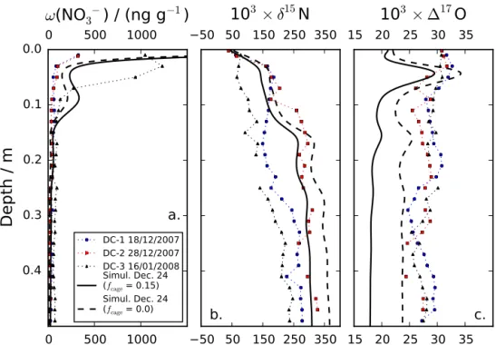
0.7 to 2.4 ‰) with an annual average of (1.4±0.6) ‰. Figure 6 shows the specific case of the simulated snow nitrate for the week around 24 December in the case of the DC realistic simulation. Simulated nitrate mass fractions decrease by more than 2 orders of magnitude in the top 15 cm andδ15N and117O values increase and decrease with depth from 40 ‰ to a mean background value above 290 ‰ and from 21 ‰ to a mean background value below 18 ‰ at around 20–3 cm depth, respectively. The simulated profiles are smooth and a small secondary peak can be observed in the mass fraction profile at around 9 cm depth, a depth which corresponds to 1 year of snow accumulation.

Table 6 gives the simulated nitrate mass fluxes and their isotopic composition in the case of the DC realis-tic simulation. The FA/FPI ratio for the DC-like simula-tion is 1.8 %, which means that a small fracsimula-tion of the pri-mary input flux of nitrate is archived below 1 m. The re-maining fraction (FE/FPI =1−FA/FPI=98.2 %) is ex-ported outside the atmospheric box. The photolytic, depo-sition and export fluxes show a peak whose timing follows the sunlit season (Fig. 4a). The annual photolytic flux is 32.1×10−6kgN m−2a−1and is compensated for by an an-nual deposition flux of 32.2×10−6kgN m−2a−1. Annually, the simulated FD and FP fluxes represent 4 times the primary input flux of nitrate (FD≈FP≈4×FPI). In the archived ni-trate, the simulated mass fraction, δ15N and 117O values are constant throughout the season: 23.0 ng g−1_{, 318 ‰ and}

17.8 ‰, respectively (Fig. 5, Table 6).

3.2.2 Simulation results across East Antarctica

Figure 7 shows the results for the TRANSITS simulations across East Antarctica in which only the snow accumula-tion rate is varied. The simulated 15N/14N apparent frac-tionation constants are low ((−46.1±2.2) ‰, n=4) for East Antarctic Plateau sites (A≤50 kg m−2_a−1_{; Erbland et}

al., 2013) and close to zero ((−10.3±9.0) ‰, n=3) for coastal sites (A≥200 kg m−2a−1). Also, simulated plateau sites feature an average17Eapp value, which is significantly

positive ((+1.0±0.3) ‰, Fig. 7b). The simulated archived flux (FA) and117O(FA) both decrease with increasing 1/A (Fig. 7e and d). Simulated δ15N(FA) values monotonically increase with increasing 1/A.

Figure 8 presents the same results in a different way. Panel a is a “modified Rayleigh plot” where ln(δ15N(FA) +1) is represented as a function of ln(FA) (which equals ln(ω(FA)×A))instead of ln(ω(FA)). In this representation, we observe that the simulated data fall on a line whose slope is−0.064. Figure 8b shows that 117O(FA) and δ15N(FA) (Fig. 8b) are negatively correlated.

3.3 Evaluation and discussion

In this section, we evaluate the model results in light of the observational constraints described above. In particular, we attempt to clearly state those observations which are well re-produced by the model and those which are not. In the sec-tions below, we also discuss the choice of the adjustment pa-rameters which were made to run TRANSITS.

3.3.1 Validation of the mass loss, diffusion and

15_N/14_{N fractionation process}

The nitrate mass loss is quantitatively represented in the TRANSITS model. Indeed, Fig. 6a shows that nitrate mass fractions decrease by a factor of 10 in the top 1 cm of the snowpack in agreement with observations. Also, the simu-lated archived nitrate mass fractions values are consistent with the observations (Fig. 5). This means that the nitrate mass fraction lost by photolysis (1−f )and calculated from the photolytic rate constant (J, Eq. 1) is quantitatively simu-lated by TRANSITS model runs.

Nitrate–δ15N isotopic profiles in snow also show that the

15_N/14_{N fractionation associated with nitrate photolysis is}

quantitatively represented within the uncertainties. Indeed, the DC realistic simulation reproduces well the depth pro-file ofδ15N in snow nitrate as observed in Fig. 6b, with sim-ulatedδ15N values as high as 150 ‰ at 1 cm depth. First, the simulated15N/14N apparent fractionation constants are consistent with the observations at Dome C (Fig. 5d) and for plateau sites (A≤50 kg m−2_a−1_{, Fig. 7a). This means that}

the absorption cross sections used for 14NO−₃ and 15NO−₃ (Berhanu et al., 2014a) and the variables used in the TUV-snow model (O3 column) allow a quantitative description

of the15N/14N fractionation constant associated with ni-trate photolysis (15εpho, Eq. 3). Secondly, the δ15N values

0

3

6

9

12

m

m

(N

O

−

)

/ (

mg

N

m

−

2

)

n = 4 3 5 3 2 5 4 4 4 1 6 10

a.

0

10

20

30

40

50

ω

(

FA

)

/ (

ng

NO

g

−

1

)

b.

50

100

150

200

δ

15

N

50c

m

(NO

)

×

10

3

c.

-90

-80

-70

-60

-50

-40

15

ǫ

p

×

10

3 ₁₅

_ǫ

pho

d.

240

260

280

300

320

δ

15

N(

FA

)

×

10

3

e.

05

10

15

20

25

30

∆

17

O

50c

m

(NO

3

−

)

×

10

3

f.

0.0

0.5

1.0

1.5

2.0

2.5

3.0

17

E

ap

p

×

10

3

g.

Jan Feb Mar Apr May Jun Jul Aug Sep Oct Nov Dec Jan Feb

05

10

15

20

25

30

∆

17

O(

FA

)

×

10

3

h.

Figure 5.Realistic simulation results for the snowpack and comparison to the observations at Dome C.(a)Nitrate mass in the top 5 cm (the

dashed curve represents the observed monthly values),(b)archived nitrate mass fractions,(c)δ15N of nitrate in the top 5 cm,(d)apparent and photolytic15εfractionation constants (in grey, the range±1σ ),(e)δ15N in the archived nitrate,(f)117O of nitrate in the top 5 cm,(g)

apparent17Efractionation constant (in grey, the range±1σ )and(h)117O in the archived nitrate. In each panel, the observed data from the three DC snow pits (Frey et al., 2009; Erbland et al., 2013) are represented by the same symbols as in Fig. 6.

the observations (from 275 to 300 ‰, Fig. 5f). This is fur-ther evidence that the nitrate mass fraction lost by photoly-sis (1−f )is quantitatively simulated by TRANSITS model runs. Indeed, using a quantum yield of 2.1×10−3at 246 K as in France et al. (2011) leads not only to an unrealistic FA/FPI ratio (71 %) andω(FA) value (917 ng g−1_{)but also}

to a very smallδ15N(FA) value (+20.3 ‰), which clearly

re-flects a weak recycling and an overestimate of primary nitrate trapped in snow. The adjusted photolytic quantum yield of 8=0.026 allows for computation of a consistent variation range ofδ15N in nitrate archived at depth. Given the choice of a modeled cage effect offcage=0.15, we obtain an