Development of an in-house tool for liquefaction assessment of soils

DEVELOPMENT OF AN IN-HOUSE TOOL FOR

LIQUEFACTION ASSESSMENT OF SOILS

BERNARDO JOSÉ ANDRADE PEREIRA CARVALHO DISSERTAÇÃO DE MESTRADO APRESENTADA

À FACULDADE DE ENGENHARIA DA UNIVERSIDADE DO PORTO EM ENGENHARIA CIVIL – ESPECIALIZAÇÃO EM GEOTECNIA

D

EVELOPMENT OF AN IN

-

HOUSE TOOL

FOR LIQUEFACTION ASSESSMENT OF

SOILS

B

J

A

P

C

Dissertação submetida para satisfação parcial dos requisitos do grau de MESTRE EM ENGENHARIA CIVIL —ESPECIALIZAÇÃO EM GEOTECNIA

Orientador: Professor Doutor António Milton Topa Gomes

Coorientador: Doutor Iain John Tromans Coorientador: Engenheira Manuela Daví

Tel. +351-22-508 1901 Fax +351-22-508 1446  [email protected]

Editado por

FACULDADE DE ENGENHARIA DA UNIVERSIDADE DO PORTO Rua Dr. Roberto Frias

4200-465 PORTO Portugal Tel. +351-22-508 1400 Fax +351-22-508 1440  [email protected]  http://www.fe.up.pt

Reproduções parciais deste documento serão autorizadas na condição que seja mencionado o Autor e feita referência a Mestrado Integrado em Engenharia Civil - 2015/2016 - Departamento de Engenharia Civil, Faculdade de Engenharia da Universidade do Porto, Porto, Portugal, 2016.

As opiniões e informações incluídas neste documento representam unicamente o ponto de vista do respetivo Autor, não podendo o Editor aceitar qualquer responsabilidade legal ou outra em relação a erros ou omissões que possam existir.

Este documento foi produzido a partir de versão eletrónica fornecida pelo respetivo Autor.

Aos meus Pais,

“One’s destination is never a place, but a new way of seeing things” Henry Miller

ACKNOWLEDGMENTS

Firstly I would like to express my thanks for this opportunity at CH2M and to the persons who made it possible. It was an incredible experience and it represents a remarkable period of my life, contributing to the development of my capabilities, allowing me to expand my knowledge and to get a closer look at the work developed within the engineering practice. My special gratitude goes then to the mentor of this agreement between the company and FEUP, Eng. João Fonte, who integrated me and made sure I was adapting not only to the company, but also to my life in London.

I would also like to acknowledge my gratefulness to my supervisors at CH2M. Eng. Manuela Daví, who from my first day at the company provided me the best conditions to develop a solid work and steered me in the right direction. Once again, my special gratitude for her availability and supervision, without whom it would not have been possible to accomplish the objectives set. Also to Dr. Iain Tromans, whose advice was indispensable for the development of my work. It was undoubtedly a privilege to have the possibility to work with such a great professional and an incredible team leader.

I would also like to acknowledge my thesis advisor at FEUP, Professor António Topa Gomes, whose virtual office had the door always open to any questions. I also thank him for his guidance during my Masters in Geotechnical Engineering, proving to be extremely professional and always maintaining a close relationship with his students.

I also want to express my gratitude to my colleague and friend Ana Rita, with whom I shared this experience abroad and whose support was vital during this period. My fingers are crossed for her and I am totally sure she will succeed in this new thrilling stage in her life.

I want to express my gratefulness to my friend Filipa, who even far away showed an incredible and indispensable support. I hope her to have a bright future as she deserves it and to be there to celebrate it with her.

To Diogo and Tiago, whose friendship was indeed one of the greatest gifts I had. I know for sure that we will keep improving it through great dinners and vacations.

To all my colleagues and friends at FEUP that accompanied me through the last five years, of which I underline Pinto, Zé, Francisca and Lili. It was a pleasure to share this ride with them and I wish them the best of lucks in their futures.

Last but not least, a very special thank you to my family, especially to my parents who provided me a great education but more importantly, values that I honour. Without their accompaniment, it would not have been possible to live this experience or to graduate.

ABSTRACT

An in-house soil liquefaction assessment tool based on CPT procedures is developed using Mathcad as platform. Three software packages are assessed by mutual comparison, namely CLiq (Geologismiki), LiquefyPro (CivilTech) and Settle3D _{(Rocscience). The aim of the developed in-house tool is to validate}

the software CLiq, as it is the only that embodies the same CPT-based liquefaction assessment procedure implemented on the tool. The validation is based on case histories selected from the New Zealand Geotechnical Database (NZGD), which provides an extensive archive of CPT data and post-earthquake information from the 2010-2011 Canterbury earthquake sequence. The seismic parameters as well as the post-earthquake information extracted are related to the MW 6.2, 2011 Christchurch earthquake, the

most damaging event in terms of liquefaction occurrence within the 2010-2011 Canterbury sequence. The three software packages are validated by comparing their calculated parameters against each other, using the Robertson and Wride (1998) liquefaction evaluation procedure, as it is one of the most established methods in earthquake engineering practice. The predicted liquefaction-induced settlements are also compared using the methods incorporated within LiquefyPro and CLiq, since Settle3D _{does not}

allow settlement estimation for CPT-based procedures (Tokimatsu and Seed, 1987; Ishihara and Yoshimine, 1992; Zhang et al., 2002 and Robertson and Shao, 2010).

Within the aim of this thesis, the tool has been developed to implement the latest and widely used method for liquefaction assessment in the engineering practice, i.e. Robertson (2009), an update of the Robertson and Wride (1998) procedure, as it was concluded through the literature review presented in chapter 2 and engineering practice in actual project in CH2M. A second part of the validation consists in plotting the parameters estimated by the tool and the software CLiq against each other using Robertson (2009). This study helps in identifying capabilities and limitations of the three commercially available software packages and highlights the benefits of having a custom-made in-house tool to assess soil liquefaction, flexible to adaptation and updates as new techniques become available.

RESUMO

No âmbito desta tese é desenvolvida uma ferramenta baseada em métodos CPT para avaliar o solo à liquefação. Três programas são avaliados através da comparação dos seus resultados, nomeadamente CLiq (Geologismiki), LiquefyPro (CivilTech) e Settle3D _{(Rocscience). O objetivo da ferramenta}

desenvolvida é o de validar o programa CLiq, uma vez que é o único dos três que incorpora o mesmo método CPT para avaliação do solo à liquefação que foi introduzido na ferramenta. A validação é baseada em casos históricos selecionados a partir da New Zealand Geotechnical Database (NZGD), que providencia um extenso arquivo de dados CPT e informação pós-sismo da sequência sísmica de Canterbury, 2010-2011. Os parâmetros sísmicos, assim como a informação pós-sismo são retirados do abalo sísmico de 2011 em Christchurch de magnitude 6.2, o evento que causou mais danos relacionados com a ocorrência de liquefação da sequência sísmica de Canterbury, 2010-2011.

A validação dos três programas consiste em comparar os parâmetros calculados entre eles, com recurso ao método de Robertson and Wride (1998) de avaliação em relação à liquefação, por ser um dos métodos mais utilizados pela comunidade de engenharia sísmica. Os assentamentos induzidos por liquefação estimados pelos programas são também comparados, usando os métodos incorporados no LiquefyPro e no CLiq, uma vez que o Settle3D _{não permite estimar assentamentos para análises baseadas em ensaios}

CPT (Tokimatsu and Seed, 1987; Ishihara and Yoshimine, 1992; Zhang et al., 2002 e Robertson and Shao, 2010).

No âmbito do objetivo da tese, a ferramenta é desenvolvida para incorporar o método mais recente e currentemente utilizado pela comunidade de engenharia sísimica em avaliações à liquefação, i.e. Robertson (2009), uma atualização do método de Robertson and Wride (1998), como foi concluido após a pesquisa bibliográfica apresentada no capítulo 2 e pela prática em projeto na CH2M. A segunda parte da validação consiste em representar gráficamente os parâmetros estimados pela ferramenta desenvolvida e pelo CLiq através do método de Robertson (2009).

Este estudo ajuda a identificar as capacidades e limitações dos três programas comerciais e realça os beneficios de possuir uma ferramenta interna para avaliar o solo em relação à liquefação, flexível para adaptações e atualizações que possam surgir com novas técnicas desenvolvidas.

GENERAL INDEX

ACKNOWLEDGMENTS ... I

ABSTRACT ... III

RESUMO ... V

1. INTRODUCTION ... 1

1.1. MOTIVATION AND GOALS ... 1

1.2. THESIS ORGANIZATION ... 3

2. LITERATURE REVIEW... 5

2.1. SOIL LIQUEFACTION ... 5

2.1.1.DEFINITION ... 5

2.1.2.EVALUATION OF SOIL LIQUEFACTION ... 6

2.1.2.1.Flow Liquefaction ... 6

2.1.2.1.Cyclic Softening ... 6

2.1.3.LIQUEFACTION SUSCEPTIBILITY ... 7

2.1.3.1.Compositional Criteria ... 7

2.1.3.2.Historical and Geological Criteria ... 8

2.1.3.3.State Parameter Criteria ... 9

2.1.4.INITIATION OF LIQUEFACTION ... 10

2.1.4.1.Characterization of Earthquake Loading ... 11

2.1.4.2.Characterization of Liquefaction Resistance ... 13

2.1.5.LIQUEFACTION EFFECTS... 15

2.1.5.1.Alteration of Ground Motion ... 16

2.1.5.2. Sand Boils ... 17

2.1.5.1.Settlement ... 17

2.2. CPTBASED LIQUEFACTION TRIGGERING PROCEDURES ... 17

2.2.1.DETERMINISTIC APPROACH ... 18

2.2.1.1.Robertson and Wride (1998) ... 18

2.2.1.2.Robertson (2009) ... 22

2.2.2.PROBABILISTIC APPROACH ... 25

2.2.2.2.Boulanger and Idriss (2014) ... 29

2.2.2.3.Ku et al. (2011) – Probabilistic version of Robertson and Wride (1998) ... 35

2.3. LIQUEFACTION POTENTIAL INDEX ... 36

2.4. CPTBASED LIQUEFACTION INDUCED GROUND SETTLEMENTS ESTIMATION ... 37

2.4.1.SATURATED SOILS SETTLEMENTS ... 37

2.4.1.1.Zhang et al. (2002) ... 37

2.4.1.2.Juang et al. (2013) ... 40

2.4.2.DRY SOILS SETTLEMENTS ... 42

2.5. DESIGN CODES APPROACH FOR LIQUEFACTION ASSESSMENT ... 44

2.5.1.AASHTOGUIDE FOR LRFDSEISMIC BRIDGE DESIGN ... 44

2.5.2.EUROCODE 8:DESIGN OF STRUCTURES FOR EARTHQUAKE RESISTANCE –PART 5:FOUNDATIONS, RETAINING STRUCTURES AND GEOTECHNICAL ASPECTS.BRITISH STANDARD ... 46

3. IMPLEMENTATION OF A CPT BASED MATHCAD

TOOL TO ASSESS LIQUEFACTION TRIGGERING ... 49

3.1. CAPABILITIES OF MATHCAD ... 49

3.2. DEVELOPMENT OF THE TOOL ... 49

3.2.1.CALCULATION SEQUENCE OF THE DEVELOPED TOOL ... 50

3.2.1.1.CPT Profile and Soil Parameters ... 51

3.2.1.2.Groundwater Depths ... 52

3.2.1.3.Seismic Parameters ... 53

3.2.1.4.CPT Values Correction ... 54

3.2.1.5.CRR7.5 ... 54

3.2.1.6.Magnitude Scaling Factor, MSF ... 55

3.2.1.7.CRR ... 55

3.2.1.8.CSR... 56

3.2.1.9.Factor of Safety, FS ... 56

3.2.1.10. Probability of Liquefaction, PL ... 57

3.2.1.11. Liquefaction Potential Index, LPI ... 58

3.2.1.12. Saturated Soil Settlements, Ss ... 59

3.2.1.13. Dry Soil Settlements, Sd ... 60

3.2.1.14. Probabilistic Settlements, PS ... 61

3.3. TOOL USER’S MANUAL ... 63

3.3.1.STARTING A NEW PROJECT AND DEFINING CALCULATION PARAMETERS AND PROCEDURES ... 63

3.3.2.PERFORMING THE CALCULATION ... 65

4. SELECTION OF CASE HISTORIES... 67

4.1. INTRODUCTION ... 67

4.2. CANTERBURY GEOLOGICAL CHARACTERIZATION ... 67

4.3. SELECTION OF CASE HISTORIES ... 69

4.3.1.NZGD-METHODOLOGY USED TO OBTAIN DATA VALUES... 70

4.3.1.1.Geotechnical Investigation Data ... 70

4.3.1.2.Liquefaction Interpreted from Aerial Photography ... 71

4.3.1.3.Vertical Ground Movements ... 72

4.3.1.4.Event Specific Groundwater Surface Elevations ... 72

4.3.1.5.Conditional PGA for Liquefaction Assessment ... 72

4.3.2.SELECTED CASE HISTORIES ... 73

4.3.2.1.Criteria Implemented ... 73

4.3.2.2.CPT-NBT-03 ... 77

4.3.2.3.CPT-KAN-26 ... 79

4.3.2.4.CPT-KAS-19 ... 80

5. VALIDATION OF SOFTWARE PRODUCTS ... 83

5.1. INTRODUCTION ... 83

5.2. LIQUEFYPRO ... 83

5.2.1.INPUT... 84

5.2.2.CAPABILITIES AND IMPLEMENTED METHODS ... 85

5.2.3.OUTPUT ... 86

5.3. SETTLE3D ... 87

5.3.1.INPUT... 87

5.3.2.CAPABILITIES AND IMPLEMENTED METHODS ... 88

5.3.3.OUTPUT ... 89

5.4. CLIQ ... 90

5.4.1.INPUT... 90

5.4.3.OUTPUT ... 92

5.5. COMPARISON OF SOFTWARE PRODUCTS ... 93

5.5.1.CPT-NBT-03 ... 95 5.5.1.1.Liquefaction Evaluation ... 95 5.5.1.2.Liquefaction-Induced Settlements ... 99 5.5.2.CPT-KAN-26 ... 102 5.5.2.1.Liquefaction Evaluation ... 102 5.5.2.2.Liquefaction-Induced Settlements ... 107 5.5.3.CPT-KAS-19 ... 109 5.5.3.1.Liquefaction Evaluation ... 110 5.5.3.2.Liquefaction-Induced Settlements ... 116 5.6. DISCUSSION ... 119 5.6.1.LIQUEFYPRO ... 120 5.6.2.SETTLE3D ... 121 5.6.3.CLIQ ... 122

6. VALIDATION OF THE DEVELOPED TOOL ... 125

6.1. INTRODUCTION ... 125

6.2.CHARACTERISTICS OF THE VALIDATION ... 125

6.3. COMPARISON OF THE PARAMETERS CALCULATED ... 126

6.3.1.LIQUEFACTION EVALUATION ... 126

6.3.2.LIQUEFACTION-INDUCED SETTLEMENTS ... 130

6.4. SENSITIVITY ANALYSIS ... 135

6.5. DISCUSSION ... 137

7. CONCLUSION ... 139

7.1. FINAL DISCUSSION ... 139

7.2. RECOMMENDATIONS FOR FURTHER DEVELOPMENTS ... 141

REFERENCES ... 143

FIGURES INDEX

Figure 1- Damage caused by liquefaction on buildings after the 1964 Niigata earthquake (Japan National Committee on Earthquake Engineering, 1968) ... 1 Figure 2- Sand boils evidencing liquefaction in the 2011 Christchurch earthquake at the Queen Elizabeth II Park (New Zealand Defence Force, 2011) ... 2 Figure 3- Scheme presented by Ishihara (1985) to explain liquefaction phenomena (modified after Matos Fernandes, 2006): a) before liquefaction occurred b) during liquefaction c) after liquefaction ... 6 Figure 4- Flowchart for evaluation of soil liquefaction (Robertson 1994) ... 7 Figure 5- Liquefaction susceptibility criteria (Bray and Sancio, 2006) ... 8 Figure 6-Relationship between epicentral distances of sites at which liquefaction was observed and the magnitude of the earthquake (Kamer, 1996 after Ambraseys, 1988) ... 9 Figure 7 - Definition of state parameter (Kramer, 1996) ... 10 Figure 8- Simplified method to estimate shear stresses induced by earthquake (adapted from Seed and Idriss, 1971 after Matos Fernandes, 2011) : a) soil column considered; b) propagation in depth of shear stresses considering a stiff or flexible soil mass; c) evolution in depth of the stress reduction factor, rd. ... 12 Figure 9- Correlation between the number of equivalent uniform stress cycles with the earthquake magnitude (Seed and Idriss 1975) ... 13 Figure 10- Relationship between CSR and N160 values for silty sands in M=7.5 earthquakes (Kramer, 1996 after Seed et al. 1975) ... 14 Figure 11- Potential effects of liquefaction on pile foundations. The strains that may develop in a liquefied layer can induce high bending moments in piles. (Kramer, 1996) ... 16 Figure 12- Ground oscillation (a) before and (b) after earthquake (Kramer, 1996) ... 16 Figure 13- Photo of sand boils formed after the 1989 Loma Prieta earthquake (J.C. Tinsley, 1989) ... 17 Figure 14- Normalized CPT soil behaviour chart type (Robertson, 1990) ... 20 Figure 15- Recommended grain characteristic correction to obtain clean sand equivalent CPT penetration resistance in sandy soils (Robertson and Wride, 1998) ... 21 Figure 16- Flowchart illustrating the calculation of the cyclic resistance ratio (Robertson and Wride, 1998) ... 22 Figure 17- CPT Soil Behaviour Type chart for liquefaction and cyclic softening (Robertson, 2009) .... 24 Figure 18- Flowchart illustrating the calculation of CRR (after Robertson, 2009) ... 25 Figure 19 - Contours of 5, 20, 50, 80 and 95% probability of liquefaction triggering as function of CSR* and qc,1,mod. Close circles are liquefied case histories and open circles are non-liquefied case histories (Moss et al., 2006) ... 28 Figure 20- Comparison of fines adjusted curves for PL=15% with previous curves (Moss et al., 2006) ... 29 Figure 21- Correlation between the overburden correction factor (CN) and the normalized vertical effective stress for different qc1Ncs values (Boulanger and Idriss, 2014) ... 31

Figure 22- MSF estimation based on qc1Ncs and earthquake magnitude values (Boulanger and Idriss,

2014) ... 33

Figure 23- Liquefaction triggering curves for probabilities of liquefaction of 15%, 50% and 85% for all sands (Boulanger and Idriss, 2014) ... 35

Figure 24- Correlation between Probability of Liquefaction and the Factor of Safety provided by Robertson and Wride (1998) (Ku et al., 2011)... 36

Figure 25- Estimation of postliquefaction volumetric strain of clean sands (modified from Ishihara and Yoshimine, 1992) ... 38

Figure 26- Correlation between postliquefaction volumetric strain and equivalent clean sand tip resistance for different factors of safety (Zhang et al., 2002) ... 39

Figure 27- Probabilistic liquefaction-induced settlement hazard curve for a case history at the Marina District after the 1989 Loma Prieta earthquake (Juang et al., 2013) ... 42

Figure 28 - Relationship between the stress ratio for M=7.5 earthquakes and N1(60) values for (A) - clean sands and (B) - silty sands with 1. 35% fines; 2. 15% fines; 3. <5% fines ... 47

Figure 29- Calculation sequence performed by the developed tool ... 51

Figure 30- Part of the input area within the Mathcad tool ... 53

Figure 31- Example of a CRR7.5 plot provided by the Mathcad tool. ... 55

Figure 32- Example of a plot of CRR alongside with CSR provided by the tool. ... 56

Figure 33- Example of a Factor of Safety plot provided by the tool. ... 57

Figure 34- Example of the PL expression and plot as presented in the Mathcad tool. ... 58

Figure 35- Example of the provided LPI plot within the tool. ... 59

Figure 36- Example of the provided plot of Ss for a specific case. ... 60

Figure 37- Example of the settlement of dry soils as provided by the Mathcad tool. ... 61

Figure 38- Example of the plot presenting PS within the tool. ... 62

Figure 39- Procedure to input the data and define the parameters required by the tool for a liquefaction assessment. ... 64

Figure 40- Parameters estimated by the tool in the course of a liquefaction evaluation. ... 65

Figure 41- Parameters estimated by the tool in the course of a settlement estimation. ... 66

Figure 42- Geological features of Canterbury area. Christchurch location is highlighted by a yellow square. (Modified after Browne et al., 2012. Modified after Field & Browne, 1989 Wood et al., 1989, Cox & Barrell, 2007 and Forsyth et al., 2008) ... 68

Figure 43- Cross section of the Quaternary deposits underlying Christchurch (Taylor et al., 2012 after Brown and Weeber, 1992) ... 68

Figure 44- Soil texture of Christchurch city area. Christchurch city area is highlighted by a black star. (GNS Science report after Environment Canterbury pers. comm.) ... 69

Figure 45- Types of field tests available in Christchurch area. (New Zealand Geotechnical Database (2016) "Geotechnical Investigation Data", Map Layer CGD0010, retrieved 15/06/2016 from https://canterburygeotechnicaldatabase.projectorbit.com/) ... 71

Figure 46- Water table elevations based on dip measurements. (Canterbury Geotechnical Database (2014) "Event Specific Groundwater Surface Elevations", Map Layer CGD0800 – 12 June 2014,

retrieved 15/06/2016 from https://canterburygeotechnicaldatabase.projectorbit.com/) ... 72

Figure 47- Map layer with the strong motion station network available in the Christchurch area (Canterbury Geotechnical Database (2015) "Conditional PGA for Liquefaction Assessment", Map Layer CGD5110 – 30 June 2015, retrieved 15/06/2016 from https://canterburygeotechnicaldatabase.projectorbit.com/) ... 73

Figure 48- Map layer of liquefaction interpreted from aerial photographs, with each CPT selected represented (Canterbury Geotechnical Database (2013) "Liquefaction Interpreted from Aerial Photography", Map Layer CGD0200 - 11 Feb 2013, retrieved 15/06/2016 from https://canterburygeotechnicaldatabase.projectorbit.com/) ... 75

Figure 49- Map layer available in NZGD with the median PGA contours for the Christchurch earthquake event. The red dots represent the ground motion stations and the selected CPT’s are presented as well. (Canterbury Geotechnical Database (2015) "Conditional PGA for Liquefaction Assessment", Map Layer CGD5110 – 30 June 2015, retrieved 15/06/2016 from https://canterburygeotechnicaldatabase.projectorbit.com/) ... 76

Figure 50- Vertical ground movements for each CPT location provided by NZGD (Canterbury Geotechnical Database (2012) "Vertical Ground Surface Movements", Map Layer CGD0600 - 23 July 2012, retrieved 15/06/2016 from https://canterburygeotechnicaldatabase.projectorbit.com/) ... 76

Figure 51- Distance between CPT-NBT-03 location and the borehole used to perform the soil profile, represented by the line in yellow. (New Zealand Geotechnical Database (2016) "Geotechnical Investigation Data", Map Layer CGD0010, retrieved 15/06/2016 from https://canterburygeotechnicaldatabase.projectorbit.com/) ... 77

Figure 52- Plot of Fr and Qtn compared with soil profile of CPT-NBT-03 ... 78

Figure 53- Distance between CPT-KAN-26 location and the borehole used in the performance of the soil profile, represented by the line in yellow. (New Zealand Geotechnical Database (2016) "Geotechnical Investigation Data", Map Layer CGD0010, retrieved 15/06/2016 from https://canterburygeotechnicaldatabase.projectorbit.com/) ... 79

Figure 54- Plot of Fr and Qtn compared with the soil stratification ... 80

Figure 55- Distance between CPT-KAS-19 and the borehole selected to perform the soil profile, represented by the line in yellow. (New Zealand Geotechnical Database (2016) "Geotechnical Investigation Data", Map Layer CGD0010, retrieved 15/06/2016 from https://canterburygeotechnicaldatabase.projectorbit.com/) ... 81

Figure 56-Plot of Fr and Qtn compared with the soil profile of CPT-KAS-19 ... 82

Figure 57- Example of CPT data input in LiquefyPro ... 84

Figure 58- Selection of calculation methods in LiquefyPro ... 85

Figure 59- Example of an output graph report in LiquefyPro ... 86

Figure 60- Spreadsheet provided by Settle3D _{to insert the CPT data ... 88}

Figure 61- Example of an output provided by Settle3D _{... 90}

Figure 63- Example of the graphical output provided by CLiq ... 93

Figure 64- Comparison of IC values estimated in CLiq and LiquefyPro ... 96

Figure 65- Comparison of values estimated by the three software products for CPT-NBT-03: a) CSR/CRR; b) FS ... 98

Figure 66- Comparison of settlements estimated by LiquefyPro and CLiq for CPT-NBT-03: a) saturated soils; b) dry soils. ... 100

Figure 67-Total Settlement estimated by LiquefyPro and CLiq for CPT-NBT-03... 101

Figure 68- Plot comparing IC values estimated by LiquefyPro and CLiq ... 103

Figure 69- Comparison of values estimated by LiquefyPro: a) IC; b) F and c) KC ... 104

Figure 70- Comparison of parameters estimated from three software products for CPT-KAN-26: a) CRR/CSR; b) FS. ... 106

Figure 71- Settlement estimated by LiquefyPro and CLiq for CPT-KAN-26: a) Saturated Soils; b) Dry Soils ... 108

Figure 72- Total Settlement estimated by LiquefyPro and CLiq for CPT-KAN-26 ... 109

Figure 73- IC estimated by LiquefyPro and CLiq for CPT-KAS-19 ... 111

Figure 74- Comparison of parameters estimated by LiquefyPro, CLiq and Settle3D_{: a) CRR and CSR; b)} FS ... 113

Figure 75- Comparison of parameters estimated by CLiq: a) IC; b) qc1Ncs; c) CRR ... 114

Figure 76- Comparison of parameters estimated by LiquefyPro: a) IC; b) qc1Ncs; c) CRR ... 115

Figure 77- Comparison of parameters estimated by Settle 3D: a) IC; b) CRR; c) FS. ... 116

Figure 78- Estimation of settlements after LiquefyPro and CLiq for CPT-KAS-19: a) saturated soils; b) dry soils ... 118

Figure 79- Total Settlement estimated by LiquefyPro and CLiq for CPT-KAS-19... 119

Figure 80- Comparison of parameters estimated from the developed tool and CLiq for CPT-NBT-03: a) IC; b) Qtn,cs. ... 127

Figure 81- Comparison between parameters estimated from CLiq and the developed Mathcad tool for CPT-NBT-03: a) CRR7.5; b) CSR ... 128

Figure 82- Comparison of parameters estimated by CLiq and Mathcad tool: a) FS; b) LPI; c) PL ... 130

Figure 83- Comparison of saturated soils settlement related parameters estimated by CLiq and Mathcad tool for CPT-NBT-03: a) εv; b) Ss ... 132

Figure 84- Comparison of dry soils settlement related parameters for CPT-NBT-03: a) εvol. ; b) Sd. .. 133

Figure 85- Comparison of the total settlement estimated by CLiq and the developed tool for CPT-NBT-03. ... 134

Figure 86- Results of sensitivity analysis performed to the Mathcad tool regarding the extension of the limit value for the CRR7.5-Qtn,cs relationship : a) Qtn,cs; b) FS ... 136

TABLES INDEX

Table 1- Comparison of Advantages and Disadvantages of Various Field Tests for Assessment of

Liquefaction Resistance, Youd et al. (2001) ... 15

Table 2-Characterization of liquefaction severity based on LPI values (after Iwasaki et al., 1982, and Luna and Frost, 1998) ... 37

Table 3- Statistical parameters obtained to characterize the model bias M (after Juang et al., 2013) . 41 Table 4- Partitions for Seismic Design Categories (AASHTO Guide Specifications for LRFD Seismic Bridge Design, 2009) ... 45

Table 5- Magnitude scaling factors proposed by Eurocode 8 - Part 5 ... 46

Table 6- Characteristics of the developed tool ... 63

Table 7- Criteria implemented to define liquefaction severity (after New Zealand Geotechnical Database) ... 71

Table 8- Criteria adopted in the selection of case histories ... 74

Table 9- Description of the selected case histories... 74

Table 10- Methodology implemented on the validation of the three software products ... 94

Table 11- Summary of LiquefyPro characteristics ... 121

Table 12- Summary of Settle3D characteristics ... 122

Table 13-Summary of CLiq characteristics ... 123

SYMBOLS,ACRONYMS AND ABBREVIATIONS

Latin Alphabet:

AASHTO- American Association of State Highway and Transportation Officials amax- maxi mum acceleration at ground surface

BPT- Becker Penetration Test c- Normalization exponent C0 – Fitting parameter for CRR7.5 CFC – Fitting parameter for FC

CN- Correction factor for overburden stress CQ- Correction factor for overburden stress CPT- Cone Penetration Test

CPTu- Piezocone Penetration Test CRR- Cyclic Resistance Ratio

CRR7.5- Cyclic Resistance Ratio for magnitude of 7.5 CSR- Cyclic Stress Ratio

CSR*_{- Equivalent uniform CSR for a magnitude of 7.5} Dr – Relative density

d- depth

DMT- Flat Dilatometer Test DWFM- Duration Weighting Factor e0- initial void ratio

ec- critical void ratio

ess- void ratio for the steady state line F- Normalized friction ratio from CPT Fr - Normalized friction ratio from CPT FC- Fines Content

FS- Factor of Safety fs- sleeve friction from CPT g- gravitational acceleration G0- Small strain shear modulus

GWT- Ground Water Table IC- Soil Behaviour Type Index

IND- Indicator of liquefaction occurrence K0 – In-Situ earth pressure coefficient Kα- Static shear stress reduction factor Kσ – Overburden stress correction factor KC- Fines correction factor

LFRD – Load and Resistance Factor Design LiDAR- Light Detection And Ranging LL- Liquid Limit

LPI- Liquefaction Potential Index M- Moment magnitude scale MW- Moment magnitude scale MSF- Magnitude Scaling Factor m- Stress exponent

NC - Equivalent number of cycles

(N1)60,cs – Normalized penetration resistance in clean sands for SPT n- Stress exponent

NZGD- New Zealand Geotechnical Database

NCEER- National Center for Earthquake Engineering Research pa- Reference pressure

PGA- Peak Ground Acceleration PI- Plasticity Index

PL – Probability of liquefaction

PS – Probability of exceeding a specific settlement Q- Normalized cone penetration resistance

Qtn- Normalized tip resistance correct for overburden stress from CPT Qtn,cs- Normalized clean sand tip resistance from CPT

qc- tip resistance from CPT

qc,1- Normalized tip resistance from CPT

qc,1,mod – Modified normalized tip resistance from CPT

qc1N,cs- Normalized clean sand tip resistance from CPT Rf - Friction ratio

rd- stress reduction factor S- Settlement

SD1 – Spectral acceleration coefficient at 1.0-sec. period Sd – Dry soil settlement

Ss – Saturated soils settlement St – Total settlement

SCPT- Seismic Cone Penetration Test SPT- Standard Penetration Test SSL- Steady State Line

USGS- United States Geological Survey Vs- Shear wave velocity

WTe – Earthquake water table WTi – In-situ water table wc- water content z- depth

Greek Alphabet:

Δqc – Fines adjustment factor Δz - Thickness of the soil layer εv- Vertical strain

εvol - Volumetric strain

εvol (15) - Volumetric strain equivalent to 15 cycles γ- shear stress

γcyc- cyclic shear stress γs- soil unit weight γw- water unit weight μ- Mean

σ- Standard deviation

σv- Total vertical stress

σv0- Total vertical in-situ stress σ’v- Effective vertical stress σ’v0- Effective vertical in-situ stress τav – Average cyclic shear stress τmax- Maximum shear stress

Φ – Standard normal cumulative distribution function Φ-1 _{– Inverse normal cumulative distribution function}

1

INTRODUCTION

1.1. MOTIVATION AND GOALS

Soil liquefaction is one of the great issues affecting foundations in sandy soils. The propensity of cohesionless soils to densify when submitted to ground shaking is well known, however when the water table is near the surface the hazard increases. When the soil is saturated, cyclic loading occurs rapidly and under undrained conditions, causing an increase in pore water pressure with the tendency of the soil to densify. If the magnitude of the cyclic loading reaches high values, the pore water pressure may even the soil’s total stress, causing the effective stress to reach a value of zero which decreases the soil stiffness and strength, and produces large deformations. After the earthquake, the pore water pressure excess tends to dissipate, causing a rearrangement of the soil’s particles and consequently producing settlement of the ground surface. Obviously, this phenomenon has catastrophic effects in structures founded upon soils that experience it, causing severe structural damage as it can be observed in Figure 1. Liquefaction may be also evidenced by the ejection of liquefied soil through cracks on the ground caused during the earthquake, defined as sand boils and noticed in Figure 2.

Figure 1- Damage caused by liquefaction on buildings after the 1964 Niigata earthquake (Japan National Committee on Earthquake Engineering, 1968)

Once it became an important topic of study, several methods to assess and analyse it were developed over time, based on laboratory or field testing. In chapter two of the current thesis, some of the proposed

methods based on field testing (CPT) are presented, from liquefaction evaluation to liquefaction-induced settlement estimation methods.

There is then a requirement for liquefaction assessment of soils within seismic design for structures by implementing these methods. However, it was found important by the engineering practice to develop an automated liquefaction assessment calculation based on some of the methods in the literature, which led to the formulation of several commercial software products.

Figure 2- Sand boils evidencing liquefaction in the 2011 Christchurch earthquake at the Queen Elizabeth II Park (New Zealand Defence Force, 2011)

Nonetheless, some of the software products used in engineering practice offer little transparency to the user, providing only the calculation results as output, which does not convey confidence and may not be acceptable in the scope of some projects. Emerged then the necessity of validating the commercial software products employed in seismic design, in order to better understand their procedures and the legitimacy of the calculations performed.

In the scope of this thesis is developed a tool, running on Mathcad and implementing some of the methods available in literature. Its aim is to validate some commercial software products, by comparing the results of a liquefaction analysis developed in both. The operation of the developed tool is presented in chapter three. The analyses performed are grounded in case histories selected from the New Zealand Geotechnical database (NZGD), since it provides quality information from the 2010-2011 Canterbury earthquake sequence.

It should be noted the importance of having an in-house tool that strictly follows the literature methods, flexible to adaptation and updates as new techniques become available, and capable of identifying the capabilities of the commercial software products.

1.2. THESIS ORGANIZATION

This dissertation can be divided into five main sections and one appendix.

Chapter two presents the state-of-the-art in which this thesis is grounded. A brief introduction to the liquefaction phenomenon is presented along with the methods available in the literature to evaluate it and to estimate associated settlements. It is discussed the types of liquefaction, the methods available to evaluate it and the effects of this phenomenon on the ground. CPT-based methods are emphasized, having been selected as the field testing technique of most interest for the curent research project. Liquefaction evaluation methods are divided in deterministic and probabilistic, while settlement estimations methods are separated into those for saturated soils and those for dry soils.

Chapter three presents the CPT-based in-house tool developed in Mathcad. A brief discussion of this software is made, by presenting its capabilities and functionalities that support the selection of Mathcad to be the platform in which the tool runs. The calculation sequence is also presented by describing, for each step, the methods implemented and discussed in chapter two, as well as the data required by the tool to run the analysis and the parameters provided after the calculation. Snapshots of the calculation spreadsheet are provided, including the input area and graphical output of calculated parameters, in order to better understand the tool’s operation. The full worksheet developed for the tool is presented in appendix.

In chapter four, the case histories selected to perform the assessment of three software products and the validation of the developed tool against one of them are presented, as well as the criteria implemented in their selection. Three case histories are selected from the New Zealand Geotechnical Database, created after the 2010-2011 Canterbury earthquake sequence in New Zealand. A geological characterization of the Canterbury region is provided, emphasizing the Christchurch area, since the case histories selected are within it. The data available in the NZGD is presented, as well as the methods adopted to obtain it. After the selection of the case histories, it is provided the stratification of each location based on boreholes nearby.

In chapter five is carried out a validation of three commercial software products: LiquefyPro, Settle3D

and CLiq. The three software products are assessed and characterized by describing their functionality and methods available to perform a liquefaction evaluation or a liquefaction-induced settlement estimation. The validation is based on the methods of the software products and it is achieved by evaluating each of the three case histories selected in chapter four and plotting the calculated parameters from each software against the others. The results of the liquefaction assessments are also compared with the post-earthquake information available in NZGD. A final discussion gathers the findings of the validation process and summarizes the characteristics and limitations observed for each software. Chapter six presents the validation of the developed tool against one of the three commercial software products, CLiq. The validation process is similar to the one implemented in chapter five with a liquefaction evaluation made of one of the case histories, plotting the results computed from the tool against the same parameters obtained by CLiq. A sensitivity analysis is also developed herein, in order to check the influence on the results of some modifications made to the literature procedures implemented in the tool and in CLiq. To conclude, the results of the validation and the sensitivity analysis are discussed, presenting an overview of the developed tool.

Chapter seven summarizes the work developed and the conclusions obtained after each validation. A proposal for further developments of the work realized is also presented in this chapter, considering the opportunities for enhancement of the tool and the process of validation, from the point of view of the author.

2

LITERATURE REVIEW

2.1. SOIL LIQUEFACTION

2.1.1.DEFINITION

Liquefaction is an important topic to study and to consider in the design of structures constructed upon saturated sandy soils, due to its devastating effects. Although Duton had already noticed liquefaction evidence in the 1886 Charleston earthquake, and Mogami and Kubo (1953) conceived the term liquefaction as the total loss of strength of vibrated sands, according to Scawthorn (2006), the process of studying the liquefaction phenomenon had only intensified after the Niigata and the Alaska earthquakes in 1964, where both earthquakes produced examples of liquefaction-induced damage, such as slope failures, bridge and building foundation failures and flotation of buried structures – Kramer (1996).

Terzaghi and Peck (1963) defined liquefaction as the sudden drop of shear strength under undrained conditions from the yield strength to the substantially smaller critical state strength. This loss of strength induces a behaviour in the soil similar to a liquid. When a saturated cohesionless soil is submitted to a rapid loading under undrained conditions, its tendency to densify will produce an increase in the excess pore water pressure, causing a decreasing of the effective stresses – Kramer (1996). Ishihara developed a scheme to better explain what happens in terms of stresses during the occurrence of liquefaction, presented in Figure 3.

As there is not an established and prevailing approach to assess the triggering of liquefaction phenomena in a soil, due to the several procedures and methods of analysis, it is still a controversial topic, the understanding of which has been improved after major earthquake events such as the Loma Prieta (1989), Kobe (1995), Kocaeli (1999) and more recently the Canterbury earthquake sequence (2010-2011) in New Zealand.

Liquefaction phenomena can be divided in two major groups: flow liquefaction and cyclic softening. Although this dissertation will only focus on liquefaction cases of cyclic softening, it will be made a brief distinction between both so it is clearer to understand what the soil is experiencing in each situation.

Figure 3- Scheme presented by Ishihara (1985) to explain liquefaction phenomena (modified after Matos Fernandes, 2006): a) before liquefaction occurred b) during liquefaction c) after liquefaction

2.1.2.EVALUATION OF SOIL LIQUEFACTION 2.1.2.1. Flow Liquefaction

Flow liquefaction applies to strain softening soils and it occurs when the static shear stress is greater than the shear stress of the soil in its liquefied state – Kramer (1996). It can be triggered by a loading either monotonic or cyclic in loose and cohesionless deposits, very sensitive clays and silt deposits. For soil failure to occur, a sufficient volume of material should strain soften, and the resulting failure can be a slide or a flow depending on the material characteristics and the ground geometry – Robertson (2004). Although it is not very frequent to perceive an example of a failure due to flow liquefaction, when it happens the results are catastrophic as it was exemplified in the Aberfan flow slide – (Bishop, 1973), Zeeland sub-marine flow slides – (Koppejan et al., 1948) and the Sheffield and the Lower San Fernando dams.

2.1.2.1. Cyclic Softening

Cyclic softening can occur in saturated cohesionless soils with a strain hardening behaviour and it is characterized by a decreasing of the effective stresses in the soil due to an undrained cyclic loading. Cyclic softening may also be divided into two groups depending on the reversal of the shear stress. If it occurs, the soil experiences cyclic liquefaction, otherwise the phenomenon is called cyclic mobility. For shear reversal to occur, ground conditions must be level or gently sloping – Robertson and Wride (1998). If it occurs, the effective stress can reach a value of zero, causing a decrease in the soil stiffness and producing large deformations. The magnitude of the deformations depends on the density of the soil, the magnitude and duration of the cyclic loading and the extent to which shear stress reversal occurs (Robertson and Wride, 1998).

If there is no shear stress reversal and the cyclic loading is moderate, the effective stress barely drops to a value of zero, causing smaller deformations than cyclic liquefaction.

Robertson (1994) produced a flowchart evaluating liquefaction and characterizing its different types, as shown by Figure 4.

Figure 4- Flowchart for evaluation of soil liquefaction (Robertson 1994)

2.1.3.LIQUEFACTION SUSCEPTIBILITY

The first step in a liquefaction evaluation is the assessment of the susceptibility of a soil to liquefaction, since not all soils are potentially liquefiable. Liquefaction susceptibility can be evaluated through several criteria, presented below.

2.1.3.1. Compositional Criteria

As the aim of this project is to develop a tool to assess liquefaction linked to earthquake events, only cyclic liquefaction will be evaluated. The first step to evaluate cyclic liquefaction in level ground sites is to evaluate the soil susceptibility to this phenomenon. The Guide to Cone Penetration Testing for Geotechnical Engineering – Robertson and Cabal (2015), suggests that the susceptibility to cyclic liquefaction should be evaluated based on the plasticity index (PI), the liquid limit (LL) and the natural water content (wc) of a soil. The criteria followed by this guide was proposed by Bray and Sancio (2006),

and is presented in Figure 5.

It also should be considered the level of risk of each project before deciding whether a soil is susceptible or not. If a project has low risk, it should be assumed that a soil is susceptible to cyclic liquefaction based on the Bray and Sancio (2006) criteria, unless previous local experience shows otherwise – Robertson and Cabal (2015). If the risk of the project is high, it should be assumed that the soil is susceptible to liquefaction or high quality samples should be obtained and properly tested on laboratory.

If a soil is considered susceptible to cyclic liquefaction, the next step in liquefaction evaluation should be taken. In other words, it should be evaluated the triggering of cyclic liquefaction, presented hereafter.

Figure 5- Liquefaction susceptibility criteria (Bray and Sancio, 2006)

2.1.3.2. Historical and Geological Criteria

An important source of information in the evaluation of the susceptibility of a soil to liquefaction comes from historical data on previous earthquakes that caused liquefaction. Post-earthquake field investigations have shown that liquefaction often occurs at the same location if soil and groundwater conditions have remained unchanged – Youd (1984). Based on these investigations, Ambraseys (1988) compiled data from case histories to propose a relationship between the epicentral distance of sites at which liquefaction was observed and the magnitude of the earthquakes that produced liquefaction. This relationship is presented in Figure 6.

The geological criteria to assess the susceptibility of a soil to liquefaction is based on the depositional and hydrological environment, as well as the age of the deposit – Kramer (1996). Soils that are sorted into uniform grain size distributions and deposited in loose states have a high liquefaction potential. The water level has also great influence in liquefaction susceptibility, since liquefaction only occurs in saturated soils, causing fluvial and estuarine deposits to have high liquefaction potential. The susceptibility of older soils to liquefaction is lower than newer deposits – Kramer (1996).

Figure 6-Relationship between epicentral distances of sites at which liquefaction was observed and the magnitude of the earthquake (Kamer, 1996 after Ambraseys, 1988)

2.1.3.3. State Parameter Criteria

As mentioned previously, the base of liquefaction triggering is the generation of excess pore pressures when the soil is submitted to a cyclic loading. Since the tendency to generate pore pressure of a soil is influenced by its initial state, defined by density and initial stress conditions – Kramer (1996), liquefaction susceptibility can be evaluated through state criteria, as the state parameter.

To understand the concept of state parameter, it is necessary to discuss the concept of steady state of deformation, defined by Castro and Poulos (1977). Based in several stress-controlled undrained triaxial tests, the steady state of deformation was defined as the state in which the soil flowed continuously under constant shear stress and constant effective confining pressure at constant volume and velocity – Kramer (1996). The spatial distribution of the points that correlate the void ratio with the effective confining pressure of the soil in the steady state of deformation is defined as the steady-state line (SSL). The correlation between the state parameter and the steady state line is presented on Figure 7.

The state parameter represents the proximity of the soil’s initial state to the steady state line, and was defined by Been and Jeffries (1985) as:

c

e

e







Where e0 is the initial void ratio and ec, also represented as ess, is the void ratio of the steady-state line

The SSL has been proved to be useful identifying the susceptibility of a soil to flow liquefaction, since it can only occur in soils with positive values of the state parameter, in other words, soils with an initial void ratio higher than the critical, defined as soils with contractive behaviour. On the other hand, cyclic softening can occur in soils with contractive or dilative behaviour, with the initial void ratio lower than the critical. Given that, the state criteria does not represent a useful criteria in cyclic liquefaction evaluation.

Figure 7 - Definition of state parameter (Kramer, 1996)

2.1.4.INITIATION OF LIQUEFACTION

There are several approaches to evaluate the potential for initiation of liquefaction, the most common to use in geotechnical engineering practice are the cyclic stress and the cyclic strain approaches. The work reported on this thesis will be only based on the cyclic stress approach, once it may only require in-situ tests for the characterization of the liquefaction resistance.

To evaluate the initiation of liquefaction, this approach expresses the earthquake-induced loading in terms of cyclic shear stresses, and compares it with the liquefaction resistance of the soil, also expressed in terms of cyclic shear stress. At locations where the loading exceeds the resistance, liquefaction is expected to occur – Kramer (1996).

Seed and Idriss (1971) proposed a simplified procedure to evaluate the susceptibility of a soil to liquefaction, consisting on comparing the soil resistance with the cyclic loading by the means of a factor of safety against liquefaction. This parameter is defined by equation (2) and is estimated for each depth where soil resistance and earthquake loading are characterized.

CSR CRR

Where CRR is the cyclic resistance ratio and CSR the cyclic stress ratio. Both parameters will be presented further ahead. For depths where CSR is greater than CRR (FS < 1), it is considered the soil layer to be liquefiable, otherwise it is assumed that liquefaction will not occur.

2.1.4.1. Characterization of Earthquake Loading

To express the seismic loading in terms of cyclic shear stress, it can be made a ground response analysis or use a simplified approach – Kramer (1996). In this thesis it will be used the simplified approach developed by Seed and Idriss (1971) and presented in Figure 8. The following procedure for the estimation of the cyclic shear stress was extracted from Matos Fernandes (2011):

Consider a soil column with level ground conditions and height equal to z, submitted to horizontal accelerations. When they reach their maximum value at the surface, the peak ground acceleration (PGA), is installed in the bottom of the considered soil column a shear stress defined by:

0 max max

)

(

g

a









As the soil column is not stiff, the shear stress installed is smaller than the defined by the equation (3), and it can be obtained by introducing a stress reduction factor rd:

d v d r g a    0 max max) (





There are several approaches to define the stress reduction factor, in this thesis it will be assumed a set of expressions proposed by Liao and Whitman (1986), equations (5) and (6), Robertson and Wride (1997), equation (7), and William F. Marcuson in an oral communication, equation (8) – Youd and Idriss (1997). The expressions proposed by Liao and Whitman (1986) were recommended in the 1997 National Centre for Earthquake Engineering Research (NCEER) workshop and Youd et al. (2001):

9.15m z if 00765 . 0 1    z r_d 9.15m z 23m if 0267 . 0 174 . 1      z r_d 23m z 30m if 008 . 0 744 . 0      z r_d 30m z if 5 . 0   d r (5) (6) (7) (8)

These expressions provide a mean of a wide range of possible rd, and the range increases with depth –

Golesorkhi (1989), once there is a considerable variability in the soil’s flexibility at field sites. However, the participants of the workshop agreed that these expressions are suitable for use in engineering practice – Youd et al. (2001).

As the amplitude of an earthquake cyclic loading is quite odd, the shear stress will vary, so the assumption of a peak ground acceleration to characterize the seismic loading is not the more accurate. Seed and Idriss (1971) defined a uniform and equivalent cyclic loading with constant frequency and amplitude, with an amplitude equal to 65% of the maximum earthquake amplitude. The uniform cyclic shear stress is defined by:

d v cyc

r

g

a









₀

_.

₆₅





Figure 8- Simplified method to estimate shear stresses induced by earthquake (adapted from Seed and Idriss, 1971 after Matos Fernandes, 2011) : a) soil column considered; b) propagation in depth of shear stresses

considering a stiff or flexible soil mass; c) evolution in depth of the stress reduction factor, rd.

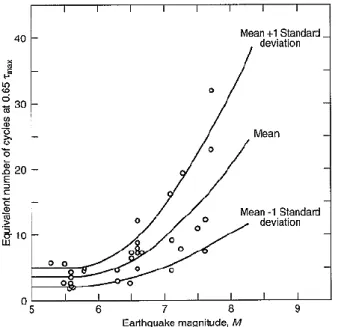
Regardless of whether a detailed ground response analysis or the simplified procedure is used, the earthquake-induced loading is characterized by a level of uniform cyclic shear stress applied for an equivalent number of cycles – Kramer (1996). The equivalent number of cycles depends on the earthquake magnitude, and the correlation between them was proposed by Seed et al. (1975) and presented on Figure 9

Maximum shear stress

De

pth

Figure 9- Correlation between the number of equivalent uniform stress cycles with the earthquake magnitude (Seed and Idriss 1975)

Dividing both members of the equation (9) by the initial effective overburden pressure to normalize the cyclic stress, it is obtained the cyclic stress ratio, CSR:

d v v v cyc

r

g

a

CSR











'

65

.

0

'









2.1.4.2. Characterization of Liquefaction Resistance

Resistance to cyclic loading is usually represented in terms of a cyclic stress ratio that causes cyclic liquefaction – Robertson and Wride (1998). To denote this ratio, different authors gave it different symbols but, as they used the symbol CSR with or without a subscript to signify liquefaction resistance, it generated some sort of confusion. So, in the workshop of the NCEER, Robertson and Wride proposed the term cyclic resistance ratio (CRR) to denote the liquefaction resistance – Youd and Idriss (1997). Cyclic resistance can be obtained both by laboratory testing and by field testing. Laboratory test consist in submitting soil samples to cyclic loading by means of cyclic triaxial, cyclic simple shear or cyclic torsional tests – Robertson and Wride (1998). For cyclic simple shear test, the CRR is taken as the ratio of the cyclic shear stress to cause liquefaction to the initial vertical effective stress. In the cyclic triaxial test, CRR is taken as the ratio of the maximum cyclic shear stress to the initial effective confining pressure – Kramer (1996). Liquefaction failure in a laboratory test is defined as the point at which the soil sample achieves a strain level of 5% for axial strain amplitude in a cyclic triaxial test – Robertson and Wride (1998). Although laboratory testing was the basis of the early works related with cyclic resistance, there are several issues that hamper its broader use in evaluating the CRR. The in-situ stress state is very difficult to reply on laboratory and the samples are easily disturbed during the sampling, which destroy the effects of the depositional and historical environment of a soil deposit that influence liquefaction resistance – Kramer (1996). A solution to surpass these limitations is ground freezing, used

to obtain undisturbed samples of cohesionless soil, but the implementation of this procedure is usually costly, so it is only adopted in high-risk projects, where laboratory tests are necessary.

An alternative to estimate the liquefaction resistance of a soil is through liquefaction case histories and soil parameters measured by field tests, and due to the costs and the difficulties associated with recovering good quality and undisturbed samples to use in laboratory tests, field tests are the dominant approach in engineering practice for evaluating liquefaction potential. – Juang et al. (2013)

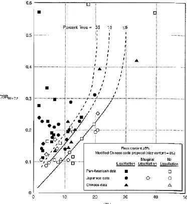
The first approaches were based on measured standard penetration test (SPT) parameters, plotted with the cyclic stress ratio that characterized the earthquake loading. The plotted points were distinguished whether liquefaction was observed or not, and a conservative boundary was drawn dividing the combinations that have or have not produced liquefaction in the past earthquakes – Kramer (1996). The observance of liquefaction cases is proven by the appearance of sand ejected through cracks and forming sand boils at ground surface. One of the first studies based on SPT was developed by Seed et al. (1975) plotting the cyclic stress ratio for an earthquake magnitude of 7.5 versus the blow count, presented in Figure 10.

Figure 10- Relationship between CSR and N160 values for silty sands in M=7.5 earthquakes (Kramer, 1996 after Seed et al. 1975)

The development of studies following this procedure and the introduction of new case histories, allowed the development of methodologies considering the fine content (Seed et al. 1985) and new approaches based on cone penetration test (CPT) results – Matos Fernandes (2011). Among the in-situ tests, CPT is the preferred tool for liquefaction evaluation, due to its repeatability, accuracy and the capacity of providing continuous profiling of the soil throughout the measured parameters, cone tip resistance (qc)

There are several more examples of field tests that can be used on the liquefaction assessment and that were object of research through the years, such as the Becker penetration test (BPT), the shear wave velocity measurement (VS) and the flat dilatometer test (DMT). The advantages and disadvantages of

some methods available for liquefaction assessment based on field tests were gathered by Youd and Idriss (2001) and presented on Table 1.

Table 1- Comparison of Advantages and Disadvantages of Various Field Tests for Assessment of Liquefaction Resistance, Youd et al. (2001)

In this thesis, the procedure to be followed on liquefaction assessment is the use of field tests to characterize liquefaction resistance of a soil, more specifically the CPT, since it provides good outcome and it is widely implemented. Within the CPT based procedures, there are several methods to assess liquefaction triggering, from deterministic approaches that express liquefaction potential in terms of a factor of safety, to probabilistic approaches that consider the uncertainties inherent to the parameters and express the liquefaction potential in terms of the probability of liquefaction – Juang et al. (2013). Those different methods will be presented and detailed hereafter along with their approaches to characterize the cyclic resistance of the soil.

The CRR is typically taken at about 15 cycles of uniform loading to represent an equivalent earthquake loading of magnitude, M, equal to 7.5, i.e., CRR7.5 – Robertson and Wride (1998). To obtain the cyclic

resistance for the design earthquake loading, the CRR7.5 provided from the CPT procedures should be

affected by a factor that accounts for the duration effects. The magnitude scaling factor, MSF, account for how the characteristics of the irregular cyclic loading produced by different magnitude earthquakes affect the potential for triggering of liquefaction – Boulanger and Idriss (2014). Each procedure to evaluate liquefaction triggering has a specific recommendation for MSF and they will be presented herein this thesis, in section 2.2.

The CRR for the design earthquake magnitude comes as:

MSF

CRR

CRR





2.1.5.LIQUEFACTION EFFECTS

As it was mentioned previously, liquefaction causes devastating damages on structures, sometimes more severe than the earthquake motion. These damages are due to the effects that a liquefied soil layer has on building foundations, on the surface, or even on the ground motion.

The effects of liquefaction provide evidence that a soil layer beneath the surface has liquefied, and are the base of case histories used by geotechnical earthquake engineering for progressing on this area.

2.1.5.1. Alteration of Ground Motion

The alteration of the ground motion is one effect of cyclic liquefaction that may cause damages on pile foundations and on the ground oscillation. The development of excess pore pressures during an earthquake will decrease the soil stiffness to values that can affect the transmission of the bedrock motion to the ground surface. Also, the occurrence of liquefaction beneath a level ground surface can decouple the liquefied soils from the surficial soils and produce transient ground oscillations – Kramer (1996). The soils at the surface may crack, causing liquefied soils to emerge and developing sand boils. Ground oscillation was the cause of the ground movements that fractured the pavements of the Marina District of San Francisco during the Loma Prieta earthquake in 1989. – Youd (1993). Figure 11 and Figure 12 represent the damage that the alteration of ground surface can induce.

Figure 11- Potential effects of liquefaction on pile foundations. The strains that may develop in a liquefied layer can induce high bending moments in piles. (Kramer, 1996)

Figure 12- Ground oscillation (a) before and (b) after earthquake (Kramer, 1996)

2.1.5.2. Sand Boils

The excess pore pressures developed during the earthquake motion tend to dissipate by an upward flow of pore water, producing forces on soil particles in the same direction. These forces can loosen the upper portion of the deposit and leave it in a state susceptible to liquefaction in a future earthquake event – Youd (1984). If the hydraulic gradient driving the flow reaches a critical value, the vertical effective stress will drop to zero and the soil will be in quick condition – Kramer (1996). The soil particles may be carried upwards by the water movement and be ejected at the surface through localized cracks, forming sand boils. The development of sand boils depends on the characteristics of the liquefied soil layer and the soil layer above, and on the magnitude of the excess pore pressure – Kramer (1996). Sand boils do not produce any damage but are a proper evidence of liquefaction, as it can be noticed in Figure 13

Figure 13- Photo of sand boils formed after the 1989 Loma Prieta earthquake (J.C. Tinsley, 1989)

2.1.5.1. Settlement

Cohesionless soils tend to densify when submitted to an earthquake loading, causing settlements on the ground surface. It can be divided in dry soils settlements, that are usually fast, and in saturated soils settlements, that take longer to occur depending on the time that excess pore pressures take to dissipate. As settlement causes more damage on structures and lifelines than other liquefaction effects, it will be object of further studies on subsequent chapters.

2.2. CPTBASED LIQUEFACTION TRIGGERING PROCEDURES

Due to its repeatability, accuracy and the capacity of providing continuous profiling of the soil throughout the measured parameters, cone tip resistance (qc) and sleeve friction (fs) – Juang et al. (2013),

the CPT is the preferred in-situ test to be the basis of a liquefaction assessment. The CPT-based procedures present their recommendations to estimate CRR7.5 and MSF. Seed and Idriss (1971)

recommendation to estimate CSR is considered accurate, so it is recommended by all presented methods. However, some may introduce new procedures to estimate rd, rather than the suggested by NCEER.

From the several CPT based procedures in the literature, only five will be presented in this chapter, divided into deterministic and probabilistic approaches.

2.2.1.DETERMINISTIC APPROACH

The deterministic approaches to determine the liquefaction potential of a soil give as an output, the factor of safety (FS) against liquefaction triggering. The FS correlates the seismic loading with the soils resistance to cyclic loading through a ratio between the CRRM and the CSR. For the depths in which the

FS is lower than 1 cyclic loading exceeds cyclic resistance, so liquefaction is expected.

The deterministic approaches to be followed in this report are the Robertson and Wride (1998) and the Robertson (2009). The latter can be considered as an update of Robertson and Wride (1998), but this will be analysed in more detail further ahead.

2.2.1.1. Robertson and Wride (1998)

This method suggests the Seed and Idriss (1971) approach, detailed in the subchapter 2.1.4.1. and defined by the equation (10) to estimate the CSR.

The authors suggest the use of CPT to estimate the CRR, since it provides great repeatability and a more continuous profile than the SPT – Robertson and Wride (1998). The output of a CPT test is the cone tip resistance (qc) and the sleeve friction (fs), and these values alongside with the total vertical in-situ stress

(σv0) and the effective vertical in-situ stress (σ’v0) are the basis for the CRR calculation.

The CRR7.5 expressions proposed by Robertson and Wride (1998) are based on the equivalent clean

sand normalized CPT penetration resistance (qc1N,cs), and they are defined by:

60 1 q 50 if 0.08 1000 93 _c1N,cs 3 , 1 5 . 7 _            qc N cs CRR 50 q if 0.05 1000 833 . 0 _c1N,cs 3 , 1 5 . 7            qc N cs CRR (12) (13)

To obtain the qc1n,cs it must be made a normalization and a correction for overburden stress, and also it

must be implemented a correction factor that accounts for the grain characteristics of the soil:

N c C cs N c K q q _{1 ,}   ₁ (14)

Where KC is the grain characteristics correction factor, which will be presented further ahead, and qc1N

2 1 2 1 a c Q a c N c P q C P q q _        (15)

Where CQ, defined in equation (16), is the correction for overburden stress and Pa2 is the reference

pressure that must be in the same unit as qc – Robertson and Wride (1998).

n v a Q P C _       0 '  (16)

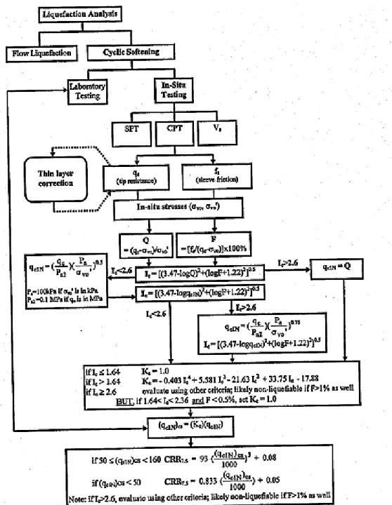
To establish a correction factor for the grain characteristics of the soil, it is necessary to estimate grain characteristics such as apparent fines content of the soil, once the correlations proposed for the CRR are very sensitive to the plasticity of the fines within the sand – Robertson and Wride (1998). The grain characteristics can be estimated from CPT results, by using soil behaviour charts. This method uses the normalized CPT soil behaviour type chart, proposed by Robertson (1990) and presented here in Figure 14, to obtain the soil behaviour type index (IC):



 



Where Q is the normalized CPT penetration resistance and F is the normalized friction ratio:

n v a a v c P P q Q _               0 2 0 '





%

100



















q

f

F



The soil behaviour type chart proposed by Robertson (1990) uses a normalized cone penetration resistance (Q) based on a stress exponent of n = 1.0, whereas the expressions proposed by Robertson and Wride (1998) to estimate CRR (equations (12) and (13)) are based on a normalized cone penetration resistance, qc1N, that uses a stress exponent n = 0.5 (equations (15) and (16)).

The stress exponent is complex to obtain, and Olsen and Malone (1988) suggested that it varies from 0.5 in sands to 1.0 in clays. The approach followed by Robertson and Wride (1998) begins by assigning a stress exponent equals to 1.0 to calculate Q and, therefore, an initial value of IC. If IC > 2.6, it should

be assumed that qc1N = Q. However, if IC ≤ 2.6, the exponent to calculate Q should be assumed as 0.5

and IC should be recalculated based on qc1N and F. If the recalculated IC remains less than 2.6, it should

be used the qc1N based on the stress exponent of 0.5 to estimate CRR, otherwise, a stress exponent of