Evolution, Ageing and Speciation:
Monte Carlo Simulations of Biological Systems
S. Moss de Oliveira
Instituto de F´ısica, Universidade Federal Fluminense Av. Litorˆanea s/n, Boa Viagem, Niter´oi, Brasil 24210-340
Received on 10 May, 2004
We present a complete description of the Penna bit-string model for biological ageing and how it has been modified, along the last 10 years, to simulate and better understand many different evolutionary phenomena. Particularly, we show how a phenotype was included into the model in order to study speciation and correlated problems.
1
Introduction
According to Luca Peliti [1], models to explain the origins of life and its evolution can be divided in three groups: i) Models for microevolution - individuals belong to the same species or to closed ones. Interaction among individ-uals is generally introduced through some global competi-tion mechanism; ii) Models for coevolucompeti-tion - two or more species interact strongly in such a way that the survival of one species depends on the survival of the other; iii) Models for macroevolution - also called large-scale models for evo-lution. They deal with all alive species at the same time, but with no particular interacting mechanism between them.
One of the pioneer models for microevolution was pro-posed by M. Eigen [2] as an attempt to explain the origins of life in Earth. It describes the dynamics of biological macro-molecules (that can replicate) under the influence of selec-tion and mutaselec-tion mechanisms. The macromolecules can be represented by bit-strings of zeroes and ones, each one with a given replication rate. Its main results are: without competition there is segregation among the macromolecules and those that present a replication rate higher than its death rate increase exponentially, while the others disappear. If a global competition mechanism is introduced (the total num-ber of macromolecules is forced to stay constant) then se-lection becomes active and only the macromolecule species with the maximum replication rate or fitness, called the mas-ter sequence, survives. When mutations are then included, different quasi-species coevolve in a fitness landscape where the initially best fitted master sequence occupies now one of the possible maxima of this landscape, surrounded by the other quasi-species. When the mutation rate surpasses a given threshold, however, selection disappears and all se-quences become equally probable. The main conclusion ob-tained from this simple model is that without errors (muta-tions) or with too much errors, there is no evolution. In the first case there are no mutants and in the second case, there is no adaptation. We direct the readers interested in this model
to [3] and references therein.
Concerning models for macroevolution, may be the most popular one is the Bak-Sneppen model [4]. In this model each species occupies a site on a linear chain (ring) and is represented by its fitness, a number between zero and one. At every iteration the worst fitted species and its two neigh-bours disappear (or mutate) and are replaced by three new ones, randomly chosen. Observe that there is no specific interaction mechanism between the species: the most fit-ted one may disappear just because one of its neighbours happened to be a poorly-fitted species. In this context, the fitness landscape is continuously evolving, as well as the species, in order to stay always close to the peaks. This sys-tem converges to a situation where all species have fitness above a given value, except for those situated just on the bor-der line and that may participate on occasional avalanches. Those particularly interested in this model and its properties can find a complete description and results in [5].
Instead of mentioning any model for coevolution, now we are going to describe the Penna model for biological age-ing [6]. It is an extremely versatile model of microevolution, and coevolution will appear as a successful application of this model to explain the maintenance of sexual reproduc-tion.
2
The asexual version of the Penna
model
exam-ple, the oxygen radicals may produce the mutations which then accumulate in the genome transmitted from one gen-eration to the next. The concept behind the mutation accu-mulation theory is that a mutation endangering the life of an individual below the reproductive age reduces the num-ber of offspring much more than a mutation affecting it only late in life, when it barely gets any descendents and has al-ready accomplished its evolutionary mission of perpetuating the species. In this way, a very important ingredient of such a theory is the existence of a minimum reproduction age be-low which there is no breeding.
In the asexual version of the Penna model individuals are represented by a chronological genome that consists of a bit-string of 32 bits (zeroes and ones). Whenever a bit 1 appears at a given position (age) it means that the individual will start to suffer the effects of a genetic disease from that age until the end of its life. The age can be measured in years, days or any other time interval, depending on the species. Here we will arbitrarily call “year” our time unit, which means that each individual can live at most for 32 years. Each individ-ual may accumulateT −1diseases, whereT is known as the threshold for bad mutations. Considering the bit-string 100101...11 as an example for a chronological genome, the individual carrying it would die at age 4 for T = 2and at age 6 forT = 3(reading the bit-string from the left to the wright). There is also a dispute for food and space given by the logistic Verhulst factorV =N(t)/Nmax, whereN(t)is
the current population size andNmax, known as the
carry-ing capacity, is the maximum number of individuals that the environment can support. At every timestep, and for each individual, a random number between zero and 1 is gener-ated and compared withV: if it is smaller thanV the indi-vidual dies, independently of its age or genome. This is the global mechanism of competition, already mentioned in the previous section.
If an individual succeeds in surviving until the minimum reproduction ageR, it generatesboffspring every year until death (unless a maximum reproduction age,Rmax, smaller
than 32, is included). The offspring genome is a copy of the parent’s one, except formdeleterious mutations introduced at birth. Although the model allows good and bad mutations, generally only the bad ones are considered. In this case, if a bit 1 is randomly tossed in the parent’s genome, it remains 1 in the offspring genome; however, if a bit zero is randomly tossed, it is set to 1 in the mutated offspring genome. In this way, for the asexual reproduction the offspring is always as good as or worse than the parent. Even so, a stable popu-lation is obtained, provided the birth ratebis greater than a minimum value, which was analytically obtained by Penna and Moss de Oliveira [11]. In fact, the population is sus-tained by those cases where no mutation occurs, when a bit already set to 1 in the parent genome is chosen. These cases are enough to avoid mutational meltdown, that is, popula-tion extincpopula-tion due to the accumulapopula-tion of deleterious mu-tations [13]. The reason why generally only harmful muta-tions are considered is that they are 100 times more frequent than the backward ones (reverse mutations deleting harmful ones [14]).
Resuming, the parameters of the model are:
N(t= 0)- initial population;
Nmax- carrying capacity, generally taken as10×N(t= 0);
T- threshold for bad mutations; R- minimum reproduction age;
m- mutation rate from the parent’s to the offspring genome.
3
Catastrophic senescence and
pro-gram for the asexual Penna model
The first big goal of the Penna model was the explanation of why some species like the salmon reproduce only once, al-ways at the same age, and die a few days later [12]. The salmon, in particular, sometimes travels more than 1200 kilometers up river in order to reproduce, generally without eating after reaching sweet waters. A natural question is if it reproduces only once because it dies of starvation and ex-haustion after such a travel, or if it dies because it reproduces only once. Modifying only one line in the Penna model pro-gram, substituting the instruction “if agea≥R, reproduce” by “if agea=R, reproduce”, the answer was immediately obtained: it dies because it stops to reproduce. Such a re-sult is a direct consequence of the mutation accumulation hypothesis in which the model is based: since mutations are unavoidable, after many generations they accumulate at the end part of the chronological genomes or, equivalently, at advanced ages. Selection pressure acts strongly before the reproduction period, trying to keep the genomes clean, to ensure that individuals will survive to generate offspring. When they loose this ability, they die, instead of remain-ing inside the population and competremain-ing for food with the youngsters. It is important to notice that such an instruction is not included in the model: It happens as a consequence of the mutation accumulation dynamics.
0 2 4 6 8 10 12 14 16 18 20
Age 0.0
0.2 0.4 0.6 0.8 1.0
Normalized Survival Rates
The survival rate at ageais defined, for an already stable population, by:
S(a) =N(a+ 1)
N(a) ,
whereN(a)is the number of individuals with agea. It gives the probability that an individual with ageasurvives until agea+ 1. A stable population means that its number of in-dividuals per age is already constant in time. Fig. 1 shows the survival rates as a function of age obtained for popula-tions with different reproductive periods, where a maximum reproduction ageRmaxwas also introduced. From this
fig-ure we see that the survival rates obtained with the Penna model starts to decay as soon as reproduction starts, as ob-served in real populations, and that there are no more in-dividuals alive older than the maximum reproduction age.
These curves were obtained in a few hours on a Pentium, for several105
individuals, and have the following common parameters:Nmax/N(0) = 10,T = 1,b= 1andm= 1.
Below we present a C version of the asexual population program; The Fortran program is listed in [15]. Observe that the program contains, for each individual, an auxiliary word called “data”, where its characteristics are stored. Par-ticularly, it is not necessary to count, at every time step, the current number of accumulated diseases of each individual. The total number of mutations is counted only once, when the individual is born, and is compared to the limitT; the ge-netic death age of that individual, according toT, is stored in its data as “dage”, and defines when the individual will die if the Verhulst factor does not kill it before.
#include <stdio.h> #include <math.h>
/* file for results */ #define resfile "res1.dat" /* initial random seed */ #define R0 899665 /* maximum pop for Verlhust factor */ #define Popmax 1000000 /* initial population */ #define Inipop 100000 /* array dimension for population */ #define Popdim 1000000 /* number of steps (years) */ #define Maxstep 60000 /* final averaged steps */ #define Medstep 10000 /* minimum reproduction age */ #define minage 8 /* maximum reproduction age */ #define maxage 32 /* threshold of bad mutations */ #define lim 3 /* mutation rate */ #define mut 1 /* birth rate (per individuum*year) */ #define birth 1 /* only bad mut (0) or also good (1) */ #define good 0
#define MAXUINT 4294967295U #define rmaxint 4294967296.0 #define N6 63
unsigned age,nmut,dage,error,R,T,Verhu,Mstep,
number[33],Bit[32],Gen[Popdim],Data[Popdim]; long Pop,Lpop,Spop,Tl,Ts;
double x,ant[33],ymed[33],xmed[33]; void Init(),Evolve(),Result();
void Init() {
unsigned i; unsigned long I,P;
error = 0; R = R0 | 1; Mstep = Maxstep - Medstep - 1; Pop = Inipop;
Spop = Lpop = Pop; Tl = Ts = 0;
Bit[0] = 1; for(i=1; i<32; i++) Bit[i] = Bit[i-1]<<1; for(i=0; i<=32; i++) {
ant[i] = xmed[i] = ymed[i] = 0.0; number[i] = 0;
for(i=0; i<1000; i++) R += (R<<1) + (R<<16);
number[0] = Pop; /* clean genes at begining */ for(I=0; I<Pop; I++) {Gen[I] = 0; Data[I] = 32<<6;}
/* Data[I] stores data concerning individuum I:
age at bits 0...5
programmed death age at bits 6...11 */
}
void Evolve() {
unsigned long I,P,Gene,Pa; unsigned n,i,agei,r; double Poprint;
Poprint = Pop*255.0;
for(T=0; T<Maxstep; T++) {
x = Pop; Verhu = (x/Popmax)*MAXUINT; Poprint += Pop;
if(Pop<Spop) {Spop = Pop; Ts = T;} if (Pop>Lpop) {Lpop = Pop; Tl = T;} if((T&255L)==0) {
printf(" %10lu %10.1lf\n",T,Poprint/256.0); Poprint = 0.0;
fflush(stdout); }
I = 0; Pa = Pop; while(I<Pa) {
age = Data[I]&N6;
dage = (Data[I]>>6)&N6; number[age]--; age++; R += (R<<1) + (R<<16);
if((R<Verhu)||(age==dage)) { /* death */ Pop--;
if(Pop<=0) {error = 1; Result(); exit(1);} Gen[I] = Gen[Pop]; Data[I] = Data[Pop]; if(Pop>=Pa) I++; else Pa--;
}
else { /* alive */
number[age]++;
Data[I] = age|(dage<<6);
r = (age>=minage)&&(age<=maxage);
if(r) { /* breed */
for(n=0; n<birth; n++) { /* birth */ Gene = Gen[I];
for(i=0; i<mut; i++) { /* mutations */ R += (R<<1) + (R<<16); P = Bit[R>>27];
#if good
Gene ˆ= P; #else
Gene |= P; #endif
number[0]++; Gen[Pop] = Gene; nmut = 0; for(i=1; i<32; i++) {
nmut += Gene&1; if(nmut>=lim) break; Gene >>= 1;
}
Data[Pop] = i<<6;
Pop++; if(Pop>=Popdim) {error = 2; Result(); exit(1);} }
} I++; } }
if(T>Mstep) { /* averages */ for(i=1; i<33; i++) xmed[i] += number[i]/(0.00001+ant[i-1]); for(i=0; i<33; i++) {ymed[i] += number[i]; ant[i] = number[i];} }
else if(T==Mstep) for(i=0; i<33; i++) ant[i] = number[i]; }
}
void Result() {
FILE *file;
unsigned i;
double f,r,pop;
file = fopen(resfile,"w");
fprintf(file,"Age Pop SR ");
fprintf(file,"\n ASEXUAL BIT STRING MODEL (file "); fprintf(file,resfile); fprintf(file,")\n");
fprintf(file," R0 = %lu\n",R0); fprintf(file," Popmax = %lu\n",Popmax); fprintf(file," Inipop = %lu\n",Inipop); fprintf(file," Popdim = %lu\n",Popdim); fprintf(file," Maxstep = %lu\n",Maxstep); fprintf(file," Medstep = %lu\n",Medstep); fprintf(file," minage = %u\n",minage); fprintf(file," maxage = %u\n",maxage); fprintf(file," lim = %u\n",lim); fprintf(file," mut = %u\n",mut); fprintf(file," birth = %u\n\n",birth);
if(good) fprintf(file," bad and good mutations"); else fprintf(file," only bad mutations");
fprintf(file,"\n\n population maximum = %8ld at time %8ld\n" ,Lpop,Tl);
fprintf(file," minimum = %8ld at time %8ld\n\n" ,Spop,Ts);
if(error==0) { pop = 0.0;
for(i=0; i<33; i++) pop += ymed[i]; pop /= Medstep; fprintf(file," population = %10.1lf",pop); r = xmed[1]/Medstep; if(minage==maxage) r *= minage; fprintf(file," sr from age 0 to 1 = %8.4lf\n\n",r);
fprintf(file," age averaged population survival rate\n"); f = 1.0/ymed[0]; r = 1.0/xmed[1];
pop = ymed[i]*f;
fprintf(file,"\n %2u %8.4lf %8.4lf" ,i,pop,xmed[i]*r);
} } else {
if(error==1) fprintf(file,"\n\n meltdown T = %lu\n",T); if(error==2) fprintf(file,"\n\n overflow T = %lu\n",T); }
fclose(file); }
main() {
Init(); /* initializes data */
Evolve(); /* evolves the population maxsteps years */ Result();
}
The catastrophic senescence effect rises the question of why women live even longer than men if they stop to re-produce before, due to menopause. In order to understand this phenomenon, it was necessary to introduce sex into the model.
4
Sexual version of the Penna model
The sexual version of the Penna model was first introduced by Bernardes [16, 17], followed by Stauffer et al. [18] who adopted a slightly different strategy. We are going to de-scribe and use the second one. Now individuals are diploids, with their genomes represented by two bit-strings that are read in parallel. One of the bit-strings contains the genetic information inherited from the mother, and the other from the father. In order to count the accumulated number of mu-tations and compare it with the thresholdT, it is necessary to distinguish between recessive and dominant mutations. A mutation is counted if two bits set to 1 appear at the same position in both bit-strings (inherited from both parents) or if it appears in only one of the bit-strings but at a dominant position (locus). The dominant positions are randomly cho-sen at the beginning of the simulation and are the same for all individuals.
The population is now divided into males and females. After reaching the minimum reproduction ageR, a female randomly chooses a male with age also equal to or greater thanRto breed. To construct one offspring genome first the two bit-strings of the mother are cut in a random position (crossing), producing four bit-string pieces. Two comple-mentary pieces are chosen to form the female gamete (re-combination). Finally, mf deleterious mutations are
ran-domly introduced. The same process occurs with the male’s genome, producing the male gamete with mm deleterious
mutations. These two resulting bit-strings form the offspring
genome. The sex of the baby is randomly chosen, with a probability of 50% for each one. This whole strategy is repeatedbtimes to produce the b offspring. The Verhulst killing factor already mentioned works in the same way as in the asexual reproduction case. Fig. 2a shows how one ga-met is formed in a diploid sexual population. The program for sexual populations is too long to be presented here, but it can be requested by e-mail to the author.
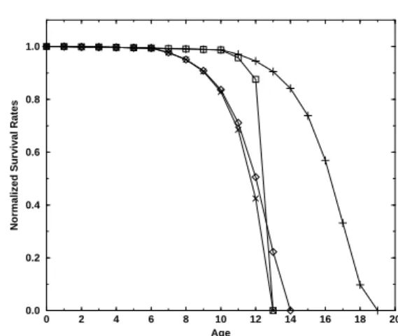
Figure 3 compares some different survival rates as a function of age. The common parameters are: R = 10,
T = 4,N(0) = 100,000(half for each sex in case of sexual
reproduction) andNmax = 10×N(0); birth rateb= 2in
asexual case andb = 4for females in sexual case (giving b = 2per individual as in the asexual one). In the sexual cases 6 randomly chosen positions were considered as the dominant ones.
0 1 0 1 0 0 1 0
0 0 1 1 1 1 0
1 2 3 4
0 0
0 1 1
0 1 1 1
1 0 0 0
1 1 0 1 0
1 0 1
1 0 0 0
0 0 1 1 1 0 1 1 1 0 0 0
1
1 2 3 4 2 3 4
(a)diploids (b)triploids (c)diploids with phenotype
Figure 2. Schematic representation of gamete formation for a) a diploid sexual population; b) for a triploid population; c) for a diploid sexual population with a non-age structured phenotype. Ar-rows indicate where mutations occurred. For diploids a second ga-mete is generated using this same strategy; for triploids the process is performed three times, generating one gamete per parent.
is shorter if menopause is considered, but there is no catas-trophic senescence: menopause sets in at age 12 and the total population survives until age 19. A crucial aspect of the model as well as in Nature is that sex is not transmitted genetically; independent of the genome we take each child as male with probability 1/2, and as female otherwise. So if death is hidden in the offspring genes, then either both males and females die soon, or both males and females die late. It is important to note that with this version of the model males and females present exactly the same survival rates, even if the male mutation rate is larger than the female one, and so neither Nature nor the model allows females to die sooner from accumulated genetic mutations than the males. How-ever, when both males and females reproduce from 10 to 32 (diamonds in Fig. 3), the whole population presents a larger life expectancy. In this case, we return to the same question, now slightly modified: Why does menopause exist?
0 0.2 0.4 0.6 0.8 1
0 5 10 15 20
Normalized Survival Rates
Age
Figure 3. Normalized survival rates for sexual and asexual repro-duction. Squares (m= 2) and x (m= 1) correspond to asexual
reproduction from age 10 to 12. Diamonds and + correspond to sexual reproduction,mf = mm = 1(one mutation from each
parent) and dominance = 6/32; diamonds for female reproduction from age 10 to 12 (males from 10 to 32) and stars for reproduction from age 10 to 32.
5
Self-organization of menopause
A possible explanation for menopause was already pointed out in 1957 by Williams [19]. He suggested that due to a reproduction risk that increases with advancing ages and a long period of child dependence, it is more advantageous to the females to cease reproduction in order to take care of the already born young offspring. This idea was simulated [20] by introducing into the Penna model the following restric-tions: a) there is a risk due to reproduction which is pro-portional to the number of current accumulated mutations (which means proportional to age, since in the model bad mutations accumulate at advancing ages); b) there is a pe-riod of parental care: offspring whose mothers die withing this period, are killed; c) the menopause age is no longer
imposed, but transmitted to the female offspring with muta-tions. That is, all the females start with a maximum repro-duction age (menopause age) equal to 32. When a daughter is born, it inherits the mother’s menopause age with proba-bility25%, or the mother’s menopause age±1 with prob-ability 75%. The minimum reproduction age is still im-posed and the same for both sexes, and the male maximum reproduction age is fixed at 32. With this strategy a self-organized distribution of menopause ages was obtained, as well as a period of post menopause survival. The distribu-tion of menopause ages is shown in Fig. 4. It is important to note in this figure that despite of the risk for later reproduc-tion, there is no self-organization of the menopause ages if there is no parental care. Both ingredients are necessary to obtain such an effect.
10 12 14 16 18 20 22 24 26 28 30 32
Menopause age 0.00
0.05 0.10 0.15 0.20
Percentage with menopause age
Figure 4. Percentage of females with a given menopause age as a function of the menopause age. Circles: parental care for 5 years; Diamonds: parental care for 4 years; Dotted line: no parental care.
6
Coevolution and the Red-Queen
hy-pothesis
the Penna model language, each individual carries two bit-strings that are read in parallel, as in the sexual case, and there are also recessive and dominant positions. During re-production, the bit-strings are cut in a random position, and two complementary pieces are jointed, forming the equiva-lent of a gamete in sexual reproduction (Fig. 2a). Then this same “gamete” is copied, generating the second bit-string of the baby, and random mutations are then introduced. It has been shown [21] that this kind of reproduction produces survival rates that are completely equivalent to those of the sexual case, besides being much faster and requiring much less effort.
A number of theories have been put forth to try to ex-plain the evolution and maintenance of sexual reproduction. In the center of this debate is the so-called “Red Queen” hypothesis, that relies heavily on the concept of diversity. In essence, it holds the action of genetically matching par-asites as responsible for creating a rapidly changing envi-ronment. In this unstable ecology only varieties that can mutate their genomic pool, at least as fast as the adaptation of the parasites proceed, can survive. The theory derives its name from this endless race, quoting from the Red Queen of Lewis Carol’s Alice in Wonderland: “It takes all the running you can do, to keep in the same place.” In fact, observations of competing varieties of a freshwater snail, Potamopyrgus antipodarum, have shown that there is a strong correlation between the prevalence of one reproduction regime and the concentration in its habitat of the trematode Microphallus, a parasite that renders the snail sterile by eating its gonads [22, 23, 24]. Namely, the asexual variety is predominant where the parasite appears in small concentrations, whereas higher concentrations of the trematode forces the species to prefer a sexual regime.
This correlation could be shown to exist in simulations of a conveniently modified Penna model [25]. The parasites are represented by a dynamically changing memory bank of genomes of some fixed number of entries. Each entry is modified if it comes into contact with the same genome twice in a row; in this case, it memorizes this pattern and stores it in the memory bank. At each time step, before the reproduction cycle, each female of the population is probed by a fixed numberEof randomly chosen entries of the par-asite bank. If one of these entries is a perfect match for the female’s genome, she is rended sterile and can no longer re-produce. The number of parasite exposuresEis an indirect measure of the parasite concentration in the habitat. For the host population, the reproductive regime of the females is no longer a fixed character, but can mutate with some small probability. That is, the offspring generated by a meiotic parthenogenetic female has a small probability to mutate to a sexual reproduction regime, and vice-versa. The simula-tions begin in the absence of the parasite infestation, and the initial population is set to have a sexual reproductive regime. As soon as the meiotic population appears, due to the muta-tions in the reproductive regime, it overrides the sexual va-riety: sex barely subsists due to infrequent back-mutations from the asexual variety. At some time step, the parasite in-festation is turned on. The resulting predominant variety is going to depend solely on the intensity of this infestation,
as measured by the exposure parameterE. For small val-ues ofE, the asexual variety has the upper hand. AsE is increased, a first-order transition is seen to a configuration dominated by the sexual population. Fig. 5 shows the frac-tion of females in the populafrac-tion that reproduces sexually, as a function of the exposure parameterE. The sudden jump in this fraction signals the order of the transition.
✁ ✄✂ ✆☎ ✆✝ ✟✞ ✄✠ ✂✁✡ ✂☞☛ ✂✟✌ ✂✁✍ ✂✁ ✂✟✂ ✡✏✎✡
✡✏✎✌ ✡✏✎ ✡✏✎☎ ✡✏✎✞ ☛✑✎✡
✒✓
✔✕
✖✗
✘
✙
✘✕
✗
✖
✚ ✛
✙ ✜
✢
✚
✙
✚
✖✗
✘
✙
✘✕
✗
✖
✚✛
✙ ✜
✣✥✤✧✦✩★✫✪✭✬✯✮✧✣✰✪
Figure 5. The fraction of females that reproduce sexually in the population is plotted against the value of the exposure parameter
E. The correlation between the dominant pattern of reproduction
and the intensity of the infestation, as measured by this last param-eter, is clearly seen.
It is easy to understand that the sexual reproduction gen-erates a larger genetic diversity than the meiotic partheno-genetic one, since the former involves two different indi-viduals instead of only one. In fact, it was already pointed by Stearns [26] that the meiotic parthenogenesis produces, in general, individuals that are homozygotous in all posi-tions. Because of this disadvantage, it is easier for the par-asites to contact twice the same genomic pattern among the asexual individuals than among the sexual ones. Of course such a conclusion gives rise to another question: Why are we diploids instead of triploids?
7
Diploids X Triploids
Since a diploid sexual population has the upper hand when competing against an asexual one due to the diversity gen-erated by the use of genetic material coming from two dif-ferent parents, why does not Nature enhance this effect by allowing the genome of the offspring to benefit from three different templates? Is the fact that for triploids mutations need to appear at the same position in the three homologous cromossomes (bit-strings) to be counted (except for dom-inant positions) enough to overcome the burden of using three individuals to generate one offspring? Simulations of a triploidal Penna population [27] have gathered arguments against this possibility.
parasites or any other external agent. This modification con-sists in assuming that harmful mutation reduces the survival probability. At each iteration, or “year,” each individual sur-vives with probabilityexp(−mǫ)if it has a total ofm harm-ful mutations (taking into account dominant positions) in it’s whole genome (it is killed if a random number is tossed that is smaller than the survival probability). ǫ is a parameter of the simulation, fixed from the start. To summarize, an individual may now die for any one of three reasons: i) ran-domly, due to the Verhulst logistic factor; ii) if its actual number of accumulated diseases reaches the limitT; iii) if its survival probability becomes too small.
In the triploid population, individuals have genomic ma-terial in three different bit-strings that are read in parallel. It is assumed that mating involves three individuals (two males and one female or vice-versa). Homozygous positions are those with three equal bits at homologous loci. Harmful mu-tations are active only if there are three bits1 at that same position, or at a heterozygous locus at which harmful muta-tions are dominant. Only females generate offspring. Cross-ing and recombination are performed by a random choice of a locus at which the three strings are cut, generating six pieces. Two complementary pieces of those are randomly chosen to form one gamete. This process is performed for each one of the three parents. Deleterious mutations are ran-domly introduced in each gamete (see Fig. 2b). The baby is a male or a female, with equal probability.
Figure 6 presents the time evolution of a diploid sexual population and of two different triploid ones, showing that the diploid sexual population is larger than any of the other two.
399000 399200 399400 399600 399800 400000
Time 4500
5500 6500 7500 8500 9500
Individuals
Figure 6. Time evolution of a diploid population (upper curve) and two triploid populations: in the central curve, reproduction in-volves one male and two females, while in the lower one it inin-volves one female and two males.
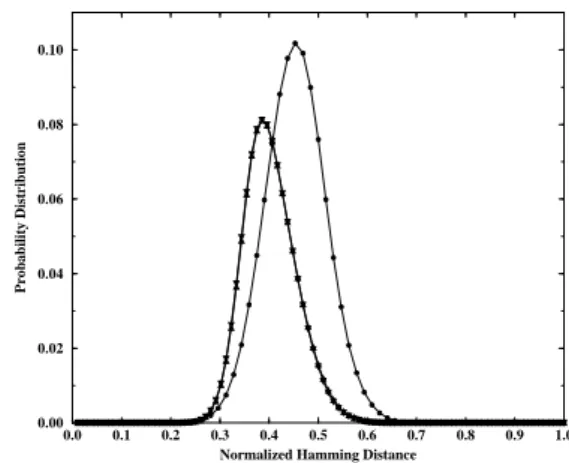
The genetic diversity is obtained computing the Ham-ming distance, in this case defined by the number of dif-ferent loci (bits) between the genomes, for all pairs of in-dividuals. The probability distribution of these distances is obtained by making a histogram of the fraction of pairs, out of all possible pairs in the population, that present a given Hamming distance, normalized by its maximum possible
value (64 for diploids and 96 for triploids). Fig. 7 shows the resulting distributions for the diploid and triploid popu-lations. It is clear that the diploid population presents both a larger mean distance between pairs, indicated roughly by the position of the peak of the distribution, and a larger vari-ance, measured by the width at half the maximum height of the curves. The results are essentially the same if a double crossing of the triploid genome is performed during repro-duction, and there is no benefit for the triploids to ensure that the offspring have their genetic material gathered from all three parents.
0.0 0.1 0.2 0.3 0.4 0.5 0.6 0.7 0.8 0.9 1.0 Normalized Hamming Distance
0.00 0.02 0.04 0.06 0.08 0.10
Probability Distribution
Figure 7. Genetic diversity of a diplod population (full circles) and of the two triploid populations mentioned in the captions of the previous figure, which are, for this particular measure, indistin-guishable.
The diploid population also presented a slightly better survival rate, with comparable longevities [27]. These re-sults show that genetical reproduction has to recombine ma-terial in the correct amount, in order to balance the extra cost of reproduction involved when multiple parents are needed - more is not necessarily better!
8
Sympatric speciation with
pheno-typic selection
Penna model to represent phenotypic selection and specia-tion.
The version with a single phenotypic trait [29] was mo-tivated by field observations. The intention was to mimic the seasonal effect of rainfall on the availability of seeds of different sizes in the Galapagos islands and its impact on the morphology of beak sizes in the population of ground finches that feed on these seeds [30, 31, 32]. It has been ob-served that depending on the amount of rain, the distribution of seed sizes changes from a broad distribution centered at middle sized seeds to a double-peaked distribution, of only small or large seeds. The beak sizes of the ground finches follow this same dynamics in a very impressive and fast (few generations) process of adaptation.
The beak is represented by a single pair of non age-structured bit-strings, added to the chronological genome of each individual. The dynamics of reproduction and muta-tions are the same for both the age-structured and the new strings - for the latter, a mutation that changes a bit from
1 to0is also allowed (see fig.4c). The beak size is deter-mined by counting, in this non-structured pair of bit-strings, the number of recessive bit-positions (chosen as16) where both bits are set to1, plus the number of dominant positions with at least one of the two bits set. It will be a numberk between0, meaning a very small beak, and32, for a very large one. Its selective value is given by a fitness function F(k), that indicates how much the individual is fitted to the environment. For a given value of the beak size k, F(k)
quantifies the availability of seeds for individuals with that particular morphology.
This quantification was done through the Verhulst fac-tor, which now becomes dependent on genetic material (the beak size). It gives the probability of death by intra-specific competition at each time step:
V(t) = N(t, k)
(Nmax∗F(k))
,
whereN(t, k)is the number of individuals of beak sizekat time stept.
The simulations were done with two different functional forms for the functionF(k). At the beginning of the sim-ulations,F(k)is a single-peaked function with a maximum atk = 16, representing large availability of medium-sized seeds:
F(k) = 1−16−k
A , k <16
= 1−k−16
A , k≥16 (1)
whereAis a constant that controls the intensity of the envi-ronment pressure.
After20 000time steps, there is a sudden change in the pattern of seed availability (simulating the variation in the rainfall regime). The fitness function that expresses this new pattern is, for instance,
F′(k) = 1−A−16 +k
A , k <16
= 1−A−k+ 16
A , k≥16 (2)
This change force evolution to give rise to a polymor-phism, shown in Fig. 8 (diamonds) as a resulting2-peaked equilibrium distribution of beak sizes. This polymorphism is reversible: if, in a subsequent time step, the pattern of avail-ability of edible seeds reverts to its original configuration, so does also the distribution of beak sizes.
0 10 20 30
Beak size 0
0.1 0.2 0.3 0.4 0.5
Frequency
Middle sized seeds abundant F(k)
Small or big seeds abundant F’(k)
Figure 8. The distribution of phenotypes in the population is shown for two different regimes of seed availability. The circles corre-spond to the equilibrium population at time step12 000, in a situ-ation in which seeds are available for a broad distribution of sizes, peaked at beak sizek = 16; the corresponding fitness function F(k), adequately rescaled to fit in the graph, is shown for a
com-parison. The two-peaked phenotype distribution corresponding to the diamonds, is a snap-shot of the population at time step50 000, that is, after F(k) has been double-peaked for30 000time steps. The population has already split into a (reversible) polymorphism, with two different beak sizes. Since there is no reproductive iso-lation, mating between birds feeding on different niches generate offspring with medium-sized beaks, represented by the small bump atk= 16).
In order to really have speciation, which implies in a non reversible polymorphism, it was necessary to introduce sex-ual selection into the reproductive strategy, to avoid mating between small and large beaks. A single locus was intro-duced into the genome that codes for this selectiveness, also obeying the general rules of the Penna model for genetic heritage and mutation. If it is set to0, the individual will not be selective in mating (random mating), and it will be se-lective (assortative mating) if this locus is set to1. The mu-tation probability for this locus was set to0.001in all sim-ulations. Individuals that are selective will choose mating partners with its same morphological characteristics, that is, if an individual hask <(>)16and is selective, it will only mate with a partner that also hask <(>)16.
population, it was observed that the fraction of selective in-dividuals increased to at most0.003whileF(k)was single-peaked, and jumped to nearly 1.0 after the establishment
of a double-peaked distribution of seeds. Two distinct pop-ulations, each of which does not mate with a partner from the other, is the final result: evolutionary dynamics made it advantageous to develop assortative mating in this bi-modal ecology, and as a consequence of reproductive isolation, one single species has split into two.
Both a simpler and a more elaborated model (with two phenotypic traits) using the Penna bit-string strategy to sim-ulate sympatric speciation can be found in [33].
9
Conclusions
We have presented the Penna model for biological age-ing and some of its most important results. Ageage-ing is an unavoidable process (experimentally confirmed by the au-thor) and has been extensively studied by many different scientists, since a very long time. Although the evolution-ary theories for senescence have appeared around 1950, Monte Carlo Simulations on this subject started only after the publication of the Partridge-Barton analytical mathemat-ical model [34] in 1993. The Penna model is now the most widespread Monte Carlo technique to simulate and study the different aspects of population dynamics, including ageing. In this review we have focused attention on results concern-ing the differences between reproductive regimes and the advantages of sexual reproduction, as well as on the mod-ifications introduced into the Penna model in order to study sympatric speciation.
Acknowledgments: to P.M.C. de Oliveira, D. Stauf-fer, T.J.P. Penna, J.S. S´a Martins, A.T. Bernardes and A.O. Sousa for many discussions and collaborations along the last years; to the Brazilian agencies CNPq, FAPERJ and CAPES for financial support.
References
[1] Luca Peliti, cond-mat/97122027 (1997). [2] M. Eigen, Naturwissenchaften 58, 465 (1971).
[3] S. Moss de Oliveira, Domingos Alves, and J.S. S´a Martins, Physica A285, 77 (2000).
[4] P. Bak and K. Sneppen, Phys. Rev. Lett. 71, 4083 (1993). [5] P. Bak, How Nature works: The science of self-organized
criticality, Oxford University Press, Oxford/Melbourne/
Tokyo (1997).
[6] T.J.P. Penna, J. Stat. Phys. 78, 1629 (1995).
[7] K.W. Watcher and C.E. Finch, Between Zeus and the Salmon.
The Biodemography of Longevity, National Academy Press,
Washington DC (1997).
[8] N.J. Holbrook, G.R. Martin, and R.A. Lockshin, Cellular
Ageing and Death, Wiley-Liss, New York (1996).
[9] M.Ya. Azbel, Proc. Natl. Acad. Sci. USA 91 12453 (1994). [10] M.R. Rose, Evolutionary Biology of Aging, Oxford
Univer-sity Press, New York (1991).
[11] T.J.P. Penna and S. Moss de Oliveira, J. Physique I 5, 1697 (1995).
[12] T.J.P. Penna, S. Moss de Oliveira, and D. Stauffer, Phys. Rev. E 52, R3309 (1995).
[13] M. Lynch and W. Gabriel, Evolution 44, 1725 (1990). [14] P. Pamilo, M. Nei, and W.H. Li, Genet. Res., Camb. 49, 135
(1987).
[15] S. Moss de Oliveira, P.M.C. de Oliveira, and D. Stauffer,
Evo-lution, Money, War and Computers, Teubner, Leipzig (1999).
[16] A.T. Bernardes, J. Physique I 5, 1501 (1995). [17] A.T. Bernardes, Ann. Physik 5, 539 (1996).
[18] D. Stauffer, P.M.C. de Oliveira, S. Moss de Oliveira, and R. M. Zorzenon dos Santos, Physica A231, 504 (1996). [19] G.C. Williams, Evolution 11, 398 (1957).
[20] S. Moss de Oliveira, A.T. Bernardes, and J.S. S´a Martins, Eur.Phys.J. B7, 501 (1999).
[21] A.T. Bernardes, J. Stat. Phys. 86, 431 (1997).
[22] C.M. Lively, E.J. Lyons, A.D. Peters, and J. Jokela, Evolu-tion 52, 1482 (1998).
[23] M.F. Dybdahl and C.M. Lively, Evolution 52 1057 (1998). [24] R.S. Howard and C.M. Lively, Nature (London) 367, 554
(1994).
[25] J.S. S´a Martins, Phys. Rev. E61, R2212 (2000).
[26] S.C. Stearns, The Evolution of Sex and its Consequences, Birkhauser, Basel (1987).
[27] A.O. Sousa, S. Moss de Oliveira, and J.S. S´a Martins, Phys. Rev. E67, Art. No. 032903, (Mar. 2003).
[28] J.S. S´a Martins and D. Stauffer, Physica A294, 191 (2001). [29] J.S. S´a Martins, S. Moss de Oliveira, and G.A. de Medeiros,
Phys.Rev. E64 (2001) 021906
[30] P.T. Boag and P.R. Grant, Nature 274, 793 (1978); P.T. Boag and P.R. Grant, Science 214, 82 (1981).
[31] P.R. Grant, Ecology and evolution of Darwin’s finches, Princeton University Press, Princeton, USA (1986). [32] D. Lack, Darwin’s Finches, Cambridge University Press,
Cambridge, England (1983).