J. Braz. Soc. Mech. Sci. & Eng. vol.34 número3

(1)

V. N. Gaitonde

gaitondevn@yahoo.co.in Department of Industrial & Production Engineering B.V.B. College of Engineering and Technology Hubli-580 031, Karnataka, India

S. R. Karnik

karniksr@yahoo.com Department of Electrical & Electronics Engineering B.V.B. College of Engineering and Technology Hubli-580 031, Karnataka, India

Selection of Optimal Process

Parameters for Minimizing Burr Size in

Drilling Using Taguchi’s Quality Loss

Function Approach

The exit burr in drilling degrades the precision of products and causes additional cost of deburring. Therefore, it is essential to minimize burr size at the exit of holes in drilling at the manufacturing stage. Taguchi’s quality loss function approach, a multi-response optimization method, has been employed to determine the best combination values of cutting speed, feed, point angle and lip clearance angle for specified drill diameters to simultaneously minimize burr height and burr thickness during drilling of AISI 316L stainless steel workpieces. The experiments were planned as per L9 orthogonal array and multi-response signal to noise (S/N) ratio was applied to measure the performance characteristics. Analysis of means (ANOM) and analysis of variance (ANOVA) were performed to determine the optimal levels and to identify the level of importance of parameters. The confirmation tests with the optimal levels of parameters were carried out to illustrate the effectiveness of Taguchi optimization.

Keywords: AISI 316L stainless steel, drilling, burr size, Taguchi’s quality loss function, ANOVA

Introduction1

Drilling is one of the most common and complex operations among many kinds of machining methods. Burr is a plastically deformed material generated on part edge during drilling (Gillespie, 1975). The exit burr is formed on the other side of drilled hole, when the drill pierces the workpiece by pushing out uncut volume. The exit burrs in drilling affect the reliability of product and degrade the performance in the precision parts. The special tools are necessary for deburring to remove the burrs formed inside a cavity. It is estimated that the deburring and edge finishing costs on precision components constitute as much as 30% of total cost of finished products (Gillespie, 1979). Thus, it is essential to minimize the burr formation at the manufacturing stage by selecting the appropriate drilling process parameters. This necessitates an appropriate optimization tool to minimize the burr size for a specified combination of drilling process parameters.

Many researchers have carried out experimental investigations to study the effects of process factors on burr formation mechanisms during drilling of several workpiece materials (Stein and Dornfeld, 1997; Dornfeld et al., 1999; Lin, 2002; Ko et al., 2003). In order to analyze the burr formation mechanisms in drilling, finite element models were employed (Guo and Dornfeld, 2000; Min et al., 2001a). The empirical drilling charts were developed to minimize burr size for a single layered material to choose suitable cutting conditions for different materials (Min et al., 2001b; Min et al., 2001c; Kim et al., 2001). The mathematical models based on response surface methodology (RSM) were also developed for predicting and analyzing the burr size in drilling (Pande and Relekar, 1986). The investigations on drilling optimization of stainless steel workpieces using genetic algorithms (GA) revealed that point angle and lip clearance angle have major contributions in controlling the burr size apart from the cutting conditions (Gaitonde et al., 2008). However, GA optimization requires an accurate model to describe the complex and non-linear relationship between the process parameters and burr size.

Taguchi parameter design has produced a unique and powerful optimization tool that differs from conventional practices and can economically satisfy the needs of problem solving and design optimization with less number of experiments (Phadke, 1989; Ross, 1996). Thus, it is possible to reduce time and cost of experimental investigations and also to improve the performance characteristics

Paper received 10 August 2009. Paper accepted 9 November 2009 Technical Editor: Anselmo Diniz

using Taguchi design. The original Taguchi technique is designed to optimize a single performance characteristic. However, most of the processes have several performance characteristics and hence there is a need to obtain single optimal process parameter combination setting. Several modifications were suggested to original Taguchi method for multi response optimization (Jeyapaul et al., 2005). The methodology of Taguchi’s quality loss function has proved to be an attractive and efficient optimization tool for multiple performance characteristics (Ames et al., 1997). The multi-performance characteristic optimization using Taguchi’s quality loss function employs the weighting factors in the total loss function to obtain multi-response signal to noise (S/N) ratio.

AISI 316L stainless steel material has high corrosive resistance properties and hence finds many applications in chemical industries, aircraft designs and in manufacture of medical apparatus. The formation of burrs during drilling is a major problem due to large strain hardening coefficients and ductility of the work materials. One of the most common cutting tool materials for drilling of stainless steel is HSS (Kim et al., 2001). Hence, HSS conventional twist drills were used for drilling experiments.

This paper presents the application of Taguchi’s quality loss function concept for multi-objective drilling process optimization to determine the best combination values of cutting speed (v), feed (f), point angle (θ) and lip clearance angle (ψ) for a given drill diameter in order to simultaneously minimize burr height (Bh) and burr

thickness (Bt) during drilling of AISI 316L stainless steel

workpieces using high speed steel (HSS) twist drills.

Nomenclature

Bh = burr height, mm Bt =burr thickness, mm CI = confidence interval d = drill diameter, mm f = feed, mm/rev k = number of factors

Lij = quality loss function for the ith quality characteristics at the jth_trial

l = number of levels for each factor

Nij =inormalized quality loss associated with ith quality characteristic at jth trial

(2)

Ve = mean square of pooled error Greek Symbols

j

η

= multi-response S/N ratio for jth trial

θ = point angle, degree ψ = lip clearance angle, degree

υ

= degrees of freedom

Methodology

Taguchi parameter design

Taguchi parameter design is an effective methodology for finding the optimum levels of controllable factors to make the product or process insensitive to noise factors (Phadke, 1989; Ross, 1996). Taguchi method is based upon orthogonal array experiments, which allows the simultaneous effect of several process parameters. Taguchi suggests S/N ratio as the objective function for orthogonal array experiments and to measure the quality characteristics. The S/N ratio also indicates the degree of predictable performance in the presence of noise factors. Taguchi classifies the signal to noise ratio into smaller the better type, larger the better type and nominal the best type based on the type of objective function (Phadke, 1989; Ross, 1996).

The analysis of means (ANOM) is used to determine the optimal levels of the process parameters in Taguchi design. The ANOM is also used for estimating the main effects of each parameter, and the effect of a factor level is the deviation it causes from the overall mean response (Phadke, 1989). The process parameter setting with the highest value of S/N ratio is the optimal quality with minimum variance in the experimental design space. The analysis of variance (ANOVA) in Taguchi analysis establishes the relative importance of process parameters and is performed on S/N ratios to obtain the percentage contribution (PC) of each of the parameters (Phadke, 1989; Ross, 1996).

Multi-response optimization using quality loss function

The multi-performance characteristic optimization using Taguchi’s quality loss function employs the weighting factors in total loss function (Ames et al., 1997). Taguchi used a loss function to determine the deviation between the experimental and desired values. This loss function is further transformed into a multi-response S/N ratio. In the process optimization with multiple performance characteristics, each performance characteristic may belong to a different category in the analysis of S/N ratio.

In the present work, the objective is to simultaneously minimize burr height and burr thickness at the exit of holes in drilling. The simultaneous minimization of performance characteristics is obtained by considering lower the better type category (Phadke, 1989; Ross, 1996). The quality loss function for the ith quality characteristics at the jth trial in an orthogonal array for lower the better type is given as:

2 ij ij z

L = (1)

where zij is the ith performance characteristic value in the jth trial.

In a process with multiple responses, the loss function for every performance characteristic is normalized and the normalized quality loss associated with ith quality characteristic at jth trial is given by:

_ i ij ij

L L

N = (2)

where = ∑

=

n 1 i ij i

_

L n 1

L is the average loss function of ith characteristic

due to n trials.

In the weighting method of computing total quality loss function, proper weighting factors to each of the normalized quality loss function are to be assigned. For g number of performance characteristics, the total loss function for jth_{trial is given as:}

∑

= =

g 1 i i ij

j wN

TL (3)

where wi is the scalar weighting factor for ith performance

characteristic. Taguchi loss function for multi-response optimization requires the maximization of response S/N ratio. The multi-response S/N ratio for jth trial can be expressed as:

) TL ( log

10 10 j

j =

-η (4)

Experimental Procedure

Experimental parameters and their levels

In the present study, four process parameters, namely, cutting speed (v), feed (f), point angle (θ) and lip clearance angle (ψ) were identified. The drilling of AISI 316L stainless steel work material is usually performed in the industries with cutting speed in the range 8-24 m/min using HSS twist drills. The feed in the range 0.04-0.12 mm/rev is normally preferred with higher drill diameters in order to avoid excessive temperature rise during drilling operation. The range of point angle for drilling of stainless steel was selected based on the investigations carried out by Stein (1997). The range of lip clearance angle was fixed as 8-12°based on preliminary experiments. Accordingly, the ranges of the process parameters were selected in the present investigation. Each parameter was investigated at three levels to study the non-linearity effect of process parameters. The identified process parameters and their levels are given in Table 1.

Table 1. Process parameters and their levels.

Code Parameters Levels

1 2 3

A Cutting speed (v), m/min 8 16 24

B Feed (f), mm/rev 0.04 0.08 0.12

C Point angle (θ), 0 118 126 134

D Lip clearance angle (ψ), 0 8 10 12

Planning for experiments

Taguchi parameter design begins with the selection of orthogonal array with number of levels (l) defined for each of process parameters v, f, θ and ψ. The minimum number of trials in an orthogonal array is given by:

1 k ) 1 l (

N_min= − + (5)

where, k = number of parameters = 4. This gives Nmin = 9 and hence,

according to Taguchi quality design concept (Phadke, 1989; Ross, 1996). L9 orthogonal array has been selected, which has 9 rows

corresponding to number of test trials with required columns. The experimental layout for drilling process parameters using L9

(3)

Table 2. Experimental layout of process parameters as per L9 orthogonal array.

Trial no. Levels of process parameters

A B C D

1 1 1 1 1

2 1 2 2 2

3 1 3 3 3

4 2 1 2 3

5 2 2 3 1

6 2 3 1 2

7 3 1 3 2

8 3 2 1 3

9 3 3 2 1

Experimentation and Burr Size Measurement

The drilling experiments were performed on a three-axis

‘YCM-V116B’ CNC vertical machining center (Make: Yeong Chin

Machinery Industries Co., Taiwan) with a Fanuc controller. The CNC machine is equipped with a 15 kW drive motor. The machining center has a maximum feed rate of 5000 mm/min and a spindle speed from 45-4000 rpm. The maximum table travel along X-axis is 1100 mm and along Z-axis is 630 mm. The maximum saddle travel along Y-axis is 600 mm. A drilling fixture was used to clamp the specimens onto a flat surface and the purpose is to maintain the perpendicularity of the exit surface of the hole and spindle of the machine. The fixture consists of two clamps, which can be tightened to hold the edge of the specimen onto the flat surface. The fixture contained a slot in between the flat surfaces on which the specimen rested. The seat of the fixture was perfectly ground to create a flat surface perpendicular to the spindle before mounting the specimen for drilling. The fixture was mounted in the vise on the machine tool table.

The 25 mm thick AISI 316L stainless workpieces were used for all drilling experiments. The chemical composition and mechanical properties of the work material are listed in Table 3. The work specimens were annealed at 1060 ± 10°C, soaked for one hour and then quenched in water. The workpieces were polished on the exit surfaces before drilling to prepare for the optical burr measurement.

Table 3. Chemical composition and mechanical properties of AISI 316L stainless steel.

Chemical composition (wt%)

0.026 C, 0.37 Si, 1.6 Mn, 0.029 P, 0.027 S, 16.55 Cr, 10.0 Ni, 2.02 Mo, 0.16 Co, 0.036 N

Mechanical properties

Tensile strength: 582 - 591 MPa Yield strength: 300 - 331 MPa Elongation: 53%

Hardness: 170 BHN Reduction of area: 73%

HSS parallel shank stub series twist drills (Make: Addison & Co. Ltd., India) confirming to IS: 5100/DIN: 1897/BS: 328/ I. S. O specifications were used for the experimentation. The different point angle and lip clearance angles were ground as per orthogonal array. ‘Cut60EP’ water-soluble oil was used as coolant throughout the experimentation.

The burr height and burr thickness were measured on ‘RPP-400’ toolmakers’ microscope (Make: Sicherun-Gen Versehen, Germany) with a resolution of 1 µm at 30

×

magnification. To measure burr height, the focus was put on top of burr and then on exit surface. The burr height is the distance between two foci. The burr thickness was measured by reading the distance between inner surface of drilled hole and the location at which curvature of root of burr begins. The observed burrs were more or less uniform during the drilling experiments. The burr height (Bh) and burr thickness (Bt)

values were recorded at four equally spaced locations around the circumference and the mean reading was the process response. In order to avoid systematic errors, the trials were randomized. The measured values of burr height and burr thickness corresponding to

L9 orthogonal array for selected drill diameters of 4, 10, 16, 22 and

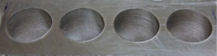
28 mm are illustrated in Table 4. The burrs observed at the exit of holes during experimentation for 16 mm drill diameter are illustrated in Fig. 1.

Figure 1. The observed burrs at the exit of holes during drilling experimentation for 16 mm drill diameter.

Results and Discussion

Analysis of experimental data

In order to optimize the multiple performance characteristics, namely, Bh and Bt, Taguchi’s quality loss function concept has been

employed in the present study. The loss functions, normalized loss functions for each of the responses, total loss function and corresponding multi-response S/N ratios for each trial of L9

orthogonal array were determined using Eqs. (1)-(4) and are presented in Tables 5, 6, 7, 8, and 9 for drill diameters of 4, 10, 16, 22 and 28 mm respectively. In the present investigation, total loss function was computed using weighting factor of 0.5, which gives an equal importance to both Bh and Bt.

Analysis of means and analysis of variance

(4)

Table 4. Measured values of burr height and burr thickness for different drill diameters.

Trial no. (j)

d = 4 mm d = 10 mm d = 16 mm d = 22 mm d = 28 mm

Bh

(mm)

Bt

(mm)

Bh

(mm)

Bt

(mm)

Bh

(mm)

Bt

(mm)

Bh

(mm)

Bt

(mm)

Bh

(mm)

Bt

(mm)

1 0.103 0.021 0.127 0.135 0.056 0.126 0.236 0.072 0.561 0.059

2 0.321 0.156 0.228 0.102 0.172 0.152 0.223 0.176 0.242 0.121

3 0.929 0.155 0.752 0.186 0.547 0.269 0.444 0.309 0.210 0.307

4 0.583 0.217 0.521 0.166 0.461 0.246 0.507 0.281 0.657 0.294

5 0.816 0.197 0.545 0.085 0.353 0.134 0.265 0.081 0.319 0.049

6 0.455 0.206 0.312 0.170 0.368 0.199 0.572 0.184 0.791 0.120

7 0.791 0.208 0.584 0.165 0.379 0.214 0.305 0.219 0.362 0.162

8 0.607 0.173 0.417 0.139 0.513 0.194 0.713 0.209 0.983 0.181

9 0.517 0.251 0.326 0.152 0.288 0.150 0.355 0.105 0.526 0.036

Table 5. Computed values of multi-response S/N ratio for d = 4 mm.

Trial no. (j)

Loss function

Normalized loss function

Total loss function (TLj)

Multi-response S/N ratio (ηj), dB

L1j L2j N1j N2j

1 0.010609 0.000441 0.027669 0.012667 0.020168 16.9534

2 0.103041 0.024336 0.268734 0.69902 0.483877 3.152649

3 0.863041 0.024025 2.250837 0.690087 1.470462 -1.67454

4 0.339889 0.047089 0.886441 1.352571 1.119506 -0.49026

5 0.665856 0.038809 1.736573 1.114738 1.425656 -1.54015

6 0.207025 0.042436 0.539927 1.218919 0.879423 0.55802

7 0.625681 0.043264 1.631795 1.242703 1.437249 -1.57532

8 0.368449 0.029929 0.960926 0.859672 0.910299 0.408159

9 0.267289 0.063001 0.697098 1.809622 1.25336 -0.98076

Trial no. (j)

Loss function

L1j L2j N1j N2j

1 0.016129 0.018225 0.075579 0.834495 0.455037 3.419532

2 0.051984 0.010404 0.243593 0.476383 0.359988 4.437119

3 0.565504 0.034596 2.649906 1.584098 2.117002 -3.25721

4 0.271441 0.027556 1.27195 1.261747 1.266849 -1.02725

5 0.297025 0.007225 1.391835 0.330822 0.861328 0.648313

6 0.097344 0.0289 0.456146 1.323287 0.889717 0.507483

7 0.341056 0.027225 1.598161 1.246591 1.422376 -1.53014

8 0.173889 0.019321 0.81483 0.884679 0.849754 0.707066

9 0.106276 0.023104 0.498001 1.057897 0.777949 1.09049

Trial no. (j)

Loss function

L1j L2j N1j N2j

1 0.003136 0.015876 0.021818 0.427296 0.224557 6.486736

2 0.029584 0.023104 0.205821 0.621835 0.413828 3.831803

3 0.299209 0.072361 2.081649 1.947567 2.014608 -3.0419

4 0.212521 0.060516 1.478545 1.628763 1.553654 -1.91354

5 0.124001 0.017001 0.862696 0.457578 0.660137 1.803659

6 0.135424 0.039601 0.942168 1.065845 1.004006 -0.01736

7 0.143641 0.045796 0.999335 1.232581 1.115958 -0.47648

8 0.263169 0.037636 1.830912 1.012958 1.421935 -1.5288

(5)

Trial no. (j)

Loss function

L1j L2j N1j N2j

1 0.055696 0.005184 0.297585 0.137899 0.217742 6.620577

2 0.049729 0.031625 0.265703 0.788268 0.527067 2.782265

3 0.197136 0.095481 1.053303 2.539876 1.79659 -2.54449

4 0.257049 0.078961 1.37342 2.10043 1.736925 -2.39781

5 0.070225 0.006561 0.375214 0.174528 0.274871 5.608708

6 0.327184 0.033856 1.748153 0.900599 1.324376 -1.22011

7 0.093025 0.047961 0.497035 1.275804 0.886419 0.523608

8 0.508369 0.043681 2.71623 1.161952 1.939091 -2.87598

9 0.126025 0.011025 0.673355 0.293274 0.483315 3.157699

Trial no. (j)

Loss function Normalized loss

function

L1j L2j N1j N2j

1 0.314721 0.003481 0.960008 0.113548 0.536778 2.702052

2 0.058564 0.014641 0.17864 0.477581 0.328111 4.839793

3 0.0441 0.094249 0.13452 3.074351 1.604435 -2.05322

4 0.431649 0.086436 1.316679 2.819495 2.068087 -3.15569

5 0.101761 0.002401 0.310406 0.078319 0.194363 7.113869

6 0.625681 0.0144 1.908544 0.46972 1.189132 -0.7523

7 0.131044 0.026244 0.39973 0.856065 0.627897 2.021115

8 0.966289 0.032761 2.947516 1.068646 2.008081 -3.02781

9 0.276676 0.001296 0.843958 0.042275 0.443116 3.534824

Figure 2. Response graph of multi-response S/N ratio for burr size (d = 4 mm). Figure 3. Response graph of multi-response S/N ratio for burr size (d = 10 mm).

1 2 3

-2 -1 0 1 2 3 4 5 6 7

Level

S

/N

r

a

ti

o

Drill diameter = 4 mm

Cutting speed Feed

Point angle

Lip clearance angle Overall mean

1 2 3

-1.5 -1 -0.5 0 0.5 1 1.5 2

Level

S

/N

r

a

ti

o

(6)

Figure 4. Response graph of multi-response S/N ratio for burr size (d = 16 mm).

Since ANOVA has resulted in zero degree of freedom for error term, it is necessary to pool the parameter having less influence for correct interpretation of results. It can be seen from the ANOVA tables that point angle and lip clearance angle have significant effects in minimizing the burr size. On the other hand, cutting speed and feed have moderate effects in controlling the burr size.

Verification experiments

To predict and verify the performance characteristic using optimal level of design parameters, the predicted optimum value of S/N ratio (ηopt) is determined and is given by (Phadke, 1989; Ross, 1996):

∑ −

+ =

=

p

1

j i,j max opt m [(m ) m]

η

(6)

where (mi,j)max is the S/N ratio of optimum level i of factor j and p is

number of main design parameter that affects the burr size.

Table 10. Results of ANOVA for burr size (d = 4 mm).

Factor DOF SS MS Pure

sum PC

A 2 91.13 45.57 43.52 15.42

B 2 52.34 26.17 4.73 1.68

C 2 91.25 45.63 43.65 15.46

D 2 47.60 23.80 - -

Error 0 0 - - -

Pooled error (2) (47.60) (23.80) - -

Total 8 282.32 35.29 - -

Table 11. Results of ANOVA for burr size (d =10 mm).

sum PC

A 2 4.30 2.15 - -

B 2 9.58 4.79 5.269 11.71

C 2 16.85 8.43 12.54 27.88

D 2 14.25 7.13 9.94 22.10

Error 0 0 - - -

Pooled error (2) (4.30) (2.15) - -

Total 8 44.98 5.62 - -

sum PC

A 2 11.75 5.88 6.56 8.81

B 2 5.20 2.60 - -

C 2 9.16 4.58 3.97 5.32

D 2 48.36 24.18 43.17 57.98

Error 0 0 - - -

Pooled error (2) (5.20) (2.60) - -

Total 8 74.47 9.31 - -

sum PC

A 2 6.74 3.37 6.45 6.22

B 2 7.26 3.63 6.98 6.73

C 2 0.28 0.14 - -

D 2 89.42 44.71 89.14 85.96

Error 0 0 - - -

Pooled error (2) (0.28) (0.14) - -

Total 8 103.70 12.96 - -

1 2 3

-3 -2 -1 0 1 2 3 4

Level

S

/N

r

a

ti

o

Drill diameter = 16 mm Cutting speed Feed Point angle Lip clearance angle Overall mean

1 2 3

-3 -2 -1 0 1 2 3 4 5 6

Level

S

/N

r

a

ti

o

Drill diameter = 22 mm Cutting speed Feed Point angle Lip clearance angle Overall mean

1 2 3

-3 -2 -1 0 1 2 3 4 5

Level

S

/N

r

a

ti

o

(7)

sum PC

A 2 1.60 0.80 - -

B 2 13.56 6.78 11.96 11.09

C 2 12.19 6.10 10.59 9.82

D 2 80.47 40.24 78.87 73.15

Error 0 0 - - -

Pooled

error (2) (1.60) (0.80) - -

Total 8 107.83 13.48 - -

The confidence interval (CI) is determined to judge the closeness of observed S/N ratio (ηobs) value with that of predicted

value (ηopt) and is given by (Ross, 1996):

) n

1 n

1 ( V F CI

ver eff e ) e , 1

( +

= υ (7)

where ₎

e , 1 (

F

_υ

is the Fisher value for 95% confidence interval,

e

υ

is the degrees of freedom for pooled error, V_e is the mean square of pooled error,

υ + =

1 N eff

n , N is the total trial number in

orthogonal array, υ is the degrees of freedom of p factors and

ver

n is the confirmatory test trial number.

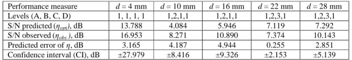
Here, the best combination values of the process parameters obtained through Taguchi optimization were set for the selected drill diameters and the workpieces of the same batches were drilled. The observed value of S/N ratio (ηobs) is compared with that of the

predicted value (ηopt). Table 15 illustrates the confirmatory test

results for the selected drill diameters. It is observed from the table that the prediction error, i.e., the difference between ηopt and ηobs, is

within CI value, indicating the adequacy of the burr size models.

Discussion on optimization results

From Taguchi optimization results, it is found that the optimal values of cutting speed and lip clearance angle are at low levels i.e. cutting speed at 8 m/min and lip clearance angle at 80 for all the drill diameters specified. On the other hand, the requirement of feed is low (0.04 mm/rev) for a 4 mm drill diameter and medium level (0.08 mm/rev) for other drill diameters. Further, it is also observed that larger point angle is required for higher drill diameters beyond 16 mm in order to minimize the burr size.

It is obvious that at higher cutting speed temperature increases with the increase in feed, which helps the material to deform more easily and thus increase in burr size. The low values of lip clearance

angle provide enough support for drilling edges, causing the drill to easily break the chips, resulting into smaller burrs. Further, low values of feed ensure minimum thrust, which in turn determines the amount of material that undergoes the plastic deformation. The larger point angles assure maximum lip movement in the earliest possible time to avoid work hardening, resulting into small burrs due to change in chip flow direction. Further, the larger point angles at higher drill diameter values induce the axial chip flow direction, which results the strain at the drill point that is smaller than the exit edge of the hole, giving rise to smaller burrs.

From the above discussions it is evident that the requirement of process parameters to minimize burr size is different for different drill diameters. Thus, with proper selection of process parameters, it is possible to minimize the burr size at all drill diameter values specified.

Conclusions

Taguchi’s quality loss function approach, a multi-response optimization method, has been employed in the present investigation to determine the best combination values of process parameters for simultaneously minimizing the burr height and burr thickness at the exit of holes in drilling of AISI 316L stainless steel with HSS twist drills. The experiments were planned as per L9 orthogonal array

under different conditions of cutting speed, feed, point angle and lip clearance angle for specified drill diameter. The optimal levels of process parameters were identified through ANOM and the relative significance of the process parameters was determined by ANOVA. The following conclusions are drawn from the present investigation within the ranges of the process parameters selected:

• The optimal values of cutting speed and lip clearance angle are at low level, i.e. 8 m/min and 8° respectively, for all the drill diameters specified. Further, from ANOM it is also observed that optimal levels of cutting speed and lip clearance angle are independent of drill diameter in minimizing the burr size. • The requirement of optimal feed is at low level of 0.04 mm/rev

for a 4 mm drill diameter, while the medium level of 0.08 mm/rev is necessary in controlling the burr size for other drill diameters selected.

• Smaller point angle of 118°is found to be suitable for the drill diameter in the range 4-16 mm, while the larger point angle of 134°is necessary for drill diameters beyond 16 mm, in order to minimize the burr size.

• ANOVA indicates that point angle has significant effect in reducing the burr size for 4 mm and 10 mm drill diameters. On the other hand, lip clearance angle has major contribution in controlling the burr size for 16 mm, 22 mm and 28 mm drill diameters.

• The validation experiments confirmed that the additive models are adequate for determining the optimal burr size at 95% confidence interval.

Table 15. Confirmatory test results.

Performance measure d = 4 mm d = 10 mm d = 16 mm d = 22 mm d = 28 mm

Levels (A, B, C, D) 1, 1, 1, 1 1,2,1,1 1,2,1,1 1,2,3,1 1,2,3,1

S/N predicted(ηopt), dB 13.788 4.084 5.946 7.119 7.292

S/N observed(ηobs ), dB 16.953 8.271 10.890 7.374 10.143

Predicted error of η, dB 3.165 4.187 4.944 0.255 2.851

(8)

References

Ames, A.E., Mattucci, N., Macdonald, S., Szonyi, G. and Hawkins, D.M., 1997, “Quality Loss Functions for Optimization across Multiple Response Surfaces”, Journal of Quality Technology, Vol. 29, pp. 339-346.

Dornfeld, D.A., Kim, J., Dechow, H., Hewson, J. and Chen, L.J., 1999, “Drilling Burr Formation in Titanium Alloy, Ti-6Al-4V”, Annals of CIRP, Vol. 48, No.1, pp. 73-76.

Gaitonde, V.N., Karnik, S.R., Achyutha, B.T. and Siddeswarappa, B., 2008, “Genetic Algorithm Based Burr Size Minimization in Drilling of AISI 316L Stainless Steel”, Journal of Materials Processing Technology, Vol. 197, pp. 225-236.

Gillespie, L.K., 1975, “The $2 Billion Deburring Bill”, Manufacturing Engineering Management, Vol. 74, pp. 20-21.

Gillespie, L.K., 1979, “Deburring Precision Miniature Parts”, Precision Engineering, Vol. 1, No. 4, pp. 189-198.

Guo, Y.B. and Dornfeld, D.A., 2000, “Finite Element Modeling of Drilling Burr Formation Process in Drilling 304 Stainless Steel”, ASME Journal of Manufacturing Science and Engineering, Vol. 122, No. 4, pp. 612-619.

Jeyapaul, R., Shahabudeen, P. and Krishnaiah, K., 2005, “Quality Management Research by Considering Multi-Response Problems in the Taguchi Method – A Review”, International Journal of Advanced Manufacturing Technology, Vol. 26, pp.1331-1337.

Kim, J., Min, S. and Dornfeld, D.A., 2001, “Optimization and Control of Drilling Burr Formation of AISI 304L and AISI 4118 Based on Drilling Burr Control Charts”, International Journal of Machine Tools and Manufacture, Vol. 41, pp. 923-936.

Ko, S.L., Chang, J.E. and Kalpakjian, S., 2003, “Development of Drill Geometry for Burr Minimization in Drilling”, Annals of CIRP, Vol. 52, pp.45-48.

Lin, R., 2002, “Cutting Behavior of a TiN-coated Carbide Drill with Curved Cutting Edges during the High Speed Machining of Stainless Steel”, Journal of Materials Processing Technology, Vol. 127, pp. 8-16.

Min, S., Dornfeld, D.A., Kim, J., Shyu, B., 2001a, “Finite Element Modeling of Burr Formation in Metal Cutting”, Machining Science and Technology”, Vol. 5, pp. 307-322.

Min, S., Kim, J., Dornfeld, D.A., 2001b, “Development of a Drilling Burr Control Chart for Low Alloy Steel AISI 4118”, Journal of Materials Processing Technology, Vol. 113, pp. 4-9.

Min, S., Kim, J. and Dornfeld, D.A., 2001c; “Development of a Drilling Burr Control Chart for Stainless Steel”, Transactions of NAMRI/SME, Vol. 28, pp. 317-322.

Pande, S.S., Relekar, H.P., 1986, “Investigations on Reducing Burr Formation in Drilling”, International Journal of Machine Tool Design Research, Vol. 26, No. 3, pp. 339-348.

Phadke, M.S., 1989, “Quality Engineering Using Robust Design”, Englewood Cliffs New Jersey, Prentice Hall.

Ross, P.J., 1996, “Taguchi Techniques for Quality Engineering”, McGraw-Hill, New York.

Stein, J.M., 1997, “The Burrs from Drilling: An Introduction to Drilling

Burr Technology”, USA, Burr Technology Information Series TM_.