ABSTRACT: The accurate micro-motions recognition of spatial cone target is the foundation of the characteristic parameter acquisition. For this reason, a micro-motion recognition method based on the distinguishing characteristics extracted from the Inverse Synthetic Aperture Radar (ISAR) sequences is proposed in this paper. The projection trajectory formula of cone node strong scattering source and cone bottom slip-type strong scattering sources, which are located on the spatial cone target, are deduced under three micro-motion types including nutation, precession, and spinning, and the correctness is veriied by the electromagnetic simulation. By comparison, differences are found among the projection of the scattering sources with different micro-motions, the coordinate information of the scattering sources in the Inverse Synthetic Aperture Radar sequences is extracted by the CLEAN algorithm, and the spinning is recognized by setting the threshold value of Doppler. The double observation points Interacting Multiple Model Kalman Filter is used to separate the scattering sources projection of the nutation target or precession target, and the cross point number of each scattering source’s projection track is used to classify the nutation or precession. Finally, the electromagnetic simulation data are used to verify the effectiveness of the micro-motion recognition method.
KEYWORDS: Spatial cone target, Micro-motion recognition, Slip-type strong scattering sources, Inverse Synthetic Aperture Radar sequences, Interacting Multiple Model Kalman Filter.
Micro-motion Recognition of Spatial Cone
Target Based on ISAR Image Sequences
Changyong Shu1, Fengli Xue1, Shengjun Zhang2, Peiling Huang1, Jinzu Ji1
INTRODUCTION
In the existing published literature, the ballistic target characteristic parameter extraction technique is proposed under the assumption that the target’s form of micro-motion is known. However, the cone target’s micro-motion is unknown in reality. he spatial cone target maintains stability by spinning. When it is separated from a carrier, the form of motion is oten nutation or precession, which is caused by lateral impact disturbance when the cone target is separated from the rocket. For this reason, it is necessary to classify the cone target’s micro-motion forms from the spatial cone target group to estimate the characteristic parameters.
In Guan et al. (2011a), the micro Doppler domain entropy
of target echo and the standard deviation of the target are used as recognition feature, and the spatial cone target is identiied by using two kinds of classiiers. In Guan et al. (2011b), the
echo signal is described in the form of harmonic, and the characteristic spectrum extracted by the characteristic value decomposition is used as the recognition feature. In Han et al.
(2013), the equivalent scattering point model of spatial cone target is established, and four kinds of recognition features are extracted according to the difference of instantaneous frequency in different micro-motion forms. In Pang et al.
(2013), a comprehensive identification method of ballistic target recognition based on the narrow and wide band polarization characteristics is proposed ater analyzing the ballistic target without redundant polarization. he mentioned literature achieved the ballistic target classiication by analyzing the time frequency domain and the polarization characteristics of the cone target. In this paper, the diference of the projection trajectory of the spatial cone target’s cone node and cone bottom
1.Beihang University – School of Aeronautic Science and Engineering – Beijing – China. 2. China Academy of Launch Vehicle Technology – National Key Laboratory on Test Physics & Numerical Mathematics – Beijing – China.
Figure 1. Micro-motion model of the cone target.
slip-type strong scattering source on the Inverse Synthetic Aperture Radar (ISAR) imaging plane under the three forms of micro-motion of nutation, precession and spinning is analyzed irst; ater the analysis, the Doppler threshold is used to identify the spinning cone target. he number of projection trajectory cross points is used to identify the nutation and precession cone target, which can provide some reference for ballistic target recognition.
CHARACTERISTIC ANALYSIS OF
SPATIAL CONE TARGET’S ISAR IMAGE
ISAR IMAGING MECHANISM
he traditional range-Doppler imaging algorithm needs a certain azimuthal angle integration to achieve the high cross-range resolution. Existing ballistic target azimuthal angle integration method based on range-Doppler algorithm can be divided into azimuthal angle integration by ballistic trajectory translation (Zhou 2011) and azimuthal angle integration by warhead’s micro-motion (Wang et al. 2010a). he irst method requires
a long observation time, and the echo’s phase caused by the warhead’s micro-motion is needed to be compensated. Besides, the latter method is complex to achieve since the change of the radar observation angle change is not uniform to the ballistic target (Wang et al. 2010a; Zhou 2013; Xu et al. 2015). However,
at any given time, the Doppler frequency of each scattering point is unique (Wang et al. 2010b), so the instantaneous
Doppler image of the target can be obtained by estimating the instantaneous Doppler frequency of the target’s scattered source. Assuming the radar transmits LFM signal and the echo signal is processed by “dechirp”, the principle of the dechirp is making conjugate multiplication between receiving and transmitting signals, then the echo signal is transformed into the slow time and Doppler-frequency domain. The signal can be expressed as:
lΔi(tm, t) = li (tm, t) – li(tm, t), is the radial distance between
the radar and the ith scattering point and l0 is the reference range.
Ater time-frequency transforming for all distance units, the range-instantaneous Doppler image can be obtained by selecting diferent imaging times.
THE MICRO-MOTION MODEL OF CONE TARGET
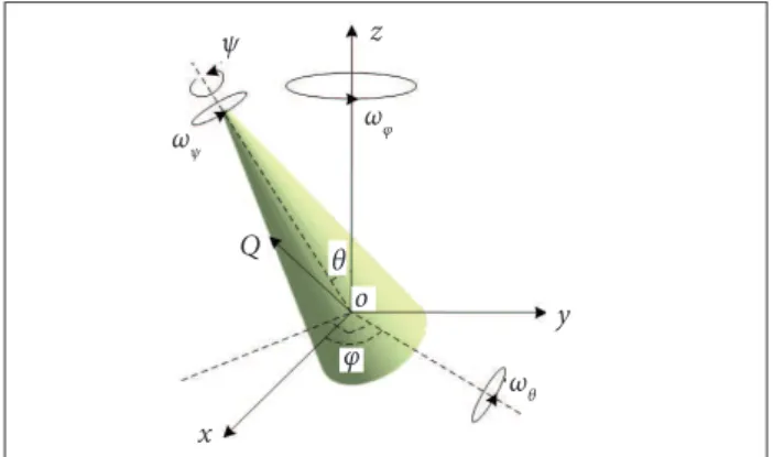
he recognition of cone target’s micro-motion of nutation, precession, and spinning is considered in this paper. he micro-motion model of the cone target is shown in Fig. 1.
where: c is speed of light; f is the wave frequency; j is
√–1; σi is the electromagnetic scattering coeicient of the ith
scattering point; Tp is the pulse width; fcis the carrier frequency; γ is the frequency modulation slope; tm is the slow time;
Q
x
z
y
ωθ θ
ωφ
φ o ωψ
ψ
Each micro-motion can be decomposed into three parts: the coning of the coning-shat, the nutation of the nutation-shat, and the spinning of the spinning-shat. Considering the mass center of the cone as the origin, the radar coordinate system is established with the coning-shat as the z axis, the initial nutation-shat as the x axis, and the y axis is established by right-hand screw rule. ConsideringRconi(t) is the Euler rotation matrix (Xu et al. 2012) when time is t, the arbitrary point Q on the cone target can be expressed as rQ in the body coordinate system. In the radar coordinate system, it can be expressed as:
Considering φ as coning angle, θ as nutation angle, and Ψ
as spinning angle, then Rconi(t) in Eq. 2 can be expressed as:
ˆ ˆ
ˆ
(1)
(2)
Since the cone target is a rotational symmetric object and the motion of the rotational symmetric object around the symmetry axis has no efect on the electromagnetic scattering, the change of the spinning angle Ψ in electromagnetic scattering analysis can be neglected. Generally, considering that Ψ = 0°, Eq. 3 can be simpliied as:
scattering source in the ISAR image plane. By applying the high-frequency scattering theory, when the electromagnetic wave is on the stationary cone target, the backscattering is mainly composed of the cone node A and cone bottoms B
and C, which are the cross points of the incident plane and
the edge of the cone bottom (Huang et al. 2005). However, the
cross points of the incident surface and the cone bottom edge are sliding because of the diferent kinds of spatial cone target’s micro-motion. hen it is called cone bottom slip-type scattering center (Ma et al. 2011). Without considering cross
range scaling, the Doppler axis of the ISAR image is scattering source Doppler frequency shit, and the range axis of the ISAR is the projection distance of the scattering source in radar observation direction. Considering that ζ and η are
the unit direction vector of the Doppler axis and range axis, respectively, the projection vector of the cone node scattering
A and the cone bottom slip-type scattering B and C in the
imaging plane can be expressed as:
where: fd_k and lk (k = A, B, C) are the Doppler frequency
shits of the corresponding scattering source and its projection on the distance image, respectively. he derivation procedure of the concrete expression is presented as follows.
he Euler angles of diferent micro-motion forms are set as follows:
• Nutation: considering coning angular rate is ωΨ, initial
coning angle is φ0, initial nutation angle is θ0, swing
amplitude is θs, swing angular rate is ws, and initial
swing phase is θs0, then the coning angle φ and the
nutation angle θ of the nutation model can be expressed as:
• Precession: when the nutation angle is constant, the nutation model can be simpliied as precession model. he nutation angle can be called precession angle, then the coning angle φ and the nutation angle θ of
the precession model can be expressed as:
• Spinning: when the spinning angle and the nutation angle are constant, the nutation model can be simpliied as spinning model. hen the coning angle φ and the
nutation angle θ can be expressed as:
Firstly, the Doppler shit fd_k (k = A, B, C) of the scattering
source under diferent micro-motions is analyzed. he distance between the cone mass center and cone node A is |OA|, and the
coordinate of the cone node A in the body coordinate system
is (0,0,|OA|). By Eq. 2, the coordinate vector of the cone node A in the radar coordinate system can be represented as:
Assuming that α is the angle between radar observation
direction los and the precession axis (z axis), it can be called
radar observation angle. As the radar observation direction
is in the y-z plane, the radar observation direction los can be
expressed as:
(4)
(5)
(7)
(9) (6)
(11)
(12)
(13)
(14) (8)
(10)
PROJECTION TRAJECTORY OF THE CONE TARGET’S STRONG SCATTERING SOURCE
he following is the consideration of the projected trajectory
hen the Doppler frequency shit of the cone node scattering source A can be expressed as:
cone bottom edge slip-type scattering center B is:
where: λ is the wavelength.
By Eqs. 5 and 6, the Doppler frequency shit of the nutation cone target’s cone node scattering can be given as:
where: φ΄ = ωφ and θ΄= ωsθs cos(ωst + θs0).
By Eqs. 7 and 8, the Doppler frequency shit of the precession cone target’s cone node scattering source can be given as:
where: φ΄ = ωφ.
By Eqs. 9 and 10, the Doppler frequency shit of the spinning cone target’s cone node scattering source can be given as:
Next, the Doppler’s theoretical distribution of the cone bottom slip-type scattering source is analyzed. he unit normal vector of the plane which is composed by the radar observation direction los and the cone polar axis can be obtained:
where: i, j, and k are the x axis, y axis, and z axis in the
radar coordinate system, respectively; nOA = rA/|rA|, and the
expression of F is:
hen the cone bottom slip-type strong scattering source
B(C) in the radar coordinate system is:
where: |OO1| is the distance from the cone’s mass center to
the center of the cone bottom; r is the radius of the cone bottom.
hen the Doppler frequency shit of the cone bottom slip-type strong scattering source B(C) is:
By Eqs. 5 and 6, the Doppler frequency shift of the nutation cone target’s cone bottom slip-type strong scattering source is:
By Eqs. 7 and 8, we can obtain the Doppler frequency shit of the precession cone target’s cone bottom slip-type strong scattering source:
(24)
(19) (18) (17) (16)
(20)
(22)
(23)
(21)
hen the unit vector from the cone bottom center O1 to the
(25)
By Eqs. 9 and 10, we can obtain the spinning target’s cone bottom slip-type strong scattering source as follows:
SIMULATION VERIFICATION
To verify the previous analysis, the distribution characteristics of ISAR image of the spatial cone target under different micro-motion forms are simulated. The same structure parameters are used in the simulation of different micro-motion forms, and specific parameters are set as follows: the distance from the mass center to the cone node is |OA| = 1.125 m; the distance from the mass
center to the cone bottom center is |OO1| = 0.375 m; cone
bottom radius is r = 0.252 m; the corner filleted radius of
cone node is r = 0.017 m. The micro-motion parameters
are set as follows: for the nutation, coning angular rate is
ωφ= π rad/s; initial coning angle is φ0 = 0°; initial nutation
angle is θ0 = 20°; amplitude of swing is θs = 10°; the swing
angular rate is ωs = 4π rad/s; initial phase of swing is θs0 = 0°.
For the precession, coning angular rate is ωφ = π rad/s;
initial coning is φ0 = 0°; precession angle is θ = 20°. For
spinning, coning angle is φ = 0° and precession angle is φ = 0°. Assuming that the radar bandwidth is 2 GHz, the
center frequency is 10 GHz, the pulse repetition frequency is 100 kHz, the pulse width is 640 μs, and the target echo is got when α = 45°/135° by electromagnetic simulation.
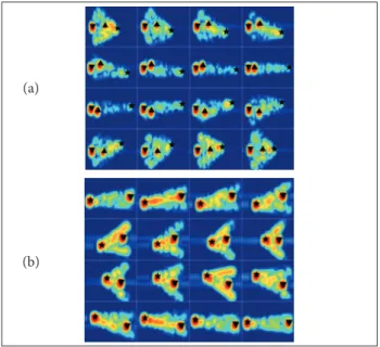
Intercepting an azimuth sampling point of 3,200 from the echo data arbitrarily, 5 × 5 times Fast Fourier Transform (FFT) interpolation into its range and azimuth dimension, setting the extraction interval as 1/8 s, the target’s ISAR image sequence is obtained by the distance-instantaneous Doppler algorithm. To verify the validity of the simulation and the projection trajectory theoretical formula, the strong scattering source distribution in different micro-motion forms is drawn by Eq. 3 to Eq. 5, and the ISAR image sequence is represented in Fig. 3 to Fig. 5.
In the ISAR image sequence from Fig. 3 to Fig. 5, the five-pointed stars represent the theoretical projection position of the cone node scattering A, the inverted triangles represent
the theoretical projection position of the cone bottom scattering B, and the triangles represent the theoretical
projection position of the cone bottom scattering C. It
is not difficult to find that the theoretical value of the scattering source’s projection on the imaging plane is in good agreement with the position of the strong scattering source center in the ISAR image, which shows the accuracy of the imaging algorithm and the projection trajectory formula of the scattering source.
(27)
(28)
(29)
(30)
(31)
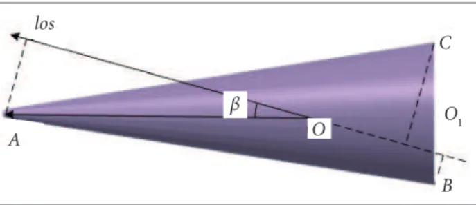
he following continues to consider the analysis of the range axis distribution lk (k = A, B, C) of the scattering source
under diferent micro-motions. For the rotating symmetric cone target, the projection of the strong scattering source in the radar observation direction at any moment is discriminated by the β angle composed by the radar observation direction
los and the cone polar axis OA. By Fig. 2, the projection of the
cone target’s strong scattering source in the range proiles can be expressed as:
where β in Eq. 28 to Eq. 30 can be obtained by cosine
theorem:
Substituting Eq. 5 to Eq. 10 into Eq. 28 to Eq. 30, we can get the scattering sources distribution in the range axis under the corresponding micro-motion.
Substituting Eq. 17 to Eq. 19, Eq. 25 to Eq. 27 and Eq. 28 to Eq. 30 into Eq. 11 to Eq. 13, we can get the projection trajectory of the cone node scattering source A and the cone bottom
slip-type scattering sources B and C.
Figure 2. The strong scattering source’s projection on the
radar observation direction.
C
A
los
B O1 O
Figure 5. The ISAR sequences of the spinning cone target. (a) Radar observation angle is 45°; (b) Radar observation angle is 135°.
Figure 3. The ISAR sequences of the nutation cone target.
(a) Radar observation angle is 45°; (b) Radar observation angle is 135°.
Figure 4. The ISAR sequences of the precession cone
target. (a) Radar observation angle is 45°; (b) Radar observation angle is 135°.
(a) (a)
(a)
(b) (b)
(b)
RECOGNITION FEATURE EXTRACTION
ESTABLISH RECOGNITION FEATURE
Because the ISAR image sequence is a collection of range-instantaneous Doppler distribution extracted from the discrete time points, it is difficult to give a direct visualization of the continuous distribution of the projection
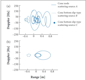
trajectory of each scattering source on the imaging plane. According to Eq. 11 to Eq. 13, the projection trajectory of the strong scattering source on the imaging plane is shown in Figs. 6 and 7. The projection trajectory of the spinning cone target’s strong scattering source on the image plane is a point distribution, because scattering source’s projection on the image plane is constant, which is no longer given in the paper.
According to the previous analysis, there is a big diference in the projection trajectory of the cone target’s strong scattering source under diferent kinds of micro-motion on the imaging plane. For the same cone target model, according to Eq. 11 to Eq. 13, the characteristics of the projection trajectory under the micro-motion parameters and radar observation angle parameters as shown in Table 1 are analyzed.
Parameter Nutation Precession Spinning
fspinning (Hz) 0.5 : 0.1 : 3 0.5 : 0.1 : 3 0.5 : 0.1 : 3
fcone (Hz) 0.5 : 0.1 : 3 0.5 : 0.1 : 3 θ0 (°) 5 : 1 : 25 5 : 1 : 25 θs (°) 5 : 1 : 15
fs (Hz) 0.5 : 0.1 : 3 Radar observation
angle (°) 10 : 5 : 170 10 : 5 : 170 10 : 5 : 170
Table 1. The setting of the micro-motion parameter and
Figure 7. The projection track of the precession cone target’s strong scattering sources on the imaging plane. (a) Radar observation angle is 45°; (b) Radar observation angle is 135°.
Figure 6. The projection trajectory of the nutation cone target’s
strong scattering sources on the imaging plane. (a) Radar observation angle is 45°; (b) Radar observation angle is 135°.
-0.5 0 0.5 1
-250 -200 -150 -100 -50 0 50 100 150 200 250
-0.45 -0.4 -0.35 -20
0 20
-1 -0.8 -0.6 -0.4 -0.2 0 0.2 -250 -200 -150 -100 -50 0 50 100 150 200 250 –1 –0.6 0 –0.35 –0.4 –0.45 –20 0 20 0.5 1 –0.5 –0.2 0.2 –250 –150 –50 50 150 250 250 150 50 –50 –150 –250 D o p p le r [H z] D o p p le r [H z] Range [m] Cone node
s c a t t e r i n g s o u r c e A
C o n e b o t t o m s l i p - t y p e s c a t t e r i n g s o u r c e B
C o n e b o t t o m s l i p - t y p e s c a t t e r i n g s o u r c e C
-0.6 -0.4 -0.2 0 0.2 0.4 0.6 0.8 1 -250 -200 -150 -100 -50 0 50 100 150 200 250 Range/m Doppler/Hz
cone node scattering source A cone bottom slip-type scattering source B cone bottom slip-type scattering source C
0 -100 -50 -150 -200 -250 50 100 150 200 250 Doppler/Hz
-0.46 -0.44 -0.42 -0.4 -0.38 -10
0 10
-1 -0.8 -0.6 -0.4 -0.2 0 0.2 -250 -200 -150 -100 -50 0 50 100 150 200 250 Doppler /Hz 0 -100 -50 -150 -200 -250 50 100 150 200 250
-1 -0.8 -0.6 -0.4 -0.2 0 0.2
Range/m
Cone node
scattering source A
Cone bottom slip-type
scattering source B
Cone bottom slip-type
scattering source C
–250 –150 –50 50 150 250 250 150 50 –50 –150 –250 –0.4 10 0
–10 –0.44 –0.4
0 0.4 0.8
D o p p le r [H z] D o p p le r [H z]
–1 –0.6 –0.2 0.2
Range [m]
(a)
(a) (b)
(b)
According to parameters set in Table 1, about 134,562,714
igures of cone target’s strong scattering sources projection track can be obtained. Ater summing up, we ind that each strong scattering source of the projection trajectory of the nutation cone target has at least two cross points (except for the coning frequency, which is an integral multiple of the swing frequency, or the swing frequency, which is an integral multiple of the
coning frequency). he projection trajectory of each scattering source of the precession target has at most one cross point. he projection trajectory of the spinning target is point distribution, then its Doppler frequency shit is 0 Hz. According to this, we can introduce the recognition criterion that identiies the spinning by Doppler threshold and recognizes the nutation and precession by the cross points number of the scattering source projection trajectory.
In the recognition of micro-motion, the CLEAN algorithm (Caner 2012) can be used to extract the coordinate information of the peak value of the image to get the coordinate information of the point trace. he scattering intensity of the strong scattering source is not always strong under all conditions; under some radar observation angle, the scattering intensity of the cone node strong scattering source may be weak, such as the ISAR images in the second row of Fig. 3a. he scattering intensity of the cone node strong scattering source is weak. It is hard to extract cone node strong scattering source by the CLEAN algorithm, but the cone node strong scattering source is located in the cone node and can be manually extracted by the position of the pointed cone in the ISAR image’s cone contour. hen, the Doppler domain value of the strong scattering source on the imaging plane should be judged. If it is smaller than the set threshold, its corresponding micro-motion form is considered spinning. Otherwise, it is precession or nutation. hen a line segment set is established through connecting the strong scattering sources among adjacent ISAR image sequences; the number of cross points is counted by judging whether line segments intersect. But sometimes the projection trajectories of the different scattering sources overlap, as show in Fig. 8, which has a certain impact on the number of cross points statistics. In addition, single ISAR image exists in multiple scattering centers, so the projection of multiple scattering sources at the adjacent time needs to be related. herefore, it is necessary to separate the projected trajectory of each scattering source. In this paper, the projection trajectory of the cone target’s strong scattering source on the imaging plane is interpreted as the track of target tracking. he target tracking technique is applied to extract the projection trajectory of each scattering source in the ISAR image sequence.
INTERACTING MULTIPLE MODEL KALMAN FILTER
-0.6 -0.4 -0.2 0 0.2 0.4 0.6 0.8 1 -250 -200 -150 -100 -50 0 50 100 150 200 250 Rang/m Doppler/Hz
cone node scattering source A cone bottom slip-type scattering source B con sli -type scattering source C
0 -100 -50 -150 -200 -250 50 100 150 200 250
-0.6 -0.4 -0.2 0 0.2 0.4 0.6 0.8 1
-0.8 -0.6 -0.4 -0.2 0 0.2 0.4 0.6 0.8 1 -250 -200 -150 -100 -50 0 50 100 150 200 250 Dopp ler/Hz 0 -100 -50 -150 -200 -250 50 100 150 200 250 Rang/m cone node scattering source A cone bottom slip-type scattering source B cone bottom slip-type scattering source C
-0.6 -0.4 -0.2 0 0.2 0.4 0.6 0.8
–250 –150 –50 50 150 250 D o p p le r [H z]
–0.4 0 0.4 0.8
Range [m] –250 –150 –50 50 150 250 D o p p le r [H z]
–0.4 0 0.4 0.8
Cone node
scattering source A
Cone bottom slip-type
scattering source B
Cone bottom slip-type
scattering source C
(a)
(b)
and then the motion state of the current and future track is estimated according to the existing points (Shao et al. 2012;
Li et al. 2013). From the previous analysis, the geometric shape
of the cone target’s scattering source on the imaging plane is complex and has the characteristics of spiral, sharp turn and so on. In this case, the Interacting Multiple Model Kalman Filter (IMMKF) algorithm is introduced to predict the target’s track. The algorithm uses multiple motion models to match the tracking target motion mode. At each moment, a certain model is assumed to be valid; the ilter’s initial condition, which matches the certain model, is obtained by mixing all ilters’ estimated states at the previous time. Finally, updating the mode probability by likelihood function of model matching, the state estimation is gained by combining all ilters’ corrected estimated states (Cao and Wen 2010; Deng et al. 2005). In order
to further improve the tracking accuracy, the double-observation points are used to track the distance dimension and Doppler dimension, respectively. he recursive process of the IMMKF algorithmis shown in Fig. 9.
ESTIMATION OF CROSS POINTS NUMBER
Ater extracting and separating the projection point trace of the precession cone target or the nutation cone target in the imaging plane, the intersection can be obtained by judging whether the scattering source’s projection trajectory crosses itself. Cross points only occur between adjacent line segments, and the computing speed would be slowed down by the unnecessary intersection judgement between the far apart segments. he imaging plane is divided into several small facets, only to determine whether there is cross point among the segments in the same facet. When there are many observation points, the cross points based on the face element group are more eicient. Figure 10 gives the low chart of micro-motion recognition of spatial cone target based on ISAR image sequences.
RESULTS
Firstly, the feasibility of recognition feature extraction is veriied. We take the cone target’s cross point of the nutation, precession and spinning, whose radar observation angle is 135°, as an example. Assuming the ISAR imaging sequence extraction interval is 0.04 s, the signal-to-noise ratio (SNR) is 10 dB; other radar parameters and the micro-motion parameters are the same as in the previous section, and the Doppler threshold is set at 20 Hz, which is used to determine whether the micro-motion is spinning. A Doppler distribution of the diferent micro-motion target’s strong scattering sources in the ISAR imaging sequence is shown in Fig. 11, from which the spinning target can be easily recognized.
hen the nutation target and spinning target is continued to be recognized, the tracking algorithm motion model contains one constant velocity (CV) model and two constant turn (CT) models, whose angular rate parameters are ± 6°/s separately. he tracking results by the double observation points are shown in Figs. 12 and 13.
Judging the cross points of the line segments set which is constituted by each scattering source projection point trace in Figs 12 and 13, the number of the projection trajectory’s cross points of both the scattering source A and the scattering source B under nutation is two, and the number of the projection
trajectory’s cross points of both the scattering source A and the
scattering source B under precession is zero, which is consistent
with the recognition criteria already mentioned in which the projection trajectory of each scattering source of the nutation cone target has at least two cross points and the projection trajectory of each scattering source of the precession target has at
Figure 8. The projection trajectory of the nutation cone target and
precession cone target’s strong scattering sources on the imaging plane when the radar observation angle is 70°.(a) Nutation cone target; (b) Precession cone target.
Input intersection Kalman filter Combinatorial output Model probability change
-1 -0.8 -0.6 -0.4 -200 -100 0 100 200 Doppler/Hz 0 -100 -50 -150 -200 -250 50 100 150 200 250
-1 -0.8 -0.6 -0.4
Rang/m
theory distrbution of scattering source A point trace extraction association data
-0.2 -0.1 0 0.1 0.2 0.3 0.4 -200 -100 0 100 200 Doppler/Hz 0 -100 -200 100 200 -0.1
-0.2 0 0.1
Rang/m 0.2 0.3 0.4
theory distrbution of scattering source B point trace extraction association data
–200 –100 0 100 200 D o p p le r [H z]
–0.1 0 0.1 0.2 0.3 0.4
Range [m] –0.2 –200 –100 0 100 200 D o p p le r [H z]
–1 –0.8 –0.6 –0.4
Theory distribution of scattering source A
Theory distribution of scattering source B
Point trace extraction
Association data
-1.2 -1 -0.8 -0.6 -0.4 -0.2 -200 -100 0 100 200 Doppler/ Hz 0 -100 -200 100 200
-1 -0.8 -0.6 -0.4
Rang/m
-1.2 -0.2
theory distrbution of scattering source A point trace extraction association data
-0.2 -0.1 0 0.1 0.2 0.3 -100 -50 0 50 100 Doppler/Hz 0 -50 50 100
-0.1 0 0.1 0.2 0.3
Rang/m -100
theory distrbution of scattering source B point trace extraction association data
–100 –50 0 50 100 D o p p le r [H z]
–0.1 0 0.1 0.2 0.3
Range [m] –200 –100 0 100 200 D o p p le r [H z]
–1.2 –1 –0.8 –0.6 –0.4 –0.2
Theory distribution of scattering source A
Theory distribution of scattering source B
Point trace extraction
Association data (a)
(b)
Echo
Gabor transform
Gabor transform ∑
..
.
..
.
Gabor transform Range profile sequenceISAR Sequence
CLEAN algorithm
Coordinates IMMKF
Track of each scattering source Doppler threslhold
Spin ≥ 2
≤ 1
Cross point number Precession Nutation T im e s am p lin g Bigger Smaller
Figure 10. The low chart of micro-motion recognition of spatial cone target based on ISAR image sequences.
0 5 10 15 20 25 30 35 40 45 50
-150 -100 -50 0 50 100 150 Doppler/Hz 0 -50 50 100 10
0 30 40 50
-100 150 -150 20 frame index Frame index D o p p le r [H z] Spin Precession Nutation Threshold 5 0 5 0 0 –5 0 –100 –150 100 150 40 30 20 10 0
Figure 12. The theoretical, extracted and association results
of the projection trajectory of the nutation cone target’s strong scattering sources on the imaging plane. (a) Cone node scattering source; (b) Cone bottom slip-type scattering source.
Figure 11. The Doppler distribution of the strong scattering
source’s track under different micro-motions.
most one cross point. his shows that the proposed recognition feature extraction technique in the present paper is feasible.
In order to further verify the performance of the algorithm, without considering the condition that the scattering sources may be occluded by the cone target, the radar observation angle range is set from 120° to 140°. Considering three kinds of targets’ simulation parameters, as shown in Table 2, other parameters are still the same as above; the target recognition rate of the target under diferent SNRs is shown in Fig. 14.
From Fig. 14, we find that nutation target has always maintained a high recognition rate. With the increase of
Figure 13. The theoretical, extracted and association results
Parameter Nutation Precession Spinning
fspinning (Hz) 0.5 : 0.5 : 3 0.5 : 0.5 : 3 0.5 : 0.5 : 3
fconning (Hz) 0.5 : 0.5 : 3 0.5 : 0.5 : 3
θ0 (°) 5 : 5 : 25 5 : 5 : 25 5 : 5 : 25
θs (°) 5 : 5 : 15 fs (Hz) 0.5 : 0.5 : 3 Radar observation
angle(°) 120 : 5 : 140 120 : 5 : 140 120 : 5 : 140 SNR (dB) −10 : 2 : 16 −10 : 2 : 16 −10 : 2 : 16
Table 2. The setting of the micro-motion parameter and
radar parameter.
the SNR, precession target and spinning target irst increase and then keep stable. his is due to the high level of noise when the SNR is very low, and the location of the extracted scattering source has a large randomness, then the Doppler
-5 0 5 10 15
100
80
60
40
20
rate of micro-motion recognition/%
SNR/dB
Nutation
Precession
Spin
SNR [dB]
R
at
e o
f mi
cr
o-mo
ti
o
n
r
ec
o
g
ni
ti
o
n [%]
100
80
60
40
20 –5 0 5
10 15
Figure 14. The rate of micro-motion recognition under
different SNRs.
Caner O (2012) Inverse synthetic aperture radar imaging with MATLAB algorithms. New York: John Wiley & Sons.
Cao J, Wen RQ (2010) IMM-UPF algorithm in maneuvering target tracking research. Computer Engineering and Applications 46(28):240-243. doi: 10.3778/j.issn.1002-8331.2010.28.068
Deng XL, Xie JY, Ni HW (2005) Interacting Multiple Model Algorithm with the Unscented Particle Filter (UPF). Chin J Aeronaut 18(4):366-371. doi: 10.1016/S1000-9361(11)60257-4
Guan YS, Zuo QS, Liu HW (2011a) Micro-Doppler signature based cone-shaped target recognition. Chinese Journal of Radio Science 26(2):209-215. doi: 10.13443/j.cjors.2011.02.028
Guan YS, Zuo QS, Liu HW, Du L, Li Y (2011b) Micro-motion characteristic analysis and recognition of cone-shaped targets. Journal of Xidian University 38(2):105-111. doi: 10.3969/j.issn.1001-2400.2011.02.019
frequency shit value of the spinning target’s extracted point trace exceeds the threshold, and the precession target’s cross points increase. Thus, in low SNR, spinning target and precession target are identiied as nutation target, and nutation target is still recognized as nutation target. When the SNR is big enough to afect the scattering center extraction, spin targets and precession targets are accurately identiied. At the same time, it can be found that all kinds of target recognition rates are more than 90% when the SNR is higher than 6 dB, which shows that the proposed algorithm has a good performance of micro-motion recognition in the case of high SNR.
CONCLUSION
Obtaining the micro-motion form of the cone target is the precondition to extract the characteristic parameters of the spatial target. In this paper, a method of extracting feature difference through the ISAR image sequence is proposed to distinguish the micro-motion form of the cone target. Electromagnetic simulation verifies the correctness of the projection trajectory formula of the strong scattering sources in the imaging plane under diferent micro-motion forms. It also illustrates, respectively, the feasibility of the identiication of the spinning target by using Doppler threshold and the recognition of the nutation target and precession target by utilizing the number of the intersection points of the scattering source projection trajectory. Finally, a simulation experiment is carried out to prove the validity of the proposed classiication method.
REFERENCES
Han X, Du L, Liu H W, Shao CY (2013) Classiication of micro-motion form of space cone-shaped objects based on time-frequency distribution. J Syst Eng Electron 35(4):684-691. doi: 10.3969/ j.issn.1001-506X.2013.04.02
Huang PK, Yin HC, Xu XJ (2005) Radar target characteristic. Beijiing: Publishing House of Electronics Industry.
Li F, Jiu B, Shao CY, Liu HW (2013) Curve tracking based parameter estimation of micro-motion. Chinese Journal of Radio Science 28(2):278-284. doi:10.13443/j.cjors.2013.02.024
Ma L, Liu J, Wang T (2011) Micro-Doppler characteristics of sliding-type scattering center on rotationally symmetric target. Scientia Sinica 41(5):1957-1967. doi: 10.1007/s11432-011-4254-3
Shao CY, Du L, Li F, Liu HW (2012) Micro-Doppler extraction from space cone target based on multiple target tracking. Journal of Electronics & Information Technology 34(12):2972-2977. doi: 10.3724/SP.J.1146.2012.00656
Wang T, Wang XS, Chang YL, Liu J, Xiao S (2010a) Estimation of precession parameters and generation of ISAR images of ballistic missile targets. IEEE Trans Aero Electron Syst 46(4):1983-1995. doi: 10.1109/TAES.2010.5595608
Wang ZL, Yan FX, He F, Zhu J (2010b) Missile target automatic recognition from its decoys based on image time-series. Pattern Recogn 43(6):2157-2164. doi: 10.1016/j.patcog.2009.12.016
Xu SK, Liu JH, Wei XZ, Li X, Guo GR (2012) Wideband electromagnetic characteristics modeling and analysis of missile targets in ballistic midcourse. Sci China Technol Sci 55(6):1655-1666. doi: 10.1007/ s11431-012-4864-z
Xu SK, Liu JH, Yuan XY, Lu J (2015) Two dimensional geometric feature inversion method for midcourse target based on ISAR image. Journal of Electronics & Information Technology 37(2):339-345. doi: 10.11999/JEIT140338
Zhou WX (2011) BMD radar target recognition technology. Beijing: Publishing House of Electronics Industry.