ABSTRACT: Performance indexes obtained in idealized simulated scenarios are the primary source of data for evaluating different target tracking algorithms in most researches presented in the literature. Despite the convenience of simulation, ultimate evaluation of a tracking algorithm must be made in real scenarios. Unfortunately, real radar measurements as well as accurate aircraft position, necessary for calculating tracking errors, are not easily available. In this paper, we present an evaluation of the well-known Interacting Multiple-Model with Probabilistic Data Association Filtering algorithm using data obtained from a light inspection of a Brazilian Air Force ground-based long-range surveillance radar. The presented results show that, in this scenario the Interacting Multiple-Model with Probabilistic Data Association Filtering algorithm performance using real data is worse compared to simulation. Statistical properties of the real radar measurements are also investigated, and some evidence is found that embedded noise is not well modeled as perfectly white.
KEYWORDS: Radar tracking, State estimation, Data simulation, Radar data.
Performance Comparison of the
IMMPDAF Algorithm Using Real and
Simulated Radar Measurements
Marcelo Lucena de Souza1, Alberto Gaspar Guimarães2, Ernesto Leite Pinto2
INTRODUCTION
When dealing with simulation for performance evaluation of target tracking algorithms one is faced with the problem of modeling radar measurements and target dynamics. Numerous studies addressing this problem have been published in the literature, and some examples are presented in Bar-Shalom et al. (2001) and Blackman and Popoli (1999).
Radar measurements are oten assumed to be corrupted by additive white Gaussian noise in most simulation setups (Blackman and Popoli 1999), whereas target dynamics are generally emulated with simple kinematic models, such as constant or nearly constant velocity or acceleration models, constant angular rate, or variations and combination of these (Bar-Shalom et al. 2001).
Due to the possibility of real targets exhibiting complex dynamics, target state estimation has been tackled by the multiple-model approach, in which it is assumed that the target can switch between several simpler light models, each one matched to a target mode-of-light (Bar-Shalom et al. 2001).
he Interacting Multiple-Model (IMM) algorithm (Blom and Bar-Shalom 1988) has been widely considered for target state estimation in this context due to its remarkable cost-efectiveness balance (Bar-Shalom et al. 2001). In respect of the origin of the data used for target tracking, it is worth to notice that the IMM algorithm as well as some other multiple-model solutions have been developed assuming unity probability of detection and correct measurement-to-target association.
Some algorithms capable of handling measurement origin uncertainty have been proposed in the literature, such as the
1.Força Aérea Brasileira – Departamento de Controle do Espaço Aéreo – Parque de Material de Eletrônica da Aeronáutica – Rio de Janeiro/RJ – Brazil. 2.Exército Brasileiro – Departamento de Ciência e Tecnologia – Instituto Militar de Engenharia – Rio de Janeiro/RJ – Brazil.
Author for correspondence: Marcelo Lucena de Souza| Força Aérea Brasileira – Departamento de Controle do Espaço Aéreo – Parque de Material de Eletrônica da Aeronáutica | Rua General Gurjão 4 | CEP: 20931-040 – Rio de Janeiro (RJ) – Brazil | Email: [email protected]
Probabilistic Data Association Filter (PDAF) (Bar-Shalom et al. 2009) and its extension to maneuvering targets, the Interacting Multiple-Model with Probabilistic Data Association Filtering (IMMPDAF) (Kirubarajan et al. 1998). Besides the zero-mean white Gaussian measurement noise assumption, these algorithms are also rooted on simplifying assumptions regarding radar performance characteristics and spurious detections, such as constant probability of detection and uniformly-distributed clutter (Bar-Shalom et al. 2011).
Despite being mathematically convenient, such assumptions may be far away from conditions presented by real scenarios of application. herefore it is reasonable to say that only when an algorithm is deployed and evaluated in these scenarios the designer can truly assess its performance. his question has been addressed in some recent researches such as Hess et al. (2014), where eforts have been made to verify the performance of tracking systems in real conditions of inspection lights.
Following this approach, the current paper uses data obtained in a light inspection of a Brazilian Air Force ground-based long-range radar to evaluate the performance of the IMMPDAF algorithm. he results obtained with real measurements are compared to those obtained with simulated data, but the generation of simulated measurements difers from previous studies in the literature. Instead of emulating target dynamics with simple kinematic models, radar measurements are generated by adding white Gaussian noise to the actual target trajectory obtained from the inspection aircrat. he main contribution of this paper is to show that the IMMPDAF can yield larger estimation error in a real environment compared to simulation possibly due to diferent statistical properties of noise in simulated and real environments.
he paper is organized as follows. In the next section, we present basics of target tracking and the IMMPDAF algorithm. Next, data collection and its preparation are described. Aterwards, some numerical results and conclusions are presented.
IMMPDAF AND TARGET TRACKING
BASICS
Under the multiple-model approach, the maneuvering target is modeled as a stochastic dynamic system whose state and observation equations are usually given by:
where: xk, F[Mk], zk and H[Mk] are, respectively, the state vector, state transition matrix, measurement vector and observation matrix at time k. Mk represents the light model in efect at time k and can be any element of the model-set M = {ψj}j=1, being r the number of models. The random sequences {υ [k, Mk]} and {w [k, Mk]} are Gaussian, zero-mean, white and mutually independent. At time k, υ [k, Mk] and w [k, Mk] are random vectors with covariance matrices Q[Mk] and R[Mk], respectively. Given Mk, the values of F[Mk], H[Mk], Q[Mk] and R[Mk] are assumed to be known. The initial state x0is a Gaussian random vector with known mean and covariance matrix. Model transitions are Markovian with probabilities P{Mk= ψj | Mk–1 = ψi} = pij . Both the model-set and transition probabilities pij are assumed constant and known.
Considering measurement uncertainty for handling targets in clutter, association hypotheses are deined to express the choice of a particular measurement-to-track association (Bar-Shalom et al. 2011). In order to avoid searching the entire measurement space to construct measurement-to-track associations, a multidimensional gate, or validation region, is deined. he set of validated measurements (i.e. those that fall inside the validation region or gate) at time k is denoted as Zk = {zk,i}i=1, nk being the number of validations at that time instant. An association hypothesis at time k is deined as Θk = θq, where θq, q ∈ {0 … nk}, is the event in which the q-th measurement was originated from the target of interest, and q = 0 is used for the hypothesis that no measurement came from the target (the target was not detected or its measurement was not validated). he set of all validated measurements up to time k is denoted as Zk = {Zi}k .
he posterior density of the target state vector at time k is written considering all model and association sequences (Bar-Shalom et al. 2011), as follows:
whereLk = ∏l=1 (nl + 1). Mj and Θi represent Mk = ψjand Θk= θi, respectively.
he density in Eq. 3 is a Gaussian mixture with exponentially increasing number of terms, and the evaluation of the a posteriori mean of xk (the Minimum Mean Square Error estimate, referred to as MMSE estimate) cannot be feasibly realized. Numerous sub-optimal algorithms have been proposed in the literature
(1)
(3) (2)
i=1 nk
r
to approximate Eq. 3 and provide good approximations of the MMSE estimate at a feasible computational efort (Blackman and Popoli 1999; Rong Li and Jilkov 2005).
he IMM algorithm has been one of the most successful tools for tracking maneuvering targets without assuming measurement origin uncertainty (Bar-Shalom et al. 2001). On the other hand, the Probabilistic Data Association (PDA) Filter (Bar-Shalom et al. 2009), in particular, handles measurement origin uncertainty for a single light-model by combining the Gaussian mixture representing all measurement associations at time k into a single Gaussian.
he basic idea of the IMMPDAF algorithm is to combine IMM and PDA to track a single maneuvering target in clutter. It irst merges all measurement associations conditioned to the same model at time k into a single Gaussian (PDAF step) and then uses the IMM framework to propagate a Gaussian mixture with r terms.
A detailed description of the IMMPDAF can be found in Bar-Shalom et al. (2011), Kirubarajan et al. (1998) and Sinha et al. (2006). It is worthy to notice that to implement this algorithm in practice some parameters assumed to be known must be chosen by the designer. his is the case of the model-set and the model transition probability matrix. Guidelines for choosing these parameters can be found in Bar-Shalom et al. (2001). Parameter values needed in the measurement-to-track association procedure are the gate probability, i.e. the probability that the true measurement from the target falls into the validation region, and the sensor probability of detection, used in the association probability update. Details about the choice of these parameters can also be found in Bar-Shalom et al. (2011).
DATA COLLECTION
In this section we describe the light inspection data and simulation experiments conducted for evaluating the IMMPDAF algorithm.
FLIGHT INSPECTION
he Brazilian Air Force usually carries out light inspections to evaluate the performance of radar and tracking systems by comparing information from aircrat avionics with those displayed by ground systems. One of these lights was selected for the evaluation presented in this paper. he radar in this inspection is a ground-based long-range surveillance radar,
with antenna rotation period of 10 s. his radar is suitable for air traic control as well as for defense applications.
he light was performed by a Hawker EU-93A aircrat of the Flight Inspection Group (GEIV) of the Brazilian Air Force (DECEA 2015). Its 2-D trajectory obtained onboard from GPS data is depicted in Fig. 1.
Figure 1. Flight inspection 2-D trajectory.
40 80 120 160 200
−100 −60 −20 20 60 100
ξ [NM]
η[NM]
Axis coordinates are given in nautical miles (1 NM = 1,852 m), and the radar was at coordinate (0, 0). he light started at coordinate (80, 0) and comprised a sequence of maneuvers performed by the aircrat. Longitudinal acceleration/deceleration as well as vertical ascending/descending maneuvers (not explicitly shown in the 2-D plot of Fig. 1) have also been executed.
GPS position points were available every second, and the radar produced target measurements every 10 s (antenna rotation period). Consequently, radar data had to be linked to the corresponding GPS position point. his was achieved by analyzing the timestamp of the radar plot and selecting the two nearest GPS position points. These two points were then linearly interpolated to match the radar measurement timestamp.
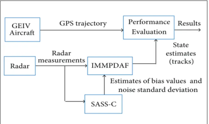
Furthermore, when dealing with real data one has to ensure that biases in measurements are properly corrected to produce zero-mean measurement noise, as it is usually assumed in the evaluation of tracking algorithms. he SASS-C sotware (Zeebroek 2010), developed by EUROCONTROL and licensed to the Brazilian Air Force, was employed to obtain radar measurement bias values that were used in the bias compensation procedure. SASS-C uses trajectory reconstruction algorithms based on Renes et al. (1985) to calculate sensor systematic errors.
Analysis tool (PAA) of SASS-C using real data from a recording of approximately 3 h. his tool calculates diferences between radar measurements and points of the reconstructed trajectory to produce accuracy measures (Zeebroek 2010). hese procedures are summarized in Fig. 2.
NUMERICAL RESULTS
SETUP
he IMMPDAF algorithm was implemented in MATLAB using
the IMMPDAF equations presented in Bar-Shalom et al. (2011).
his implementation had three light models: a nearly-constant
velocity model with process noise standard deviation of 0.1 m/s2,
a discrete Wiener acceleration model with process noise of 3 g,
where g = 9.8 m/s2 is the acceleration of gravity, and a constant
acceleration model (zero process noise). hese are similar to the
models implemented in Bar-Shalom et al. (2001), Heidger and
Mathias (2008) and Kirubarajan et al. (1998). As the state vector
is described in Cartesian coordinates, standard conversion from
polar to Cartesian was applied (Bar-Shalom et al. 2011).
he model transition probability matrix was ixed as: GEIV
Aircraft
Radar IMMPDAF
Performance Evaluation
Radar measurements
Estimates of bias values and noise standard deviation GPS trajectory
State estimates
(tracks) Results
SASS-C
GEIV Aircraft
Radar
IMMPDAF Performance
Evaluation
Radar measurements
Estimates of noise standard deviation GPS trajectory
State estimates
(tracks) Results
SASS-C Measurement
Generation
Simulated measurements
Figure 2. Performance evaluation with real data.
SIMULATION SETUP
For simulation, radar measurements were artificially generated by adding zero-mean white Gaussian noise to the trajectory depicted in Fig. 1. Missed detections observed in the real scenario were considered.
Radar measurements were given in polar coordinates, and noise samples were generated independently in range and
azimuth (Bar-Shalom et al. 2011).
Figure 3 illustrates the simulation setup. It is similar to Fig. 2, differing only that measurements were artificially
generated from aircraft GPS position points. Since no bias
was introduced during measurement generation, there was no need for the IMMPDAF to perform bias correction. he estimates of noise standard deviation were obtained by using SASS-C as above described.
Figure 3. Performance evaluation with simulated data.
where the lines and columns correspond, respectively, to the nearly-constant velocity, discrete Wiener acceleration and constant acceleration models.
Additional choices were the gate probability PG = 0.99 and probability of detection PD = 0.80. his value of gate probability is a common choice (Bar-Shalom et al. 2011), and detection probability of 80% is the minimum required for a primary surveillance radar according to the current Brazilian legislation (DECEA 2014).
The error measure adopted to evaluate the IMMPDAF algorithm was the diference between the aircrat reported position (GPS position) and the position estimate. For radar measurement error analysis, the diference between aircrat GPS position and radar measurements was used.
Since the aircrat GPS generated position reports in geocentric Cartesian coordinates, equations presented in Engel (2005) were applied to transform these reports to a 2-D coordinate system centered on the radar, referred to as local coordinate system. Geocentric aircrat reports were this way transformed to local Cartesian coordinates (ξkGPS, ηkGPS) and local polar coordinates (ρkGPS, θkGPS). For the sake of notational simplicity, the superscript GPS will be suppressed in the following.
IMMPDAF PERFORMANCE WITH REAL AND SIMULATED DATA
To characterize the position error of the IMMPDAF algorithm at time k, diferences in each coordinate were initially computed as:
where ξk and ηk are, respectively, the IMMPDAF estimates for Cartesian coordinates ξ and η at time k.
Estimates of the ensemble averages of the errors at time k for each Cartesian coordinate have been calculated using simulated data as:
and
0 1 0 0 2 0 0 3 0 0 4 0 0 5 0 0 6 0 0
−600 −400 −200 0 200 400 600
k
E
st
im
a
te
s
(m
)
ξ, k η, k and
Figure 4. Estimated averages of IMMPDAF errors from simulation.
where Єξ,k and Єη,k are the errors at time k in coordinates ξ and η, for the ith realization, and N
ENS is the total number of realizations. Figure 4 shows the results obtained for Єξ,k and Єη,k with NENS= 4,000 independent simulations. It can be observed in this igure that the mean of errors in both coordinates varies significantly with time. It is worth noticing that the most signiicant variations may be associated to intense maneuvers, since it has been recognized that Kalman ilter innovations are not zero-mean during these maneuvers (Bar-Shalom et al. 2001).
he results obtained ater averaging over 4,000 independent simulation runs are shown in Fig. 5, where it can be observed that the errors in coordinate η are more intense than those in ξ. his is explained by the fact that the light was carried out mostly eastwards from the radar, where conversion of measurement noise from polar to Cartesian coordinates yielded higher variance in the η axis (Bar-Shalom et al. 2011). Besides, signiicant variations of the standard deviation in both coordinates are exhibited in this igure.
In short, the estimates shown in Figs. 4 and 5 indicate that the IMMPDAF errors are highly non-stationary in both irst- and second-order statistical moments. his is an important fact to be taken into account in the analysis of errors obtained with real data (radar measurements).
(5)
(6)
(8) (7)
(9)
ˆ
ˆ
i i
To gain access to other properties of the IMMPDAF errors with simulated measurements, their standard deviation estimates at time k were computed as:
(10)
0 100 200 300 400 500 600
100 300 500 700 900
k
Estimates [m]
σξ,k ση,k
Figure 5. Estimated standard deviation of IMMPDAF errors from simulation.
It is important to remark that a natural difficulty in comparing performances using real and simulated measurements arises from the fact that real data is usually rare, so a limited number of samples are available and it is not possible to obtain reliable estimates of statistical moments such as those shown in Figs. 4 and 5.
he strategy here adopted to circumvent this diiculty was to verify, through a statistical analysis, if the samples of errors obtained in real conditions of radar operation can be considered as having the same order of magnitude of those obtained with simulated data.
and combined them to form a single normalized error measure
qk deined as:
For the sake of probabilistic modeling it was assumed that q
and q
are independent zero-mean Gaussian random variables with unit variance. Under this assumption, the normalized error amplitude qk has a Rayleigh probability density and mean √π/2.
his is adopted here as a reference probability density for the error amplitude, denoted by pr(.).
So, given a tail probability ∏ arbitrarily set, we are able to evaluate an acceptance interval [0, λ] such that:
Now, with the aim of comparing the IMMPDAF performance subjected to the two sources of measurements, we further deine the variable qR, which is the normalized error measure obtained
with real data. Accordingly, this variable is evaluated using Eq. 13 and error values obtained with real measurements in a similar way of q
and q
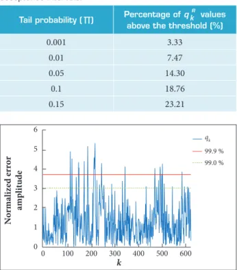
in Eqs. 11 and 12, respectively. he data obtained in 4,000 independent simulation runs and two values for tail probability ∏ (0.01 and 0.001, resulting in λ = 3.03 and 3.71, respectively) have been considered to
plot Fig. 6, which shows the sample function of qR × k and the
thresholds (λ) associated to the acceptance intervals. A large
number of values of qR above these thresholds, i.e. outside the
acceptance interval, may be observed.
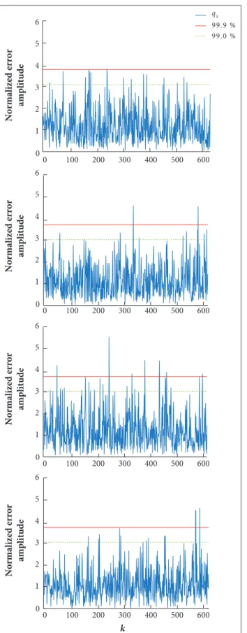
On the other hand, a very diferent behavior is observed in Fig. 7, where samples of normalized errors obtained from four simulation runs are shown. he same thresholds included in the previous igures are used as references. It can be observed that in these cases the thresholds are rarely surpassed, which is an indication of the compliance with the assumed statistical framework.
A quantitative indication of the differences observed in the IMMPDAF performance under the two sources of measurements is given in Table 1, in which the percentages of instantaneous values of qR observed above several threshold (λ)
0 100 200 300 400 500 600
0 1 2 3 4 5 6
k
Normalized error
amplitude
qk
99.9 %
99.0 %
Figure 6. Normalized amplitude of IMMPDAF errors obtained with real measurements.
values are presented, including the two thresholds shown in Fig. 6.
It is shown both in Fig. 6 and Table 1 that the number of instantaneous samplesof qRobtained with radar measurement
data that surpass the chosen thresholds is considerably larger than what should be expected if the IMMPDAF errors with real radar data followed the reference probability distribution.
For further investigation and comparison of the IMMPDAF errors obtained from simulated and real radar data, the RMS position error along with a given (say the ith) simulation run has been calculated as follows:
Table 1. Quantitative evaluation of samples outside acceptance intervals.
(11)
(12)
(13)
(14)
(15)
k
k
real
avg avg
real
k
k k
Tail probability (∏) Percentage of q R
values above the threshold (%)
0.001 3.33
0.01 7.47
0.05 14.30
0.1 18.76
0.15 23.21
k
where N is the number of points in the trajectory. In a
similar way, the RMS error along with the single sample function obtained with real data has been evaluated. It is denoted by
ЄRMS.
he average and standard deviation of the RMS error samples obtained ater 4,000 simulation runs have been calculated and are denoted here as ЄRMS and
RMS, respectively. A comparison
9 9 . 0 % 9 9 . 9 %
qk
0 100 200 300 400 500 600
0 1 2 3 4 5 6
k
Normalized error
amplitude
0 100 200 300 400 500 600
0 1 2 3 4 5 6
Normalized error
amplitude
0 100 200 300 400 500 600
0 1 2 3 4 5 6
Normalized error
amplitude
0 100 200 300 400 500 600
0 1 2 3 4 5 6
Normalized error
amplitude
Figure 7. Samples of normalized error amplitude of IMMPDAF obtained with simulated measurements.
Table 2. IMMPDAF RMS error summary.
It can b e s e e n t h at ЄRMS is 6.56 standard deviations greater than ЄRMS, a signiicant diference of performance. To statistically quantify this diference, we regard the RMS error value as a random variable with irst and second moments ЄRMS and σRMS, respectively. By using the Chebyshev’s inequality, we ind that the probability of observing values of RMS error above ЄRMS is lower than 0.0232.
herefore, this comparison of RMS errors leads us to observe once again that the IMMPDAF performance indexes obtained using real radar data seem not to be statistically consistent with those obtained from simulations.
NOISE ANALYSIS
Radar measurement errors in distance and azimuth were obtained according to:
Measurement type RMS error (m)
Real Єreal = 617.20
Simulated Єavg = 472.78, σavg = 22.01 RMS
RMS RMS
real avg
avg avg
real
where zρ,k and zθ,k are radar measurements at time k in distance and azimuth, respectively.
Considering that the target trajectory was the same for the evaluation of both types of measurements, i.e. simulated and real, we may infer that the difference in IMMPDAF performance using real and simulated data cannot be caused by the target dynamics, but rather resides in the diference of noise characteristics in the two scenarios.
Since bias was compensated, the real measurement noise is assumed to be zero-mean. To further investigate its characteristics, Fig. 8 shows estimates of normalized autocorrelation and cross-correlation functions for radar errors in distance (Єρ,k) and azimuth (Єθ,k), obtained from a single realization of simulation and from real measurements.
Figure 8 shows that the estimates of autocorrelation functions generated from simulated measurements present typical white noise behavior (Figs. 8a and 8c), as expected. It also conirms that simulated measurements in distance
(16)
Figure 8. (a) Normalized autocorrelation of simulated radar distance noise; (b) Normalized autocorrelation of real radar distance noise; (c) Normalized autocorrelation of simulated radar azimuth noise; (d) Normalized autocorrelation of real radar azimuth noise; (e) Normalized cross-correlation of simulated radar noise; (f) Normalized cross-correlation of real radar noise.
(range) and azimuth are uncorrelated (Fig. 8e), as it is usually assumed (Bar-Shalom et al. 2011).
On the other hand, estimates of autocorrelation functions obtained from real measurements (Figs. 8b and 8d) clearly show that the measurement error components at diferent time instants exhibit correlation. So these results suggest that the noise present in real environments would be better modeled as coloured stochastic processes. In Fig. 8f, it is shown that measurement components in polar coordinates present some cross-correlation, in contrast to what is normally assumed in radar tracking algorithms.
CONCLUSION
his paper presented an evaluation of the diference in the IMMPDAF algorithm performance using real and simulated measurements for the same target trajectory. he real measurements were obtained in a light inspection performed by the Brazilian Air Force to evaluate a ground-based long-range surveillance
− 600 − 200 200 600
−0.6 −0.2 0.2 0.6
1 1
Lag
−600 −200 200 600
−0.6 −0.2 0.2 0.6 1
Lag
−600 −200 200 600
−0.6 −0.2 0.2 0.6 1
Lag
−600 −200 200 600
−0.6 −0.2 0.2 0.6 1
Lag
−600 −200 200 600
−0.6 −0.2 0.2 0.6
Lag
1
−600 −200 200 600
−0.6 −0.2 0.2 0.6
Lag
radar. hese radar measurements and GPS position data onboard the aircrat were employed to obtain performance indexes of the IMMPDAF algorithm in a real scenario and compare to those obtained by simulating radar measurements. It was shown that the IMMPDAF performance with real data was worse than that predicted by simulation, and this diference seems to be rooted on diferences between statistical properties of simulated and real measurements. In particular, it was observed that the noise embedded in real radar measurements is not well modeled as perfectly white, contrary to the usual assumption made in simulations. hese results point to the need of more realistic noise modeling in simulation-based performance evaluation of the IMMPDAF algorithm and, as one might infer, in the evaluation of tracking algorithms in general.
ACKNOWLEDGEMENTS
The authors would like to thank the Departamento de Controle do Espaço Aéreo for supporting this research.
(a) (b) (c)
REFERENCES
Bar-Shalom Y, Daum F, Huang J (2009) The probabilistic data association ilter. IEEE Control Syst 29(6):82-100. doi: 10.1109/ MCS.2009.934469
Bar-Shalom Y, Li X, Kirubarajan T (2001) Estimation with applications to tracking and navigation: theory, algorithms and software. Hoboken: Wiley.
Bar-Shalom Y, Willet P, Tian X (2011) Tracking and data fusion: a handbook of algorithms. Storrs: YBS Publishing.
Blackman S, Popoli R (1999)Design and analysis of modern tracking systems. Norwood: Artech House.
Blom HAP, Bar-Shalom Y (1988) The interacting multiple model algorithm for systems with Markovian switching coeficients. IEEE Trans Autom Control 33(8):780-783. doi: 10.1109/9.1299
Departamento de Controle do Espaço Aéreo (2014) Manual Brasileiro de Inspeção em Voo. Brasília: Ministério da Defesa; Comando da Aeronáutica.
Departamento de Controle do Espaço Aéreo (2015) GEIV — Grupo Especial de Inspeção em Voo; [accessed 2015 Dec 23]. http://www. decea.gov.br/?page id=108
Engel A (2005) Coordinate transformation algorithms for the hand-over of targets between POEMS interrogators. Technical report. Brussels: EUROCONTROL.
Heidger R, Mathias A (2008) Multiradar tracking in PHOENIX and its extension to fusion with ADS-B and multilateration. Proceedings of the 5th European Radar Conference; Amsterdam, The Netherlands.
Hess M, Heidger R, Bredemeyer J (2014) Tracker quality monitoring by nondedicated calibration lights. IEEE Aerosp Electron Syst Mag 29(8):10-16. doi: 10.1109/MAES.2014.120028
Kirubarajan T, Bar-Shalom Y, Blair W, Watson G (1998) IMMPDAF for radar management and tracking benchmark with ECM. IEEE Trans Aerosp Electron Syst 34(4):1115-1134. doi: 10.1109/7.722696
Renes JJ, vd Kraan P, Eymann C (1985) Flightpath reconstruction and systematic radar error estimation from multi-radar range-azimuth measurements. Proceedings of the 24th IEEE Conference on Decision and Control. doi: 10.1109/CDC.1985.268714
Rong Li X, Jilkov VP (2005) Survey of maneuvering target tracking. Part V. Multiple-model methods. IEEE Trans Aerosp Electron Syst 41(4):1255-1321. doi: 10.1109/TAES.2005.1561886
Sinha A, Kirubarajan T, Bar-Shalom Y (2006) Tracker and signal processing for the benchmark problem with unresolved targets. IEEE Trans Aerosp Electron Syst 42(1):279-300. doi: 10.1109/ TAES.2006.1603423