Seasonal dependence of the "forecast parameter" based on the EIA characteristics for the prediction of Equatorial Spread F (ESF)

www.ann-geophys.net/26/1751/2008/ © European Geosciences Union 2008

Annales

Geophysicae

Seasonal dependence of the “forecast parameter” based on the EIA

characteristics for the prediction of Equatorial Spread F (ESF)

S. V. Thampi1,*, S. Ravindran1, T. K. Pant1, C. V. Devasia1, and R. Sridharan1

1_{Space Physics Laboratory, Vikram Sarabhai Space Centre, Trivandrum, 695022, India} *_{now at: RISH, Kyoto University, Japan}

Received: 8 October 2007 – Revised: 26 December 2007 – Accepted: 17 January 2008 – Published: 25 June 2008

Abstract. In an earlier study, Thampi et al. (2006) have shown that the strength and asymmetry of Equatorial Ioniza-tion Anomaly (EIA), obtained well ahead of the onset time of Equatorial Spread F (ESF) have a definite role on the subse-quent ESF activity, and a new “forecast parameter” has been identified for the prediction of ESF. This paper presents the observations of EIA strength and asymmetry from the Indian longitudes during the period from August 2005–March 2007. These observations are made using the line of sight Total Electron Content (TEC) measured by a ground-based bea-con receiver located at Trivandrum (8.5◦_{N, 77}◦_{E, 0.5}◦_{N dip} lat) in India. It is seen that the seasonal variability of EIA strength and asymmetry are manifested in the latitudinal gra-dients obtained using the relative TEC measurements. As a consequence, the “forecast parameter” also displays a def-inite seasonal pattern. The seasonal variability of the EIA strength and asymmetry, and the “forecast parameter” are discussed in the present paper and a critical value for has been identified for each month/season. The likely “skill fac-tor” of the new parameter is assessed using the data for a total of 122 days, and it is seen that when the estimated value of the “forecast parameter” exceeds the critical value, the ESF is seen to occur on more than 95% of cases.

Keywords. Ionosphere (Equatorial ionosphere; Ionospheric irregularities; Modeling and forecasting)

1 Introduction

The Equatorial Ionization Anomaly (EIA) and Equatorial Spread F (ESF) are two well known daytime and nighttime processes in the equatorial and low-latitude ionosphere ther-mosphere system. Both these processes have been investi-gated in quite detail through a number of ground and space based instruments (Rishbeth, 2000, and references therein).

Correspondence to:S. V. Thampi (smithathampi@yahoo.com)

Many of these studies showed that the evolution of iono-sphere through the daytime processes like EIA plays an im-portant role in the generation of ESF.

et al., 2004; Manju et al., 2007). All these results conclu-sively established that EIA and ESF are related.

Recently, using the digisonde at Jicamarca and a chain of GPS receivers on the west side of America, it was observed that the seasonal variation in the ESF occurrence is associ-ated with that in the PRE ofE×Bdrift and EIA asymmetry (Lee et al., 2005). It was shown that the largerE×B drift (>20 m/s) and smaller asymmetry (<0.3) provide a prefer-able condition for the development of ESF. It was also re-ported that the seasonal variability of ESF occurrence is asso-ciated with those in the PREE×Bdrift and EIA asymmetry (Lee et al., 2005).

In this context, Thampi et al. (2006) combined the effects of the daytime EIA strength and asymmetry in the time in-terval 16:00–18:45 LT to arrive at a combined parameter (C) that could possibly define the background ionospheric con-ditions, in relation to the occurrence/non-occurrence of ESF. The parameter thus defined was used to “predict” the possi-ble occurrence of post sunset ESF. Using the dataset span-ning from August 2005–January 2006, it was shown thatC

is systematically higher for ESF days. For that limited data set, representing autumnal equinox and winter of low solar activity period, it was shown that a single threshold value of

C=2, clearly separates the ESF days (Thampi et al., 2006). The present paper describes the results using an extended database covering all the four seasons during a low solar ac-tivity period (from August 2005–March 2007), to delineate the seasonal variability of the EIA characteristics and the likely skill factor of the new parameter “C”, which can serve as a forecast parameter for the occurrence/non-occurrence of ESF.

2 Database

The CRABEX receiver located at Trivandrum (8.5◦N, 77◦E, diplat.∼0.5◦N) basically receives the phase coherent signals of 150 and 400 MHz transmitted from the NIMS (Navy Iono-spheric Monitoring System) satellites, and measures the dif-ferential Doppler between them. This is a part of the Coher-ent Radio Beacon ExperimCoher-ent (CRABEX), in which a chain

may not be due to drifting irregularities. However, since we have no means to discriminate the in-situ generated irregu-larities from those drifted into the field of view, the delayed ESF cases have not been considered here, since our aim is to quantify the role of background ionospheric conditions in local generation of ESF.

The TEC data in the time interval 16:00–18:45 IST has been chosen for the estimation of the C-parameter, whereas for studying the general features of the EIA, we have used the data in the time interval 11:30–14:30 IST, (as it is known that EIA is fully developed by 13:00–14:00 LT during low solar activity period (Sastri, 1990)). Owing to the fact that only 3– 4 satellites are being tracked, there are days when we do not have data within this specific time span of 16:00–18:45 IST. Further, it is not possible to get the data exactly at the same time on two consecutive days, since the NIMS satellites are polar orbiting. These are the inherent limitations of our data set itself. In the present study, data from satellite passes with maximum off axis elevation>50◦_{only are selected. For} esti-mating the latitudinal gradients we have used only the part of the data for which the direct elevation angles are>35◦, be-cause the simple secχmapping will not hold good for lower elevation angles. This is the case especially in the equato-rial and low latitude region, where large gradients in electron density exist.

3 Results and discussion

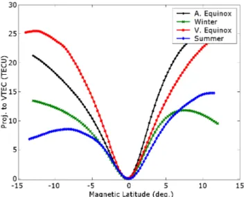
Fig. 1a. The seasonal variability of relative vertical TEC showing the variability in the EIA strength and asymmetry.

Fig. 1b. Latitudinal profiles of TEC in the time interval 11:30– 14:30 IST during September 2005. The thick pink curve shows the monthly mean.

about the dip equator even in the equinoctial months. This can be clearly seen in Fig. 1b, which shows the TEC curves for September 2005. The thick pink curve shows the monthly mean. We can see that EIA asymmetry is present to some ex-tent, with significant day-to-day variability. However, when compared to the solstice months, we can see that the crests are stronger and located farther in latitude, whereas in sol-stice period the winter crest is located closer to the equa-tor. It may be noted that it is this day-to-day variability in the EIA asymmetry, which acts as a proxy for estimat-ing the importance of neutral dynamics in determinestimat-ing the occurrence/non-occurrence of ESF on a given day.

Fig. 2. Variation of EIA strength,SF (top panel) and asymmetry, AF (bottom panel) with day number. The shaded region in the top

panel highlights the cases with similarSF values, with the

occur-rence of ESF (red) on a few days while the other days are without ESF (blue).

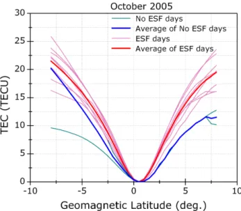
Fig. 3a. Comparison of the latitudinal profiles of relative vertical TEC for ESF and no-ESF days for October 2005.

Fig. 3b.Same as Fig. 3a, but for August 2006.

with the ETWA related convergence at the equator, which in turn determines the magnitude of the vertical winds at the equator.

As mentioned earlier, the previous investigations were mostly focused on relating the EIA strength with the ESF occurrence, mainly using data acquired on one side of EIA. The acquisition of TEC data by CRABEX has the advan-tage of measuring the TEC on both sides of the EIA, which enables to include the effect of asymmetry also. Figure 2 shows the variation of EIA strength, defined asSF= N+S₂ and EIA asymmetry, defined asAF=

N−S

SF

, whereN and

S represent the gradients (TECU/deg.) in the northern and

Fig. 4.Variation ofCwith day number.

southern directions of the dip equator, estimated from rela-tive TEC measurements. It can be seen that there are sev-eral days with ESF, even though theSF values are compar-atively low (shaded region in Fig. 2 (top panel)). Similarly, Fig. 2 (bottom panel) shows that even though the low values ofAF favors the presence of ESF, there are several cases with nearly equal values of AF, with some of them being ESF days, while the others are not. It can be seen that we need to consider the combined effects of EIA strength as well as asymmetry.

Figure 3a–b illustrates this fact more clearly, where the TEC profiles of ESF and no-ESF days of each month is plot-ted with their respective averages (if more than one day data is present). Figure 3a shows the TEC profiles of ESF days (8 days) and no-ESF days (2 days) of October 2005 and their respective averages. It can be clearly seen that the average profile of days when ESF occurred is significantly more sym-metric than that corresponding to the no-ESF days. Figure 3b shows the TEC profiles of ESF day (only 1 day) and no-ESF days (7 days) of August 2006. We can see that the presence of ESF is favored by a strong and symmetric EIA. However, on one day (29 August 2006, shown as dotted curve), in spite of EIA being comparable to that on the ESF day (28 August 2006), the ESF is absent. The cause of this is not clearly understood. However, we can conjecture that one of the pos-sible reasons could be the absence of “seeding perturbation” at F-region altitudes on this day.

Fig. 5a.Monthly variation ofCfor ESF and no-ESF days.

the form

C=q SF

|AF|

=

SF

) N−S

(1)

It has been shown that the combined parameter “C” could ex-plain the presence/absence of ESF on the days with similar values ofSF (Thampi et al., 2006). Figure 4 shows the vari-ation ofCwith day number. It can be seen that even though “C” is systematically higher for ESF days, it has a seasonal variability. It can also be seen that a single threshold value for “C” can be identified for each season, so that when “C” exceeds that particular threshold, ESF is seen to occur on that day. The seasonal dependence of the occurrence of ESF is also evident.

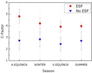
Figure 5a shows the monthly mean values of the C-factor for ESF days (Red) and Non-ESF days (Blue), with the cor-responding standard deviations for each month. It can be seen that the mean values for the non-ESF days are distinctly lower than those for ESF days. Figure 5b shows the seasonal variation of the mean C-factor. Here also, we can see that the C-factor for the ESF days is distinctly higher than those for non-ESF days. The seasonal averages have been estimated using the entire data set from August 2005 to March 2007, representing the low solar activity period.

Another important point, which is to be studied further, is the absence of ESF activity on the three days even though the “C” values are relatively high (Fig. 4). Especially on 3 June, even with a “C” value comparable for the ESF occurrence on equinoctial period, there was no ESF occurrence. Instead, blanketing Es was seen to persist over Trivandrum even dur-ing 19:45 IST (not illustrated). The occurrence of blanketdur-ing Es is also very common during the June–July period in the low-latitude ionosphere over Indian longitudes, in the solar

Fig. 5b.Seasonal variation ofCfor ESF and no-ESF days.

minimum epoch (Devasia, 1976; Devasia et al., 2004). It is known that for estimating the growth rate, the field-line inte-grated ionospheric conductivity should be taken into account (Kelly, 1989; Sultan, 1996). The suppression of ESF activ-ity by the finite E-region conductivactiv-ity at the off-equatorial region is also reported earlier (Kelley et al., 2002; Abdu et al., 2003). The integrated E-region Pederson conductivity can be an important parameter in determining whether the bottom side F-layer will be stable against the R-T instabil-ity (Hanson et al., 1983). This particular aspect would be investigated further using a database of the blanketing Es at the off-equatorial region, the post-sunset height rise at the equator and the subsequent ESF activity. Similarly, on 29 August 2006 and 3 February 2007 also we can see that the C-Factor is comparable to that on near by ESF days, whereas the ESF is absent. These are to be investigated in detail con-sidering other factors like the fraction of bottom-side elec-tron content in the absolute TECs, the presence or absence of “seeding perturbation” etc. on these three days. It should also be noted that all the ESF events observed by the ionosonde could not be included in this study because of the unavailabil-ity of satellite passes at the required time interval on all days. This points out to the requirement of having more number of beacon satellites.

4 Conclusion

reiterates the fact that C-factor can serve as a useful forecast parameter for the occurrence/ non-occurrence of ESF. Acknowledgements. This work was supported by Department of Space, Government of India. One of the authors, Smitha V. Thampi, gratefully acknowledges the financial assistance provided by the In-dian Space Research Organization through a research fellowship. The authors gratefully acknowledge L. Sarala and the other col-leagues at Space Physics Laboratory, for their assistance in the data collection.

Topical Editor M. Pinnock thanks one anonymous referee for her/his help in evaluating this paper.

References

Abdu, M. A., McDougall, J. W., Batista, I. S., Sobral, J. H. A., and Jayachanddran, P. T.: Equatorial evening pre-reversal elec-tric field enhancement and sporadic E layer disruption: A mani-festation of E and F-region coupling, J. Geophys. Res., 108(A6), 1254, doi:10.1029/2002JA009285, 2003.

Anderson, D. N., Reinisch, B., Valladares, C., Chau, J., and Veliz, O.: Forecasting the occurrence of ionospheric scintillation activ-ity in the equatorial ionosphere on a day-to-day basis, J. Atmos. Sol. Terr. Phys., 66, 1567–1570, 2004.

Davies, K.: Recent progress in satellite radiobeacon studies with particular emphasis on the ATS-6 radio beacon experiment, Space Sci. Rev., 25, 357–430, 1980.

Devasia, C. V.: Blanketing sporadic-E characteristics at the equa-torial stations of Trivandrum and Kodaikanal, Indian J. Radio Space Phys., 5, 217–220, 1976.

Devasia, C. V., Jyoti, N., Viswanathan, K. S., Subbarao, K. S. V., Tiwari, D., and Sridharan, R.: On the plausible linkage of ther-mospheric meridional winds with equatorial spread F, J. Atmos. Sol. Terr. Phys., 64, 1–12, 2002.

Devasia, C. V., Jyoti, N., Subbarao, K. S. V., Tiwari, D., Reddi, C. R., and Sridharan, R.: On the role of vertical electron density gradients in the generation of type II irregularities as-sociated with blanketing E S (E Sb) during counter equato-rial electrojet events: A case study, Radio Sci., 39, RS3007, doi:10.1029/2002RS002725, 2004.

Hanson, W. B., Sanatani, S., and Patterson, T. N. L.: Influence of the E-region dynamo on Equatorial spread F, J. Geophys. Res., 88, 3169–3173, 1983.

http://www.ann-geophys.net/23/745/2005/.

Manju G., Devasia, C. V., and Sridharan, R.: On the seasonal vari-ations of the threshold height for the occurrence of equatorial spread F during solar minimum and maximum years, Ann. Geo-phys., 25, 1–7, 2007,

http://www.ann-geophys.net/25/1/2007/.

Maruyama, T.: A diagnostic model for equatorial spread F 1. Model description and applications to the electric field and neutral wind effects, J. Geophys. Res., 93, 14 611–14 622, 1988.

Mendillo, M., Baumgardner, J., Pi. Xiaoquing, Sultan P. J., and Tsunoda, R. T.: Onset conditions for equatorial spread F, J. Geo-phys. Res., 97, 13 865–13 876, 1992.

Mendillo, M., Meriwether, J., and Biondi, M.: Testing the thermo-spheric neutral wind suppression mechanism for day-to-day vari-ability of equatorial spread F, J. Geophys. Res., 106, 3655–3663, 2001.

Raghavarao R., Gupta, S. P., Sekar, R., Narayanan, R., Desai, J. N., Sridharan, R., Babu, V. V., and Sudhakar, V.: Insitu measure-ments of winds electric fields and electron densities at the onset of ESF, J. Atmos. Terr. Phys., 49, 485–492, 1987.

Raghavarao, R., Nageswararao, M., Sastri, J. H., Vyas, G. D., and Sriramarao, M.: Role of equatorial ionization anomaly in the ini-tiation of equatorial spread F, J. Geophys. Res., 93, 5959–5964, 1988.

Raghavarao, R., Hoegy, W. R., Spencer, N. W., and Wharton, L.: Neutral temperature anomaly in the equatorial thermosphere – A source of vertical winds, Geophys. Res. Lett., 20, 1023–1026, 1993.

Raghavarao, R., Suhasini, R., Mayr, H. G., Hoegy, W. R., and Whar-ton, L.: Equatorial Spread F (ESF) and vertical winds, J. Atmos. Sol. Terr. Phys., 61, 607–617, 1999.

Rama Rao P. V. S., Jayachandran, P. T., and Sriram, P.: Ionospheric irregularities, the role of equatorial ionization anomaly, Radio Sci., 32, 1551–1557, 1997.

Rishbeth, H.: The equatorial F-layer: Progress and puzzles, Ann. Geophys., 18, 730–739, 2000,

http://www.ann-geophys.net/18/730/2000/.

Sastri, J. H.: Equatorial anomaly in F region – A review, Indian J. Radio. Space Phys., 19, 225–240, 1990.

Sekar, R. and Raghavarao, R.: Role of vertical winds on the Rayleigh-Taylor mode instabilities of the nighttime equatorial ionosphere, J. Atmos. Terr. Phys., 49, 981–985, 1987.

spread F, J. Geophys. Res., 99, 2205–2213, 1994.

Sridharan, R., Chandra, H., Das, S. R., et al.: Ionization hole cam-paign – a coordinated rocket and ground based study at the onset of equatorial spread F: first results, J. Atmos. Sol. Terr. Phys., 59, 2051–2067, 1997.

Sridharan, R., Pallam Raju, D., and Raghavarao, R.: Precursor to equatorial spread-F in OI 630.0 nm dayglow, Geophys. Res. Lett., 21, 2797–2800, 1994.

Sultan, P. J.: Linear theory and modeling of the Rayleigh-Taylor in-stability leading to the occurrence of equatorial spread F, J. Geo-phys. Res., 101, 26 875–26 891, 1996.

Thampi, S. V., Ravindran, S., Devasia, C. V., Pant, T. K., Sreelatha, P., and Sridharan, R.: First observation of top-side ionization ledges using radio beacon measurements from low earth orbiting satellites, Geophys. Res. Lett., 32, L11104, doi:10.1029/2005GL022883, 2005.

Thampi, S. V., Ravindran, S., Pant, T. K., Devasia, C. V., Sreelatha, P., and Sridharan, R.: Deterministic prediction of post-sunset ESF based on the strength and asymmetry of EIA from ground based TEC measurements – Preliminary results, Geophys. Res. Lett., 33, L13103, doi:10.1029/2006GL026376, 2006.

Valladares, C. E., Basu, S., Groves, K., Hagan, M. P., Hysell, D., Mazzella Jr., A. J., and Sheehan, R. E.: Measurement of the lati-tudinal distribution of TEC during ESF events, J. Geophys. Res., 106, 29 133–29 152, 2001.