Money for nothing?
The net costs of medical training
Sara Ribeirinho Machado
Dissertation submitted in partial fulfilment of requirements for the degree
of Research Master in Economics, at Universidade Nova de Lisboa
Supervisor:
Pedro Pita Barros, FE UNL
Money for nothing?
The net costs of medical training
Abstract
The residency programme is the last stage of medical training, in which residents work under the supervision of a graduated physician. Hosting insti-tutions often claim compensation for the training provided. According to our analysis, given the benefits arising from hosting residents, these institutions should provide medical training without additional compensations.
We jointly consider two effects. Residents spend more resources in the production of health care, but at the same time they are a less expensive substitute to nurses and graduate physicians. We use the fact that residents, in Portugal, are centrally allocated to National Health Service hospitals to treat them as fixed exogenous production factors. The data comes from Portuguese hospitals and primary care centres.
Even though teaching institutions have a higher cost level (2%), cost func-tion estimates point to a small negative marginal impact of the residents in the cost structure of hospitals (-0.02%) and primary care centres (-1%).
Keywords: costs; medical training.
1
Introduction
Graduate Medical Education (GME) is the last stage of medical training, following
the undergraduate studies. The GME can vary between countries, states, or even
across specialties, but all the programmes share some common features. GME is a
two-stage residency program. On the first stage, the resident1
completes a
transi-tional year (or couple of years), carrying out one to three months shifts in several
clinical specialties. Candidates are given daily experience of the different
special-ties, helping them in the ongoing career choice. On the second stage, the resident
is assigned to a specialty programme and advisor, according to some matching
pro-cess, and specializes in a specific medical area. The teaching institution hosting the
programme bears the responsability for the resident’s training.
The problem we address in this paper is whether having residents amongst the
working staff compensates for the effort of training them. If this is not the case, a
monetary transfer should be set, in order to ensure enough GME positions. The cash
transfer could be guaranteed by either the sponsor of the Residency programme2 or
the trainee doctor (resident). In sum, should there be a cash transfer to the hosting
institution? To answer this question, we look at the impact of having a specific
exogenous resource, residents3
, on the institutions’ cost structure. This procedure
makes use of the particular institutional setting to allocate residents to hospitals
(detailed below). If the net cost effect (defined as the cost effect above wage) turns
out to be negligible, there should be no cash transfer at all. On the contrary,
if training residents is an extra cost to the institution, the estimates of the cost
function provide a way to quantify the value of the requested transfer.
The direct impact of residents on costs is the wage paid by the hosting institution.
However, there are other cost effects; the first ones arise from the twofold relationship
between the various types of labor required to provide medical care. The most
obvious is the relation between the supervisor and resident’s work. A physician
spends part of his working hours training and supervising the health care provided by
residents. Nonetheless, he increases the time available to treat patients by assigning
1
The terms resident, intern and trainee doctor will be used interchangeably. It stands for a student which has graduated from Medical School and has engaged a Graduate Medical Education - specialty or general practice - process.
2
In the European case this would be the Ministry of Health, most of the times.
3
other tasks (night shifts, paper work, research assistence) to the trainee doctor.
Savings can also arise from the relation between residents’ and nurses’ labor. A
resident is available to perform a number of routine procedures (sutures, blood
tests, etc.), usually carried out by nurses and/or other technicians. Having residents
performing these tasks doesn’t go without cost. In fact, they spend, on average,
more time and resources (mostly diagnosis procedures and tests) with each patient.
Estimates indicate an excess amount of 9 to 30% of costs of teaching hospitals,
adjusting for differences in the case mix (Rich et al., 1990). Residents are pointed
as the main factor behind the increased level of resource utilization causing the
increase in teaching care costs (Rich et al., 1990; and Kane et al., 2005).
Therefore, the wage paid is only a fraction of the cost of training residents. If
residents are to be considered, the hosting institution changes the choice of the type
of resources and their allocation in the provision of health care, and as a result the
optimal production structure differs between teaching and non-teaching hospitals.
We use data from Portugal, applying a model that is common to standard
grad-uate medical education programmes. Two particular features of the Portuguese
system allow us to isolate the cost effect of residents. The first one is the exogeneity
of the process by which residents are assigned to hosting institutions. The second
is the fact that GME is provided almost free of charge to students, even though
they represent a cost to the provider of care. Should this cost lead to a monetary
transfer to the hosting institution, beyond wage? Or is it the case that residents, a
less expensive resource, are a valuable asset, that leads to efficiency gains? Given
the structural differences in the provision of acute (specialty training) and primary
health care (general practitioner training, in the Portuguese healthcare system),
both cases are treated separately.
Our results indicate that both the hospitals’ and primary centres cost structures
are affected by the presence of residents. The average net cost effect on hospitals is
negative (−11,022e, about 40% of the average yearly wage per intern) and the same
happens at Primary Care Centres. Therefore, the net cost turns out to be a net
benefit. Replication of the approach to other countries and data sets will provide
further knowledge of medical training costs.
The paper is organized as follows: Section 2 provides a brief description of the
3, Graduate Medical Education in Portugal, contains the features of Graduate
Med-ical Education in general, and some important characteristics of the Portuguese
programme; the model is presented in Section 4, followed by the data (Section 5)
and estimation results (Section 6 and 7) in both acute and primary care settings.
Section 8 shows the net cost effects of training. Section 9 briefly reports on an
informal survey on residents’ workload, and Section 10 concludes.
2
Literature review
The analysis of medical training has focused on both funding and efficiency issues.
One of the main topics on Graduate Medical Education is the identification of
di-rect and indidi-rect costs of medical training, since didi-rect costs of education (wages
and teaching hours) are easy to measure, but indirect costs are for the most part
unobservable.
The Indirect Medical Education costs (IME) have been studied by several
au-thors. The study by Anderson et al. (2001) provides an overview of the policy
de-bate around GME. The analysis by Thorpe (1988), Rogowski and Newhouse (1992)
and Dalton and Norton (2001) studies the Medicare GME reimbursement formulae.
Regression analysis was used to estimate the indirect costs, to find whether the
re-imbursement formulae is the most suitable and if it provides the proper incentives
to hosting institutions. The effect of teaching on costs might arise from the higher
level of diagnostic and therapeutic services, extra time to perform routine tasks and
the faculty supervision required by residents, as argued by Blumentahl et al. (1997).
The indirect benefits are not so straightforward to measure. Nonetheless, some of
these authors state that indirect medical education costs seem to be redundant
-hospitals are reimbursed for training costs once by residents and a second time by
the government. Overall, no clear picture about GME emerges and, as Newhouse
and Wilensky (2001) explain in their article, the debate goes on.
The other line of research on GME focuses on the link between teaching
sta-tus4
and efficiency. The paper by Jensen and Morrisey (1986) identifies differences
between the production of teaching and non-teaching hospitals due to the role of
4
residents in the production of health care. Furthermore, there is evidence of a higher
cost level for teaching hospitals (Sloan et al., 1993, and Farsi and Filippini, 2008).
For the last twenty years many authors tried to understand the (in)efficiency issues
behind those cost differences.
The tools most widely applied to cost efficiency analysis are stochastic frontier
(SFA) and data envelopment analysis (DEA).5
A review of the studies conducted
using stochastic frontier analysis is available in Rosko (2004). The authors aim to
measure the inefficiency of US teaching hospitals; Linna and H¨akinnen (2006) do
the same for Finnish hospitals. The paper by Grosskoptf et al. (2001) applies DEA
to a sample of 213 US teaching hospitals.6
The authors conclude that teaching
hospitals could reduce substancially the level of inputs keeping the output level, but
are unable to do so due to ineficciency in the production of health care. The choice
of the most suitable estimation technique depends upon the type of data available
(Jacobs, 2001).
We build on this literature in several ways, detailed below. We use similar
econometric procedures. As it will be clear, the particular way by which residents
are assigned to institutions allows us to follow a specific approach, measuring directly
the teaching costs in a way consistent with economic theory. By doing so, we depart
from most empirical analysis, which use only the information on teaching versus
non-teaching status of the hospital. We are able to identify a small but statistically
significant effect on the costs of hosting institutions.
3
Graduate Medical Education in Portugal
Medical education has two stages. In the first stage, the undergraduate years,
stu-dents acquire a strong theoretical background. The purpose of the second stage,
graduate medical education, is to empower residents with skills that allow them to
become (independent, i.e., responsible for their actions) practitioneers of a specific
medical specialty. Each health system has its own GME plan, but some of the
features are common to all of them.
When a resident is in the first phase of GME, any decision concerning the
pa-5
See Jacobs, Smith and Street (2006) for a discussion on the topic and examples.
6
tient’s medical condition and treatment is subject to the approval of the supervising
physician, who bears the responsability for the treatment. In the United Kingdom
(UK), this stage corresponds to the first year of the Foundation Programme; in
Portugal, to the Common Year Internship.
The final stage of GME lasts from three to six years, depending on the specialty.
The admission process to specialty programmes (specialty or primary care practice
training) relies on the matching between residents and the residency positions issued
by teaching hospitals or medical centres.7
In some countries, such as the US or
the UK, candidates apply to residency programmes offered by teaching hospitals,
and bargain over wage and labour conditions. We expect the wage to account
for the productivity of the resident, presumably lower than the one attained by a
senior physician. There are matching processes8
aiming to optimize the allocation
of residents to the vacancies issued by teaching hospitals.
However, in other countries, teaching institutions do not bargain over candidates
and the wage to be paid. Instead, the National Accreditation Council sets the
num-ber of vacancies and residency programmes available at each teaching institution.
The process of matching residents with positions is based solely on the candidate’s
profile resulting from National Classifying Examinations and undergraduate student
records, thus being exogenous to teaching institutions.
The exogeneity of the matching process is the key assumption for understanding
the cost effect of residents on the production of health care. If teaching institutions
cannot choose the residents, wages and the number and type of positions available,
each resident becomes a fixed factor in the production of health care. We can
measure their impact on the cost structure of the hosting institution using regression
analysis.
The Portuguese GME process is an example of such a system. Medical training
programmes are highly regulated by the Ministry of Health (MoH).9
The demand
7
In order to become a teaching hospital or medical centre, the institution is subject to an accreditation process, having to fulfil a set of prerequisites regarding facilities, services and avail-ability of supervising physicians. In Portugal, the process is coordinated by the National Council of the Resident (CNMI). In the US, the process is lead by the Accreditation Council for Graduate Medical Education (ACGME). The same type of advisory board exists in many other countries.
8
In the US, the matching process is run by the National Resident Match Program for the majority of GME programmes.
9
for residents’ labor, i.e., the list of available positions in training programmes, is
published by the National Council for Medical Residencies (NCMR), with the advice
of the National Council of Physicians, and issued by the MoH. Each institution’s
ability to host residents (how many and for which specialties) is evaluated by the
NCMR, and there’s nothing the hospital or primary care centre can do about it.
Moreover, the wage is fixed by the MoH.
The supply of residents’ labour is also regulated. In Portugal, as well as in
France, in order to access the last stage of medical training, residents sit the National
Classifying Examinations (NCE). Given NCE grades and the undergraduate student
record, the MoH ranks the students. Therefore, the student record determines the
order by which candidates choose (their free of charge) GME programme. The
matching takes place in a predetermined week, one candidate choosing at the time.
When the matching process is over, teaching institutions are informed about the
residents they are to train over the next few years.
Such a system allows to isolate the cost effect of residents. We have a laboratory
to analyse the impact of having a fixed and exogenous number of residents, and
check whether there is a related increase in costs, beyond the wage cost.
4
The Model
We estimate the effect of residents on an institution’s total cost. The estimation
procedure is defined taking into account the particularities of the production
fac-tors involved in medical care. Along with the demand for physical capital inputs
(facilities, beds, laboratories, medical devices, taken as a “composite bundle”), the
provision of health care requires highly specialized labor input, both medical (Lm)
and nursing (Ln). Assume there are three labor inputs able to perform these tasks
- physicians (L1), residents (L2) and nurses (L3). The interaction among these can
be written as:
Lm =L1 +βL2 (1)
Ln =L3+θL2. (2)
The demand for medical labor can be met by both senior physicians and
labor is equivalent. If it was, the parameter β would be equal to one. If residents
are able to perform some of the tasks carried out by physicians (or the same but at
a different pace)10
, the parameter is such that β ∈ (0,1). In any case, the rate at
which one type of labor input substitutes for the other is assumed to be constant.
Residents increase the demand for physicians if not only they cannot replace
doc-tors when providing medical care but also prevent them from doing so (β <0). The
same logic applies to nurse work and the parameter θ. We could also think about
different forms of substitutability, but the main message would go through.11
The goal of an institution hosting residents is to find the best way to allocate
available resources, in order to produce the maximum output (medical care) at
the lowest cost. We focus on cost function analysis. The data available (input
prices, output quantities and total expenditure on the inputs used) is suitable to
estimate the cost function (using several econometric techniques12
) and to check for
the robustness of the results.
Formally, the institution faces the following optimization problem:
min
L1,L3,K
C = 3
X
i=1
wiLi+rK (3)
s.t. G(q1, q2, q3) = F (L1+βL2, L3+θL2, K). (4)
whereC stands for total cost of production,Gis total output,F is the technological
relationship using inputs in the transformation function, L1 denotes senior
physi-cians, L2 denotes residents, L3 stands for nurse staff, K represents other inputs.
Finally, wj denotes average wage for the jth type of labour input and r is the cost
of capital.
One important feature of our model is the exogeneity of L2. The number of
10
According to Folland, Goodman and Stano (2006, pp. 344-349), there is evidence that residents increase medical care production in terms of discharges, even though their contribution is below one could expect, given the higher rate of resource utilization.
11
By writing the interaction equations as
L
m=L1+βf(L2)
L
n=L3+θg(L2),
we can assume different forms for the substitutability pattern. For example, decreasing returns to scale is given byg(L2) =
√
L2. 12
residents is a fixed factor for each institution, with a strictly exogenous price. Both
the number of residents and the wage paid are set by the MoH, as described in the
previous section. In face of that, the institution cannot treat residents as a variable
factor, similar to physicians and nurses. Still, it can adjust the use of variable inputs
to the existence of a higher (or lower) number of residents.
Therefore, the optimization problem can be written as
min
L1,L3,K
L= 3
X
j=1
wjLj +rK +λ(G(q1, q2, q3)−F (L1+βL2, L3+θL2, K)), (5)
incorporating the constraint. By direct application of the envelope theorem in the
optimal solution, the impact of increasing the number of residents is given by
∂L ∂L2
=w2 −βw1−θw3 =ω (6)
whichever the functional form ofG(·) and F(·).
We can follow two approaches to capture the effect described in equation (6).
The first one is to estimate a standard Cobb-Douglas cost function, given by
Ci =ωL2i + ΓXi+εi, (7)
whereωis the coefficient of interest. Its sign, significance and magnitude determine
the relevance of bearing the fixed cost of training a resident for the institution’s cost
structure. The focus is on the average value of the impact. The outputs and control
factors are captured in theXi matrix, and εi is the disturbance term.
The second approach is to estimate directly the substitutability parameters β
and θ. Combining equations (6) and (7), we can estimate the cost net of residents
function (Cei) using
e
Ci =Ci−w2L2i =−β(w1iL2i)−θ(w3iL2i) + ΓXi+δi. (8)
The parameter estimates resulting from this equation can be used to compute
the impact ω in equation (6), together with average wages.13
However, the direct
estimation of the parameters imposes much more structure on the estimates than
13
The value ofw2is not as straightforward as one could expect, since it has to take into account
the previous approach. For the time being we have sidestepped the estimation of
the substitutability parameters, given the inconclusive results arising from the fact
that the parameters have to be taken as equal across all hosting institutions.14
5
Data and Methodology
5.1
Data
The dataset combines information provided by the Ministry of Health (MoH) and
other public institutions. The information gives rise to two separate datasets, one
with the data collected from hospitals (2002 to 200415
), in charge of all the specialty
training programmes, and a single cross-section from Primary Care Centres (2005),
where family or general practitioners are trained. The dataset was constructed with
information provided by the MoH and other public institutions, covering the period
2002-2004 for hospitals and a single cross-section (2005) for primary care centres,
yielding two separate datasets, one for each type of medical training (specialty
(hos-pitals) and GP(primary care centres)). Tables 1 and 2 summarize the main variables
included in the analysis of hospitals’ costs.16
Tables 3 and 4 do the same for primary
care centres data.
There are many hospitals which accept residents for training (75%), but not
so many teaching primary care centres (41%). The teaching status and dimension
are positively correlated.17
Teaching activities have here the meaning of training
14
Details available from the authors upon request. See also the previous working paper version.
15
We take the observations as pooled cross section, without taking into account the possible panel structure of the data. This option is plausible given the changes in management rules, mergers between hospital’s administrative boards and missing observations that ocurred in the period. Panel data estimation procedures didn’t add much information to the results.
16
See Appendix for a full description of the variables’ sources.
17
Table 1: Variable definitions, means and standard errors - hospitals
Definition Sample statistics
All hospitals Teaching hospitals
Mean Min Max Mean Min Max
Physicians 200 7 1112 253 7 1112
(239.54) (253.53)
Residents 43 0 557 57 1 557
(79.14) (87.00)
Nurses 350 34 1598 427 49 1598
(329.40) (339.14)
Total cost 5.31Me 4.15Me 29.0Me 6.65Me 4.44Me 29.0Me
(5.82Me) (6.11Me)
House staff expenditure 2.87Me 0.67Me 14.3Me 3.56Me 2.84Me 14.3Me
(2.89Me) (2.98Me)
Outpatient visits 96095 5259 467734 119909 11616 467734
(92954) (94959)
Discharges 11270 441 47851 13764 441 47851
(9266.77) (9015.41)
EmergencyRoom episodes 84211 0 249420 94171 0 249420
(52759.31) (55602.5)
Case mix 1.07 0.467 2.72 1.08 .467 2.72
(0.352) (0.387)
Beds 307 10 1491 373 10 1491
(267.20) (269.78)
N=202 N=151
Table 2: Variable definitions, means and standard errors - hospitals (contd.)
Code Definition Sample statistics
All TH
hospitals
D SA ==0 if management rules didn’t change 0.233 0.291
(0.424) (0.456)
MedSchool ==1 if Med School 0.213 0.285
(0.410) (0.453)
D 2002 ==1 if year 2002 0.342 0.344
(0.475) (0.477)
D 2003 ==1 if year 2003 0.332 0.331
(0.472) (0.472)
D 2004 ==1 if year 2004 0.327 0.325
(0.470) (0.470)
RHA Alentejo ==1 if Regional Health Administration Alentejo 0.045 0.060
(0.207) (0.238)
RHA Algarve ==1 if Regional Health Administration Algarve 0.030 0.020
(0.170) (0.140)
RHA Centro ==1 if Regional Health Administration Centro 0.351 0.278
(0.479) (0.450)
RHA LVT ==1 if Regional Health Administration LVT 0.297 0.351
(0.458) (0.479)
RHA Norte ==1 if Regional Health Administration Norte 0.277 0.291
(0.449) (0.456)
Level 3 ==1 if Central Hospital 0.233 0.305
(0.424) (0.462)
Level 2 ==1 if District Hospital 0.584 0.623
(0.494) (0.486)
Level 1 ==1 if District - level 1 Hospital 0.183 0.073
(0.388) (0.261)
D 1Q TH beds ==1 if TH and belongs to 1st quartil of beds 0.059 0.079
(0.237) (0.271)
D 2Q TH beds ==1 if TH and belongs to 2nd quartil of beds 0.213 0.285
(0.410) (0.453)
D 3Q TH beds ==1 if TH and belongs to 3rd quartil of beds 0.233 0.311
(0.424) (0.465)
D 4Q TH beds ==1 if TH and belongs to 4th quartil of beds 0.243 0.325
(0.430) (0.470)
R 1Q beds Residents * belongs to 1st quartil of beds 0.416 0.556
(2.091) (2.405)
R 2Q beds Residents * belongs to 2nd quartil of beds 2.970 3.974
(7.438) (8.374)
R 3Q beds Residents * belongs to 3rd quartil of beds 6.960 9.311
(16.911) (19.004)
R 4Q beds Residents * belongs to 4th quartil of beds 32.193 43.066
Table 3: Variable definitions, means and standard errors - Primary Care Centres
Definition Sample statistics
All PCC Teaching PCC
Mean Min Max Mean Min Max
Physicians 22 2 116 35 6 116
(18.24) (18.33)
Residents 2 0 16 4 1 16
(2.68) (2.92)
Nurses 21 2 112 30 8 112
(14.36) (15.53)
Costs 6.87Me 0.65Me 33.06Me 10.08Me 1.84Me 33.06Me
(5.06Me) (5.16Me)
Outpatients 82,026 8,210 414,854 126,447 17,427 414,854
(68,356) (69,489)
SAP episodes 16,253 0 120,811 18,686 0 120,811
(16,260) (19,497)
Exams 1,835 0 48,416 2,328 0 48,416
(5,484) (7,077)
Age≤18 18.8 0.15 27.9 20.0 0.15 27.9
(% of population) (3.4) (3.22)
Age≥65 21.8 0.28 42.7 17.8 0.28 31.9
(% of population) (7.1) (5.04)
Average wage - physicians 56,669e 19,579e 164,380e 50,710e 19,579e 80,700e
(16,805e) (10,078e)
Average wage - nurses 22,065e 12,306e 48,854e 21,158e 12,306e 48,854e
(4,968e) (4,205e)
Teaching PCC 41%
(0.49)
N=292 N=120
Table 4: Variable definitions, means and standard errors - primary care centres (contd.)
Code Definition Sample statistics
All PCC PCC D 3Q Tphys ==1 if TPCC and belongs to 3rd quartil of physicians 0.15 0.37
(0.36) (0.48)
D 4Q Tphys ==1 if TPCC and belongs to 4th quartil of physicians 0.22 0.53
(0.41) (0.50)
R 1Q phys Residents * belongs to 1st quartil of physicians 0.01 0.02
(0.12) (0.18)
R 2Q phys Residents * belongs to 2nd quartil of physicians 0.05 0.13
(0.28) (0.42)
R 3Q phys Residents * belongs to 3rd quartil of physicians 0.41 1.01
(1.23) (1.76)
R 4Q phys Residents * belongs to 4th quartil of physicians 1.13 2.76
(2.59) (3.45) The standard error is reported in parentheses below the mean.
SRS♯ All PCC Teaching PCC SRS♯ All PCC Teaching PCC
Freq Percent Freq Percent Freq Percent Freq Percent Aveiro 19 6.51% 10 8.33% Portalegre 15 5.14% 3 2.50%
Beja 14 4.79% 2 1.67% Porto 17 5.82% 17 14.17%
Braga 15 5.14% 6 5.00% Santar´em 22 7.53% 6 5.00%
Bragan¸ca 12 4.11% 2 1.67% Set´ubal 20 6.85% 10 8.33%
Castelo Branco 11 3.77% 2 1.67% Viana 11 3.77% 6 5.00%
Coimbra 22 7.53% 12 10% Vila Real 16 5.48% 4 3.33%
Guarda 14 4.79% 3 2.50% Viseu 8 2.74% 5 4.17%
Leiria 17 5.82% 11 9.17% Evora´ 15 5.14% 0.83%
Lisboa 44 15.07% 20 16.67%
residents. We are not concerned in this work with classroom teaching and the
extra costs of university hospitals (though we do control for university hospitals in
the estimation procedure). The same happens to the number of residents and the
expenditure level. On average, teaching institutions have higher cost and output
(outpatient visits, inpatient discharges and emergency room episodes) levels. One
needs to account for the asymetric distribution of costs (see Figure 1), when choosing
the most suitable estimation techniques. The variable Residents has the same type
of distribution.
Figure 1: Kernel density
Most of the healthcare centres are located in the Norte, Centro and LVT Regional
Health Administrations.
5.2
Methodology
We apply three alternative estimation methods to equation (7) - OLS, robust
re-gression and stochastic frontier - to control for the characteristics of the data. If the
results turn out to be consistent across the estimations methods, we have a good
es-timate of the impact of the fixed factor residents on the institution’s cost structure.
We have assumed the cost function to be Cobb-Douglas.18
By applying robust regression to the data, we overcome the problem of having
outliers in the data. If we restricted to heteroskedascity-consistent OLS, atypical
observations could affect the accuracy of the expected conditional mean estimates,
18
either over or underestimating the impact of the covariates on the dependent
vari-able. When we resort to robust regression19
, more weight is given to the information
contained on the more typical observations. The iterative process stops when the
estimates converge to some parameter estimate.
On the other hand, when dealing with cost functions, differences between
insti-tutions’ efficiency levels must be taken into account. Two institutions with the same
inputs might have different outputs, and that can be due to inefficiency issues or
to some unobservable random process. When we estimate a stochastic frontier, we
assume the error term of the equation to be composed of two distinct variables, one
of which is the efficiency component. Thus, this estimation procedure removes the
effect of the more inefficient observations on the parameter estimates.20
We used the full set of output variables and controls, and then run a regression
including the variables with significant coefficients, to check for the stability of
pa-rameter estimates.21
The dependent variable is total costs. Along with the number
of residents, we have included a set of variables to capture a size effect. On average,
the impact of training one more resident depends on the size of the institution. As
an example, is is clear to see that the effect on larger hospitals, i.e., the ones
be-longing to the upper quartile of the capacity distribution (number of beds), is most
probably different from the average impact on smaller hospitals.
The set of covariates included in the estimation of cost effects for each dataset
differ. Initial covariates for hospitals’ dataset include output measures - outpatient
visits, inpatient discharges and emergency room episodes (ER) -, the case mix
in-dex to account for disease complexity, and dummy variables for Medical Schools,
the change in management rules22
, the type of hospital: Central hospitals – large
hospitals and with high intensity of technology, District hospitals - medium-sized
hospitals, or District Level 1 hospitals – low differentiation, small units, and the
Regional Health Administration (RHA), along with two yearly dummies (2003 and
19
See in Fox and Long (1990), the chapter by Berk on robust regression (pp. 292-394), for an overview of this estimation method.
20
To estimate the inefficiency term of the stochastic frontier, we have to assume a parametric form for the distribution of the term (exponential or the half-normal distribution). See Kumbhakar and Lovell for further details on cross-section cost frontier models.
21
Full estimates are available in the Appendix. Standard errors and significance levels are as shown in all tables.
22
2004).
The initial model applied to the primary care centres (PCC) dataset includes
output measures - scheduled and non-scheduled visits (termed SAP episodes) - and
the demographic distribution of the population, captured by the percentage of
pop-ulation aged below 18 or above 65 years old, as well as the average wage paid to
both physicians and nurses, and the Sub-Regional Health Administration (SRS).23
6
The training costs (hospitals)
Hospitals’ cost function estimates are shown in Table 5.24
The overall marginal effect of the variable Residents needs to be computed using
parameter estimates of both the number of residents and the interaction terms
in-cluded in the regression (see Section8). For the moment, we can say that, on average,
adding on resident to the house staff increases costs, but relatively large hospitals
are able to save costs by doing so. This effect includes all the necessary adjustments
to host both stages of medical training, foundation and specialty training.
The results are consistent across the three estimation methods. The estimates
are in line with the existing literature on hospital cost functions.25
Outpatient
visits and outpatient discharges are the main cost drivers. ER episodes do not
bear a systematic relationship to cost, as they vary considerably across hospitals.
The larger the hospital (positively correlated with the teaching status), the more
significant is the impact. Since a fraction of them result in admissions to the hospitals
or outpatient visits, part of the cost effect is captured by the former variables.
Central hospitals (taken as the baseline) have higher costs than the other hospitals,
as we would expect. Hospitals facing more complicated cases (proxied by the
case-mix index) are also more costly. The costs vary across the country, being lower in
the north (RHA Norte) than in the southern regions (RHA LVT, the baseline, but
also Alentejo and Algarve).
23
The SRS hosts the residency programmes and determines how are the residents to be allocated to the primary care centres under its jurisdiction. It is also responsible for the funding of these programmes, together with the payment schemes and the budget of each primary care centre.
24
All continuous variables are in the logarithmic form.
25
Table 5: Hospitals - total cost function estimation
OLS Frontier Robust
Variable Full Sign coef Full Sign coef Full Sign coef Residents 0.001∗∗ 0.001∗∗ 0.001∗ 0.001∗∗ 0.001∗ 0.001∗∗
(0.0002) (0.0002) (0.0003) (0.0003) (0.0002) (0.0003)
R 1Q beds -0.012† -0.011† -0.012 -0.011
(0.007) (0.006) (0.007) (0.007)
R 2Q beds -0.001 -0.001 -0.002
(0.003) (0.002) (0.002)
R 3Q beds -0.002∗ -0.002∗ -0.002∗ -0.002∗ -0.002∗ -0.002∗
(0.001) (0.001) (0.001) (0.001) (0.001) (0.001)
Outpatients 0.522∗∗ 0.513∗∗ 0.522∗∗ 0.488∗∗ 0.512∗∗ 0.477∗∗
(0.057) (0.056) (0.049) (0.045) (0.046) (0.041)
Discharges 0.374∗∗ 0.394∗∗ 0.374∗∗ 0.426∗∗ 0.365∗∗ 0.426∗∗
(0.060) (0.057) (0.052) (0.045) (0.049) (0.041)
ER episodes 0.002 0.002 0.004
(0.006) (0.009) (0.008)
Case mix 0.383∗∗ 0.393∗∗ 0.383∗∗ 0.419∗∗ 0.408∗∗ 0.463∗∗
(0.068) (0.057) (0.065) (0.055) (0.061) (0.050)
D SA 0.023 0.023 0.032
(0.038) (0.040) (0.038)
Med School 0.042 0.042 0.075†
(0.051) (0.040) (0.038)
D 2003 0.055 0.063∗ 0.055 0.064∗ 0.033
(0.036) (0.030) (0.034) (0.031) (0.032)
D 2004 0.048 0.058† 0.048 0.061† 0.053 0.046†
(0.037) (0.033) (0.034) (0.032) (0.032) (0.025)
RHA Alentejo 0.107∗ 0.096∗ 0.107 0.069
(0.053) (0.048) (0.068) (0.064)
RHA Algarve 0.111† 0.104† 0.111 0.073
(0.060) (0.055) (0.081) (0.076)
RHA Centro -0.127∗ -0.122∗ -0.127∗∗ -0.158∗∗ -0.192∗∗ -0.216∗∗
(0.052) (0.049) (0.038) (0.035) (0.036) (0.032)
RHA Norte -0.196∗∗ -0.199∗∗ -0.196∗∗ -0.221∗∗ -0.218∗∗ -0.240∗∗
(0.039) (0.036) (0.039) (0.036) (0.037) (0.033)
Level 2 -0.242∗∗ -0.240∗∗ -0.242∗∗ -0.222∗∗ -0.191∗∗ -0.186∗∗
(0.053) (0.045) (0.049) (0.042) (0.046) (0.038)
Level 1 -0.385∗∗ -0.377∗∗ -0.385∗∗ -0.348∗∗ -0.362∗∗ -0.326∗∗
(0.075) (0.064) (0.069) (0.061) (0.065) (0.056)
Constant 8.383∗∗ 8.326∗∗ 8.382∗∗ 8.311 ∗∗ 8.554∗∗ 8.469∗∗
(0.315) (0.296) (1.579) (1.518) (0.242) (0.221)
N 202 202 202 202 202 202
R2
0.9727 0.9724
P-value restr 0.815 0.351 0.190
Significance levels : †: 10% ∗: 5% ∗∗: 1%
7
The training costs (Primary Care Centres)
The Family Practice/GP training programme is similar to the specialty training
pro-grammes. Residents are assigned to a Sub-Regional Health Administration, which
allocates candidates to Primary Care Centres (PCC) according to the availability
of supervising physicians.
The estimation results are shown in Table 6.
Table 6: Primary Care Centres - total cost function estimation
OLS Frontier Robust
Variable Full Sign coef Full Sign coef Full Sign coef R 2Q physicians -0.072∗∗ -0.069∗∗ -0.071∗ -0.076∗ -0.077∗ -0.075∗
(0.022) (0.022) (0.032) (0.031) (0.029) (0.029)
R 3Q physicians -0.004 -0.004 -0.003
(0.008) (0.008) (0.007)
R 4Q physicians 0.007† 0.007∗ 0.007 0.007† 0.007† 0.007†
(0.004) (0.003) (0.004) (0.004) (0.004) (0.004)
Scheduled visits 0.870∗∗ 0.868∗∗ 0.872∗∗ 0.872∗∗ 0.865∗∗ 0.868∗∗
(0.020) (0.019) (0.018) (0.016) (0.016) (0.015)
SAP episodes 0.015∗∗ 0.015∗∗ 0.015∗∗ 0.015∗∗ 0.013∗∗ 0.012∗∗
(0.003) (0.003) (0.002) (0.002) (0.002) (0.002)
Exams 0.001 0.001 0.003
(0.002) (0.003) (0.002)
Age≤18 -0.010 -0.011∗ -0.010∗ -0.011∗∗ -0.006
(0.007) (0.005) (0.005) (0.004) (0.004)
Age≥65 0.001 0.001 0.005∗ 0.006∗∗
(0.003) (0.002) (0.002) (0.002)
w1 0.155∗ 0.163∗ 0.154∗∗ 0.165∗∗ 0.098∗ 0.108∗∗
(0.064) (0.065) (0.046) (0.041) (0.042) (0.038)
w3 0.142∗ 0.148∗ 0.142∗∗ 0.146∗∗ 0.150∗∗ 0.151∗∗
(0.065) (0.063) (0.053) (0.052) (0.048) (0.047)
Constant -10.804∗∗ -10.899∗∗ -10.876∗∗ -11.016∗∗ -10.348∗∗ -10.639∗∗
(0.793) (0.745) (0.765) (0.705) (0.695) (0.626)
(...)
N 292 292 292 292 292 292
R2
0.962 0.9616
P-value restr 0.977 0.846 0.313
Significance levels : †: 10% ∗ : 5% ∗∗: 1%
The standard error is reported in parentheses below parameter estimates. The variable Residents was not included in the estimation due to collinearity.
Once again, the marginal effect of residents on costs varies according to the size
from training one extra resident. The overal marginal effect could be positive or
negative, but we will see in Section 8 that the benefits overcome the costs.
Heteroskedasticity consistent OLS and the stochastic frontier yield very similar
estimates. Most of the effects are also consistent with robust regression estimates.
Scheduled visits are the main cost driver, and average wages have a strong positive
effect on costs. Demographic effects are essentially similar across the models. If we
focus on the conditional mean (OLS) or the efficient frontier, we infer that the higher
the proportion of population aged below 18 years old, the lower the costs. However,
if we constrain the influence of outliers in the data, by using robust regression, the
older the population (higher percentage of population aged above 65 years old), the
higher the costs, which is the same as saying that younger populations are associated
with lower primary care costs. Costs are higher in the capital (Lisbon) than in most
of the SRS.26
8
The net costs of medical training
In this Section, we use the parameter estimates derived so far to compute the average
marginal cost effect of medical training. The first question that arises is whether
teaching residents increases costs, and if it does, by how much. Table 7 provides the
answer to this question.27
Table 7: Teaching costs
Hospitals Primary Care Centres
Average Conf.Int. 95% % Costs Average Conf.Int. 95% % Costs
OLS 10,323me 7,940me 12,706me 2.86% 196me 136me 257me 1.97%
Frontier 10,275me 7,903me 12,648me 2.47% 170me 110me 229me 1.96%
Robust 8,349me 6,376me 10,323me 2.85% 196me 140me 252me 1.59%
On average, a teaching hospital’s expenditure level is more than 2.5% higher
than the cost level of a non-teaching hospital. The same type of effect occurs when
26
See Appendix for the full estimates (Tables 14 and 15). We have omitted SRS parameter estimates to focus on the effects we are most concerned on.
27
we look at primary care centres (around 2%). We derived these results from the
estimates obtained previously.
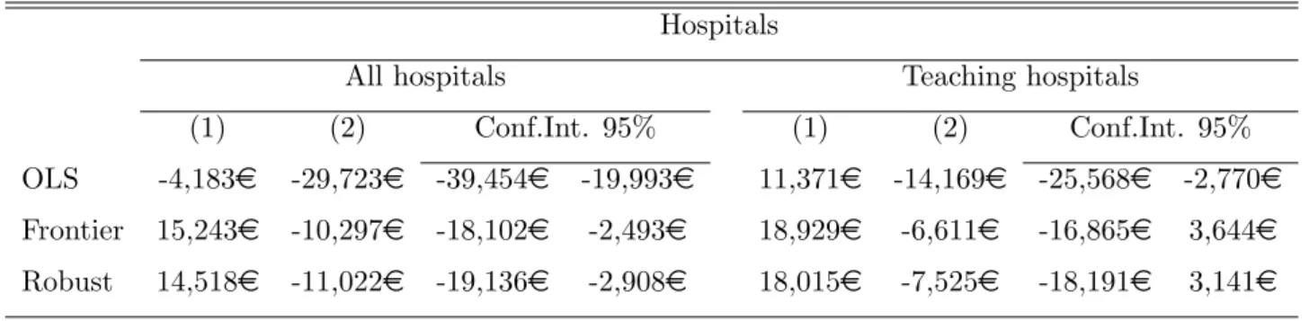
However, we can go one step further. How much does it cost to train one more
resident? What is the net cost (or benefit) of adding one Resident to the house
staff?28
In fact, if an institution trains one more resident, it’s costs will decrease, on
average. Table 8 summarizes the results for each estimation method.
Table 8: Teaching costs - net effect
Hospitals
All hospitals Teaching hospitals
(1) (2) Conf.Int. 95% (1) (2) Conf.Int. 95%
OLS -4,183e -29,723e -39,454e -19,993e 11,371e -14,169e -25,568e -2,770e
Frontier 15,243e -10,297e -18,102e -2,493e 18,929e -6,611e -16,865e 3,644e
Robust 14,518e -11,022e -19,136e -2,908e 18,015e -7,525e -18,191e 3,141e
Primary care centres
All primary care centres Teaching primary care centres
(1) (2) Conf.Int. 95% (1) (2) Conf.Int. 95%
OLS -38,219e -63,759e -80,249e -47,269e 20,670e -4,870e -26,008e 16,269e
Frontier -45,074e -70,614e -88,278e -52,950e 15,849e -9,691e -31,945e 12,563e
Robust -43,858e -69,398e -87,059e -51,737e 17,694e -7,846e -30,209e 14,517e
(1) average marginal effect
(2) net effect = average marginal effect - reference annual wage (resident)
The stochastic frontier and the robust regression yield similar estimates - training
one more Resident decreases hospitals’ costs by 10,000e, on average. The effect is
slightly smaller (7,000e) if we restrict the sample to teaching hospitals. The effect
is higher if we focus on primary care centres. On average, adding one Resident to
the house staff decreases primary care centres’ costs by 1% (Table 9).
28
Table 9: Teaching costs - net effect
Hospitals
All hospitals Teaching hospitals
Net effect (1) (2) (3) Net effect (1) (2) (3)
OLS -29,580e -116.4% -0.105% -0.057% -14,025e -55.5% -0.040% -0.022%
Frontier -10,154e -40.3% -0.036% -0.020% -6,467e -25.9% -0.019% -0.010%
Robust -10,879e -43.2% -0.039% -0.021% -7,382e -29.5% -0.022% -0.012%
Primary Care Centres (PCC)
All PCC Teaching PCC
Net effect (1) (4) (3) Net effect (1) (4) (3)
OLS -63,615 -249.6% -137.5% -0.93% -4,726e -19.1% -10.8% -0.05%
Frontier -70,470 -276.5% -152.3% -1.03% -9,548e -37.9% -21.6% -0.10%
Robust -69,255 -271.7% -149.7% -1.01% -7,703e -30.7% -17.5% -0.08%
(1) percentage of resident’s wage (3) percentage of total costs (2) percentage of house staff expenditure (4) percentage of physician’s wage
Training one more specialist decreases a hospital’s expenditure level by 0.02%
(robust regression parameter estimates), on average. The benefit is lowered to 0.01%
if we restrict to teaching hospitals, due to the proportion of teaching units in the
fourth quartile of the capacity distribution.29
Overall, benefits from training residents seem to occur at both primary care
centres and hospitals, being stronger in the former. At the worst scenario, they
seem to be cost neutral from the point of view of the health care hosting institution.
Residents are being paid below their true productivity, on average (Table 9,
column (1)). Suppose the reference wage of a Resident was increased by 25%
-any institution (hospital or primary care centre) would still face a cost reduction
by training another Resident. Teaching primary care centres benefit less than the
average, since many larger PCC host residents, and in the case of GP training,
smaller institutions benefit more from medical training.
29
9
An alternative view
The quality of data is always a debatable issue and our case is not different. There
is strong variation across health care providers, be it hospitals or primary care
centres. Since our empirical statistical analysis is deeply rooted in the nature of
labor substitution between residents and senior doctors, there is the danger that
our assumptions on this may be leading the results.
To check on the issue, interviews with residents were conducted, where a
descrip-tion of the typical working week of a resident was sought. In particular, we were
interested in identifying time lost by senior doctors on training as well as situations
where residents’ activities replaced those of senior doctors.
According to our sample of residents, their 42 hours schedule can be divided into
five tasks: 12 hours are spent in emergency room shifts (they can devote more than
12 hours to emergency room, but they are paid extra for it); paper work amounts to
10 hours (which would have to be done by senior doctors in the absence of residents),
including writing clinical reports and patient histories; 8 hours are spent with the
supervisor; studying the materials asked by the supervisor takes up to 5 hours;
residents spend 7 hours per week visiting patients and talking to patients’ families.
It is clear residents take up the bureaucratic part of the job, leaving their supervisor
with some extra available time, even taking into account the time they have to spend
with the student.
Residents’ work has some drawbacks. Technically, they are not as good as senior
doctors, above all because of the extra time and resources (mostly diagnosis
pro-cedures) residents spend when treating patients. However, much of this difference
depends on the chosen specialty. Globally, the total effect of residents’ work benefits
the institution, either directly (work) or indirectly (supervisors can spend extra time
providing health care, instead of doing paper work).
By being so, having residents learning at one’s institution is a way of enhancing
the workload distribution among the different types of labour comprised by the
house staff. Therefore, the qualitative information is in line with the econometric
10
Conclusion
Medical training is a lengthy and complex process, involving a number of players
-hospital or primary care centres, physicians, nurses, providers, professors and
stu-dents. The purpose of the paper is to assess the costs and benefits to the institution
that hosts a residency program.
To do so, one has to consider residents as a specific input, able to perform both
physician and nurse staff work. However, the performance is possibly not as efficient
as if it were nurses or physicians to provide care to patients. The presence of this
type of resource may well influence not only the level but also the structure of the
institution’s costs.
In order to address this issue, we estimated the impact of residents on Portuguese
hospitals and primary care centres. The analysis is possible due to the specificities
of the Portuguese Residency programme. The results indicate that providing
med-ical training decreases costs (above the wage of the resident) by a relatively small
amount. This means that claims from hospital and primary care centres’ managers
that teaching consumes resources (time of physicians) are largely compensated for
by the activity with which residentes contribute to the institution. An informal
review of the typical weekly workload of residents seems to corroborate this view.
The effect is stronger in the case of general practitioneer training. Our results have
strong, and important, implications. Given that residents are a fixed exogenous
factor and that organization of labor work at the health care institution adjusts
to take advantage of their presence, there should be no cash transfer to a hosting
institution, either in the form of a subsidy or tuition fee. At most, their wage should
be compensated by transfers from the National Health Service.
A final word to a couple of caveats. Firstly, the quality of data is always an
issue, namely for costs of decision-making units (hospitals or primary care centres).
Second, the short time spam precludes the exploration of the panel data nature of
References
Anderson, G., Greenberg, G., Wynn, B., (2001), “Graduate Medical Education: the policy debate”, Annual Review of Public Health, 22, 35 - 47.
Barros P, de Almeida Sim˜oes J., (2007) Portugal: Health system review. Health Systems in Transition, 2007; 9.
Blumenthal, D, Campbell, E., Weissman, J., (1997) “The social missions of academic health centers” New England Journal of Medicine 337(21), 1550-3.
Dalton, N., (2000), “Revisiting Rogowski and Newhouse on the indirect costs of teaching”, Journal of Health Economics, 19, 1027 - 1046.
Farsi, M., Filippini, M., (2008), “Effects of ownership, subsidization and teaching activities on hospital costs in Switzerland”, Health Economics, 17, 335-350. Folland, S., Goodman, A., Stano, M., (2006),Economics of Health and Health Care,
Prentice Hall; 5th edition.
Fox, S., Long, J.S. (1990),Modern Methods of Data Analysis, Sage Publications. Gouveia, M., Alvim, J., Carvalho, C., Correia, J., Pinto, M., (2006), “Resultados
da Avaliac˜ao dos Hospitais SA”.
Grosskopf, S., Margaritis, D., Valdmanis, V., (2001) “The effects of teaching on hospital productivity”, Socio-Economic Planning Sciences, 35, 189 - 204. Jacobs, R., (2001) “Alternative methods to examine hospital efficiency: data
envel-opment analysis and stochastic frontier analysis”, Health Care Management Science, 4, 103 - 115.
Jacobs, R., Smith, P., and Street, A., (2006), Measuring Efficiency in Health Care - Analytic Techniques and Health Policy, Cambridge University Press.
Jensen, G., Morrisey, M., (1986) “The role of physicians in hospital production”,
The Review of Economics and Statistics, Vol. 68, No
3, pp. 432 - 442.
Kane, R., Bershadsky, B., Weinert, C., Huntington, S., Riley, W., Bershadsky J., Ravdin, J. July (2005), “Estimating the patient care costs of teaching in a teaching hospital”, The American Journal of Medicine, Vol. 118, Issue 7, pp 767 - 772.
Koenig, L., Dobson, S., Siegel, D., Blumenthal, J., Weissman (2003) “Estimating the mission related costs of teaching hospitals”, Health Affairs, 22(6), 136 -148.
Kumbhakar, S. C. and Lovell, C. A. K. (2000): Stochastic Frontier Analysis, Cam-bridge University Press, United Kingdom.
Linna, M. and H¨akkinen, U. (2006), “Reimbursing for the costs of teaching and re-search in finnish hospitals: A stochastic frontier analysis” International Jour-nal of Health Care Finance and Economics, Vol. 6, Number 1, pp 83 - 97.
Newhouse, J., Wilensky, G., (2001) “Paying for Graduate Medical Education: the debate goes on”, Health Affairs, Vol 20, n 2, 136 - 147.
Nicholson, S., Song, D., (2001) “The incentive effects of the Medicare indirect med-ical education policy”, Journal of Health Economics, 20, 909 - 933.
Puig-Junoy, J., Ortun, V., (2003) “Cost Efficiency in Primary Care Contracting: A Stochastic Frontier Cost Function Approach”. UPF Working Paper No. 719. Available at SSRN: http://ssrn.com/abstract=563242.
Rich E.C., Gifford G., Luxemberg M, Dowd B., (1990) “The relationship of house staff experience to the cost and quality of inpatient care.” Journal of the American Medical Association, 263(7):153-71.
Rogowski, J.A., Newhouse, J.P., (1992) “Estimating the indirect costs of teaching”,
Journal of Health Economics, 11, 153 - 171.
Rosko, M., (2004) “Performance of the U.S. teaching hospitals: a panel analysis of cost inefficiency”, Health Care Management Science, 7(1), 7 - 16.
Sloan, F., Feldman, R., Steinwald, B., (1983) “Effects of teaching on hospital costs”,
Journal of Health Economics, 2, 1 - 28.
A
Data sources
Table 10: Data sources
Source Variables
Ministry of Health Physicians, Residents, Nurses
(2002/2005)
Hospitals’ Annual Report Total costs, House staff expenditures,
and Accounts outpatient visits, discharges, emergency room episodes,
(Hospitals - 2002/2004) case-mix index, beds, Medical School, type of hospital
Regional Health Administrations’ Costs, outpatients, SAP episodes,
Tableaux de Bord Exams, age, average wage (physicians and nurses),
(Primary Care Centres - 2005) sub-regional health administration
B
The cost of teaching
We will now focus on the plain old teaching cost effect, which can be done by adding
an indicator variable of the teaching status to the estimated cost function.
Hospitals’ cost function parameter estimates (Table 11) point to a significant
im-pact of teaching on the cost structure. Furthermore, there is a positive relationship
betweem dimension and costs. The effects of the other covariates are similar to the
ones obtained in Section 6.
The results regarding primary care centres show (Table 12) that teaching
insti-tutions have higher costs. However, large teaching instiinsti-tutions can overcome this
negative effect and and up spending less, on average. Once again, the cost function
parameter estimates (Table 12 and 13) are similar to the ones obtained previously
Table 11: Hospitals - total cost function estimation (teaching costs)
OLS Frontier Robust
Variable Full Sign coef Full Sign coef Full Sign coef TH -0.193∗∗ -0.197∗∗ -0.193∗∗ -0.197∗∗ -0.199∗∗ -0.216∗∗
(0.062) (0.061) (0.065) (0.066) (0.062) (0.062)
TH 2Q beds 0.308∗∗ 0.306∗∗ 0.308∗∗ 0.306∗∗ 0.283∗∗ 0.260∗∗
(0.074) (0.071) (0.072) (0.072) (0.068) (0.067)
TH 3Q beds 0.379∗∗ 0.388∗∗ 0.379∗∗ 0.388∗∗ 0.366∗∗ 0.343∗∗
(0.083) (0.076) (0.080) (0.079) (0.075) (0.073)
TH 4Q beds 0.479∗∗ 0.504∗∗ 0.479∗∗ 0.504∗∗ 0.449∗∗ 0.454∗∗
(0.090) (0.087) (0.088) (0.087) (0.083) (0.082)
Outpatients 0.519∗∗ 0.517∗∗ 0.519∗∗ 0.517∗∗ 0.511 ∗∗ 0.500∗∗
(0.052) (0.051) (0.049) (0.048) (0.046) (0.045)
Discharges 0.290∗∗ 0.294∗∗ 0.290∗∗ 0.294∗∗ 0.294∗∗ 0.331∗∗
(0.060) (0.056) (0.052) (0.051) (0.049) (0.048)
ER episodes 0.010 0.010 0.012
(0.006) (0.008) (0.007)
Case mix 0.388∗∗ 0.359∗∗ 0.388∗∗ 0.359∗∗ 0.445∗∗ 0.406∗∗
(0.062) (0.055) (0.060) (0.056) (0.056) (0.053)
D SA -0.003 -0.003 -0.012
(0.038) (0.038) (0.036)
Med School 0.019 0.019 0.063†
(0.047) (0.040) (0.037)
D 2003 0.072∗ 0.071∗ 0.072∗ 0.071∗ 0.050 0.048†
(0.034) (0.029) (0.032) (0.030) (0.031) (0.028)
D 2004 0.061† 0.060† 0.061† 0.060∗ 0.067∗ 0.070∗
(0.034) (0.031) (0.033) (0.031) (0.031) (0.029)
RHA Alentejo 0.068 0.068 0.032
(0.051) (0.067) (0.063)
RHA Algarve 0.154∗∗ 0.144∗∗ 0.154† 0.144† 0.105
(0.055) (0.053) (0.079) (0.079) (0.074)
RHA Centro -0.073 -0.079† -0.073∗ -0.079∗ -0.142∗∗ -0.156∗∗
(0.051) (0.048) (0.037) (0.036) (0.035) (0.033)
RHA Norte -0.155∗∗ -0.163∗∗ -0.155∗∗ -0.163∗∗ -0.167∗∗ -0.194∗∗
(0.037) (0.034) (0.037) (0.036) (0.035) (0.032)
Level 2 -0.291∗∗ -0.279∗∗ -0.291∗∗ -0.279∗∗ -0.231∗∗ -0.231∗∗
(0.048) (0.039) (0.044) (0.039) (0.041) (0.036)
Level 1 -0.446∗∗ -0.434∗∗ -0.446∗∗ -0.434∗∗ -0.415∗∗ -0.409∗∗
(0.065) (0.059) (0.063) (0.059) (0.059) (0.055)
Constant 8.980∗∗ 9.059∗∗ 8.980∗∗ 9.059∗∗ 9.005∗∗ 8.980∗∗
(0.362) (0.362) (1.553) (1.537) (0.284) (0.270)
N 202 202 202 202 202 202
R2
0.9747 0.9743
P-value restr 0.178 0.5311 0.1561
Significance levels : †: 10% ∗: 5% ∗∗: 1%
Table 12: Primary Care Centres- total cost function estimation (teaching costs)
OLS Frontier Robust
Variable Full Sign coef Full Sign coef Full Sign coef Teaching PCC 0.076∗ 0.074∗ 0.075∗ 0.071∗ 0.070∗ 0.069∗
(0.030) (0.030) (0.031) (0.031) (0.029) (0.028)
T 3Q physicians -0.144∗∗ -0.140∗∗ -0.142∗∗ -0.142∗∗ -0.135∗∗ -0.134∗∗
(0.049) (0.048) (0.051) (0.051) (0.047) (0.046)
T 4Q physicians -0.093∗∗ -0.093∗∗ -0.093∗∗ -0.095∗∗ -0.082∗∗ -0.080∗∗
(0.028) (0.028) (0.031) (0.031) (0.029) (0.029)
Outpatients 0.862∗∗ 0.862∗∗ 0.863∗∗ 0.867∗∗ 0.858∗∗ 0.861∗∗
(0.022) (0.021) (0.019) (0.018) (0.017) (0.016)
SAP episodes 0.015∗∗ 0.015∗∗ 0.015∗∗ 0.015∗∗ 0.013∗∗ 0.012∗∗
(0.003) (0.003) (0.002) (0.002) (0.002) (0.002)
Exams 0.001 0.001 0.003
(0.002) (0.003) (0.002)
Age≤18 -0.011 -0.011∗ -0.011∗ -0.011∗∗ -0.006
(0.007) (0.005) (0.005) (0.004) (0.004)
Age≥65 0.001 0.001 0.005† 0.006∗∗
(0.003) (0.003) (0.002) (0.002)
w1 0.166∗ 0.171∗ 0.165∗∗ 0.172∗∗ 0.111∗ 0.120∗∗
(0.065) (0.066) (0.047) (0.042) (0.043) (0.038)
w3 0.148∗ 0.157∗ 0.148∗∗ 0.155∗∗ 0.152∗∗ 0.156∗∗
(0.064) (0.062) (0.052) (0.052) (0.048) (0.048)
Constant -10.886∗∗ -11.010∗∗ -10.950∗∗ -11.126∗∗ -10.441∗∗ -10.734∗∗
(0.797) (0.755) (0.762) (0.703) (0.698) (0.631) Significance levels : †: 10% ∗ : 5% ∗∗: 1%
Table 13: Primary Care Centres- total cost function estimation (teaching costs) SRS variables
OLS Frontier Robust
Variable Full Sign coef Full Sign coef Full Sign coef SRS Aveiro -0.319∗∗ -0.317∗∗ -0.319∗∗ -0.308∗∗ -0.310∗∗ -0.310∗∗
(0.036) (0.032) (0.043) (0.038) (0.040) (0.035)
SRS Beja -0.217∗∗ -0.208∗∗ -0.219∗∗ -0.199∗∗ -0.134∗∗ -0.121∗∗
(0.068) (0.064) (0.053) (0.045) (0.048) (0.042)
SRS Braga -0.181∗∗ -0.179∗∗ -0.181∗∗ -0.170∗∗ -0.171∗∗ -0.196∗∗
(0.043) (0.041) (0.050) (0.047) (0.046) (0.039)
SRS Bragan¸ca -0.111∗ -0.102∗ -0.107† -0.088† -0.106∗ -0.098∗
(0.050) (0.045) (0.058) (0.049) (0.053) (0.045)
SRS Castelo Branco -0.049 -0.048 -0.114∗ -0.095∗
(0.063) (0.056) (0.051) (0.047)
SRS Coimbra -0.104∗∗ -0.098∗∗ -0.103∗ -0.087∗ -0.118∗∗ -0.117∗∗
(0.036) (0.033) (0.042) (0.036) (0.039) (0.033)
SRS Guarda 0.007 0.004 -0.028
(0.057) (0.054) (0.049)
SRS Leiria -0.122∗∗ -0.118∗∗ -0.121∗ -0.107∗ -0.110∗ -0.116∗∗
(0.041) (0.038) (0.047) (0.042) (0.043) (0.039)
SRS Portalegre -0.307∗∗ -0.298∗∗ -0.311∗∗ -0.291∗∗ -0.282∗∗ -0.281∗∗
(0.073) (0.072) (0.052) (0.045) (0.046) (0.042)
SRS Porto -0.189∗∗ -0.187∗∗ -0.189∗∗ -0.181∗∗ -0.172∗∗ -0.192∗∗
(0.048) (0.045) (0.048) (0.045) (0.045) (0.039)
SRS Santar´em -0.373∗∗ -0.363∗∗ -0.372∗∗ -0.354∗∗ -0.374∗∗ -0.363∗∗
(0.039) (0.035) (0.043) (0.036) (0.040) (0.033)
SRS Set´ubal -0.005 -0.005 0.000
(0.036) (0.041) (0.038)
SRS Viana -0.085∗ -0.076† -0.085† -0.088† -0.072†
(0.041) (0.040) (0.051) (0.047) (0.043)
SRS Vila Real -0.158∗∗ -0.155∗∗ -0.157∗∗ -0.143∗∗ -0.154∗∗ -0.159∗∗
(0.046) (0.042) (0.047) (0.041) (0.043) (0.038)
SRS Viseu -0.314∗∗ -0.310∗∗ -0.312∗∗ -0.298∗∗ -0.309∗∗ -0.321∗∗
(0.049) (0.045) (0.063) (0.057) (0.058) (0.051)
SRS ´Evora -0.184∗∗ -0.173∗∗ -0.187∗∗ -0.167∗∗ -0.195∗∗ -0.184∗∗
(0.066) (0.065) (0.049) (0.043) (0.044) (0.040)
N 292 292 292 292 292 292
R2
0.962 0.962
P-value restr 0.974 0.731 0.399
Significance levels : †: 10% ∗ : 5% ∗∗: 1%
C
Estimation results - Primary Care Centres
Table 14: Primary Care Centres - total cost function estimation
OLS Frontier Robust
Variable Full Sign coef Full Sign coef Full Sign coef R 2Q physicians -0.072∗∗ -0.069∗∗ -0.071∗ -0.076∗ -0.077∗ -0.075∗
(0.022) (0.022) (0.032) (0.031) (0.029) (0.029)
R 3Q physicians -0.004 -0.004 -0.003
(0.008) (0.008) (0.007)
R 4Q physicians 0.007† 0.007∗ 0.007 0.007† 0.007† 0.007†
(0.004) (0.003) (0.004) (0.004) (0.004) (0.004)
Outpatients 0.870∗∗ 0.868∗∗ 0.872∗∗ 0.872∗∗ 0.865∗∗ 0.868∗∗
(0.020) (0.019) (0.018) (0.016) (0.016) (0.015)
SAP episodes 0.015∗∗ 0.015∗∗ 0.015∗∗ 0.015∗∗ 0.013∗∗ 0.012∗∗
(0.003) (0.003) (0.002) (0.002) (0.002) (0.002)
Exams 0.001 0.001 0.003
(0.002) (0.003) (0.002)
Age≤18 -0.010 -0.011∗ -0.010∗ -0.011∗∗ -0.006
(0.007) (0.005) (0.005) (0.004) (0.004)
Age≥65 0.001 0.001 0.005∗ 0.006∗∗
(0.003) (0.002) (0.002) (0.002)
w1 0.155∗ 0.163∗ 0.154∗∗ 0.165∗∗ 0.098∗ 0.108∗∗
(0.064) (0.065) (0.046) (0.041) (0.042) (0.038)
w3 0.142∗ 0.148∗ 0.142∗∗ 0.146∗∗ 0.150∗∗ 0.151∗∗
(0.065) (0.063) (0.053) (0.052) (0.048) (0.047)
Constant -10.804∗∗ -10.899∗∗ -10.876∗∗ -11.016∗∗ -10.348∗∗ -10.639∗∗
(0.793) (0.745) (0.765) (0.705) (0.695) (0.626) Significance levels : †: 10% ∗ : 5% ∗∗: 1%
Table 15: Primary Care Centres - total cost function estimation - SRS Variables
OLS Frontier Robust
Variable Full Sign coef Full Sign coef Full Sign coef SRS Aveiro -0.321∗∗ -0.318∗∗ -0.321∗∗ -0.310∗∗ -0.307∗∗ -0.307∗∗
(0.035) (0.032) (0.043) (0.038) (0.039) (0.035)
SRS Beja -0.212∗∗ -0.203∗∗ -0.214∗∗ -0.196∗∗ -0.132∗∗ -0.116∗∗
(0.067) (0.064) (0.053) (0.046) (0.048) (0.042)
SRS Braga -0.190∗∗ -0.186∗∗ -0.190∗∗ -0.178∗∗ -0.175∗∗ -0.198∗∗
(0.043) (0.041) (0.050) (0.047) (0.046) (0.039)
SRS Bragan¸ca -0.108∗ -0.103∗ -0.104† -0.089† -0.105∗ -0.098∗
(0.050) (0.045) (0.057) (0.049) (0.052) (0.045)
SRS Castelo Branco -0.044 -0.044 -0.128∗ -0.106∗
(0.066) (0.056) (0.051) (0.047)
SRS Coimbra -0.105∗∗ -0.103∗∗ -0.104∗ -0.093∗∗ -0.118∗∗ -0.120∗∗
(0.036) (0.032) (0.042) (0.035) (0.039) (0.033)
SRS Guarda 0.009 0.005 -0.029
(0.056) (0.054) (0.049)
SRS Leiria -0.111∗∗ -0.107∗∗ -0.110∗ -0.097∗ -0.097∗ -0.101∗∗
(0.039) (0.037) (0.046) (0.042) (0.042) (0.038)
SRS Portalegre -0.300∗∗ -0.293∗∗ -0.305∗∗ -0.286∗∗ -0.266∗∗ -0.270∗∗
(0.074) (0.072) (0.052) (0.045) (0.046) (0.042)
SRS Porto -0.170∗∗ -0.167∗∗ -0.170∗∗ -0.163∗∗ -0.144∗∗ -0.164∗∗
(0.046) (0.045) (0.047) (0.044) (0.043) (0.038)
SRS Santar´em -0.379∗∗ -0.370∗∗ -0.378∗∗ -0.361∗∗ -0.378∗∗ -0.366∗∗
(0.038) (0.035) (0.043) (0.036) (0.039) (0.033)
SRS Setubal -0.008 -0.008 0.001
(0.036) (0.041) (0.037)
SRS Viana -0.074∗ -0.071∗ -0.074 -0.082† -0.068
(0.035) (0.036) (0.052) (0.048) (0.044)
SRS Vila Real -0.162∗∗ -0.161∗∗ -0.161∗∗ -0.150∗∗ -0.155∗∗ -0.161∗∗
(0.045) (0.042) (0.047) (0.041) (0.043) (0.038)
SRS Viseu -0.324∗∗ -0.324∗∗ -0.322∗∗ -0.314∗∗ -0.311∗∗ -0.326∗∗
(0.049) (0.046) (0.062) (0.057) (0.056) (0.050)
SRS ´Evora -0.187∗∗ -0.175∗∗ -0.191∗∗ -0.170∗∗ -0.204∗∗ -0.191∗∗
(0.066) (0.065) (0.049) (0.044) (0.044) (0.040)
N 292 292 292 292 292 292
R2
0.962 0.9616
P-value restr 0.977 0.846 0.313
Significance levels : †: 10% ∗ : 5% ∗∗: 1%