A WAVELET-BASED MULTIVARIABLE APPROACH FOR FAULT
DETECTION IN DYNAMIC SYSTEMS
Henrique Mohallem Paiva
∗Roberto Kawakami Harrop Galv ˜ao
†Luis Rodrigues
‡ [email protected]∗Department of Flight Control Systems - Empresa Brasileira de Aeron´autica (EMBRAER)
S˜ao Jos´e dos Campos, SP, Brazil.
†Department of Electronic Engineering - Instituto Tecnol ´ogico de Aeron´autica (ITA)
S˜ao Jos´e dos Campos, SP, Brazil.
‡Department of Mechanical and Industrial Engineering - Concordia University, Montreal, QC, Canada.
ABSTRACT
This paper presents a multivariable extension to a recently proposed wavelet-based technique for fault detection. In the original formulation, the Discrete Wavelet Transform is used to carry out dynamic consistency checks between pairs of signals within frequency subbands. For this purpose, mov-ing average models with an integrative term are employed to reproduce the dynamics of the system in each subband un-der consiun-deration. The present work introduces a new archi-tecture allowing the use of subband models with more gen-eral multivariable structures. More specifically, a multivari-able ARX (autoregressive with exogenous input) structure is adopted for each subband model. The proposed technique is illustrated in a case study involving a nonlinear simulation model for an aircraft with a sensor fault. The results show that the multivariable approach outperforms the original for-mulation in terms of residue amplification following the fault onset.
KEYWORDS: Dynamic Systems, Analytical Redundancy, Fault Detection, Wavelets, Multivariable Systems.
Artigo submetido em 11/02/2009 (Id.: 00949) Revisado em 14/04/2009, 22/06/2009
Aceito sob recomendac¸ ˜ao do Editor Associado Prof. Jos ´e Roberto Castilho Piqueira
RESUMO
Uma abordagem multivari ´avel baseada em wavelets para detecc¸˜ao de falhas em sistemas din ˆamicos
Este artigo apresenta uma extens˜ao multivari´avel para uma t´ecnica recentemente proposta de detecc¸˜ao de falhas baseada em wavelets. Na formulac¸˜ao original, a Transformada Wa-velet Discreta ´e utilizada para realizar testes de consistˆencia dinˆamica entre pares de sinais dentro de faixas de freq ¨uˆencia. Para isso, s˜ao empregados modelos do tipo m´edia m´ovel com termo integrativo para reproduzir a dinˆamica do sistema em cada faixa considerada. O presente trabalho introduz uma nova arquitetura, que possibilita o uso de modelos em sub-bandas com estruturas multivari´aveis mais gerais. Mais es-pecificamente, uma estrutura ARX (autoregressiva com en-trada ex´ogena) multivari´avel ´e adotada para cada modelo em sub-bandas. A t´ecnica proposta ´e ilustrada em um estudo de caso envolvendo um modelo de simulac¸˜ao n˜ao-linear para uma aeronave com falha de sensor. Os resultados mostram que a abordagem multivari´avel ´e superior `a formulac¸˜ao ori-ginal em termos de amplificac¸˜ao do res´ıduo ap´os a ocorrˆencia da falha.
(a)
(b)
u
Subband Model Plant
disturbances
y b y
a
y ^ a
Threshold Device
decision subband
residue
Wavelet Filter Bank +
-Fault-detection system Subband
Model
Threshold Device
decision subband
residue
Wavelet Filter Bank +
-Fault-detection system u
Plant
disturbances
y
u ^y
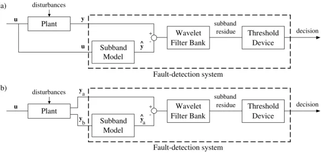
Figure 1: Original wavelet-based analytical redundancy architecture for (a) input-output and (b) output-output consistency checks. The subband model is of the formM(z) = 1−z−1−s
α+βz−1
,s∈Z;α,β ∈R.
1
INTRODUCTION
Prompt fault detection is essential for the improvement of reliability and dependability in complex control systems (Ranganathan et al., 2001), especially for safety-critical ap-plications such as industrial plants (Kallesoe et al., 2006), chemical processes (Simani and Fantuzzi, 2006), automo-tive systems (Fischer et al., 2007) and aircraft (Amato et al., 2006), (Narasimhan and Biswas, 2007).
In this context, the Wavelet Transform (Daubechies, 1992) is a useful tool to detect transient behaviors caused by the on-set of a fault. In (Bhunia and Roy, 2005), a wavelet-based strategy was employed to detect faults in digital CMOS cir-cuits by transient current testing. For this purpose, wavelet coefficients of the current waveform were compared with co-efficients obtained from a fault-free device. In (Zanardelli et al., 2005), the wavelet coefficients of a current signal were used in a classification framework to discriminate between different types of motor faults. In (Kim and Parlos, 2002), a dynamic neural network model was employed to predict the transient response of the system under monitoring. The residues thus generated were then processed by the wavelet transform to compute fault indicators. A combination of model-based residue generation and wavelet processing was also adopted in (Manders and Biswas, 2003), in which a tem-poral causal graph was employed to represent the normal be-havior of the plant.
Most wavelet-related papers in the fault-detection litera-ture exploit two basic approaches, namely: (a) decomposi-tion of a sensor signal containing fault-related informadecomposi-tion (Zanardelli et al., 2005) or (b) decomposition of a residual
signal calculated as the difference between the predictions of a model (or fault-free system) and the actual process output (Bhunia and Roy, 2005; Kim and Parlos, 2002; Manders and Biswas, 2003). A third approach, which was recently pro-posed in (Paiva, Galv˜ao and Yoneyama, 2008), employs the wavelet transform to identify a subband model for the nor-mal behavior of the system, which is then used to generate a residual signal. Such a formulation can be employed to monitor the input-output integrity of the plant (Fig. 1a) or the consistency between two plant outputs (Fig. 1b). A fault is indicated if the filtered difference between plant and model outputs exceeds a pre-defined threshold.
(a)
u y Wavelet
Filter Bank
Threshold Device
decision subband
residue
+ -Subband
Model Wavelet
Filter Bank
Dy
Plant
disturbances
u Du Dy^
Fault-detection system
(b)
u
Plant
disturbances
y b y
a Wavelet Filter Bank
Threshold Device
decision subband
residue
+ -Subband
Model Wavelet
Filter Bank
Dy b Dy
a
^
Dya
Fault-detection system
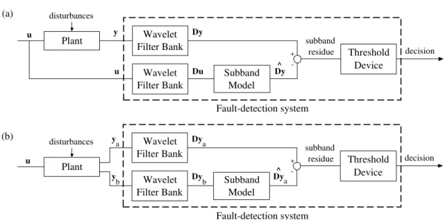
Figure 2: Frequency-Subband Analytical Redundancy Architecture adopted for the multivariable approach. (a) Input-output and (b) output-output consistency check.
structure is adopted for each subband model. Preliminary results obtained with this extension were reported in (Paiva, Galv˜ao and Rodrigues, 2008), where a simplified example involving the linear model of a Boeing 747 aircraft was dis-cussed. In the present work, the effectiveness of the extended technique is demonstrated in a case study involving the non-linear aircraft simulation model ADMIRE (Forssell and Nils-son, 2005), which represents a generic small single-seat fighter aircraft with a delta-canard configuration. A sensor fault is considered for illustration. The fault detection perfor-mance is evaluated under the effect of model uncertainties, sensor dynamics, measurement noise and exogenous distur-bances. The results of the proposed multivariable technique are compared with those obtained by using the original for-mulation presented in (Paiva, Galv˜ao and Yoneyama, 2008).
2
PROPOSED MULTIVARIABLE FAULT
DETECTION TECHNIQUE
In the SISO (single-input, single-output) architecture adopted in (Paiva, Galv˜ao and Yoneyama, 2008) (Fig. 1), the subband model parametersα, β, sare adjusted in order to minimize the norm of the subband residue under normal operation conditions. However, standard identification tech-niques cannot be directly employed because the transmission path between the subband model input (uin Fig. 1a orybin Fig. 1b) and the subband residue involves the wavelet filter bank, which has to be taken into account. To circumvent this problem, an ad-hoc least-squares identification proce-dure was proposed in (Paiva, Galv˜ao and Yoneyama, 2008). In the present paper, a different architecture (Fig. 2) is
adopted in order to facilitate the extension to the MIMO case. In this new architecture, the subband model is placed after the wavelet filter bank.
The remaining of this section will be focused on the input-output scheme (Fig. 2a) for brevity. However, the discussion can be easily extended to the output-output scheme (Fig. 2b) by replacing plant inputuand plant outputyby plant outputs
ybandya, respectively.
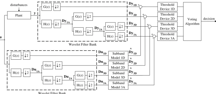
Fig. 3 shows a more detailed representation of the scheme presented in Fig. 2a. Filters H and G indicate the lowpass and highpass filters associated to a particular wavelet, respec-tively.
u
Plant disturbances
y
Wavelet Filter Bank H(z)
G(z)
2 2
H(z) G(z) 2
2
H(z) G(z)
2 2 Du
2A Du
1A
Wavelet Filter Bank H(z)
G(z)
2 2
H(z) G(z) 2
2
H(z) G(z)
2 2
Dy2A
Dy1A decision
Subband Model 1D Subband Model 2D
Subband Model 3D
Subband Model 3A
Threshold Device 3D Threshold Device 2D Threshold Device 1D
Threshold Device 3A
Voting Algorithm
-+ -+ -+ -+
Du1D
Du 2D
Du3D
Du3A
Dy1D
Dy2D
Dy3D
Dy3A
Dy^ 1D
Dy 2D ^
Dy^ 3D
Dy^ 3A
decision
Figure 3: Wavelet-Based Frequency-Subband Analytical Redundancy Scheme
In the wavelet filter bank, the number of filtering iterations leading to a given layer is termed the decomposition level of that layer. In Fig. 3, for example, the filter bank has three decomposition levels. The best decomposition level for fault detection depends on the spectral signature of the fault, as well as the power spectrum density of the input signal and the signal-to-noise ratio of the measurements (Paiva, Galv˜ao and Yoneyama, 2008). If the fault effect has not been previously characterized, all levels should be monitored simultaneously. The outputs of the lowpass and highpass filters are termed approximation and detail, respectively. SubscriptsiA andiD will be used to indicate the approximation and detail at the
i-th decomposition level, respectively. The wavelet coeffi-cientsDuiA(approximation) andDuiD(detail) of the input
signaluat thei-th decomposition level,i >0, are calculated as
DuiA= (↓2) [h∗Du(i−1)A] (1) DuiD= (↓2) [g∗Du(i−1)A] (2)
where (↓ 2) and * denote the downsampling and convolu-tion operaconvolu-tions, andhandgare the discrete-time impulse re-sponses of filters H and G, respectively. The approximation
Du0Aat level 0 is equal to signaluitself. Similar equations
can be used to obtain the wavelet coefficientsDyiA
(approx-imation) andDyiD(detail) of the output signaly.
The configuration adopted for each subband model in Fig. 3 is a multivariable ARX (autoregressive with exogenous
in-put) structure of the form (Ljung, 1999):
ˆ
Dy(k) =
na
X
i=1
AiDyˆ (k−i) + nb
X
i=1
BiDu(k−i),
Ai∈Rp×p, Bi∈Rp×m (3) whereDu(k)∈RmandDyˆ (k)∈Rpcorrespond to the in-put and outin-put of the subband model at time indexk. Since each subband model is intended to represent the plant behav-ior only within a limited frequency band, the ordersnaand
nb can be made small. Matrices Ai, Bi can be identified in order to minimize the 2-norm of the difference between the model predictions Dyˆ and the wavelet coefficientsDy
of the actual plant output. For this purpose, a standard multi-variable least-squares identification method can be employed (Ljung, 1999).
After the identification has been carried out, the threshold for each subband detector can be established on the basis of the subband residue(Dy−Dyˆ )obtained for nominal (fault-free) conditions. In this work, the threshold is set to three times the standard deviation of the residue calculated by us-ing signals u,ydifferent from those employed for identifi-cation.
system under study and the fault effect (Paiva, Galv˜ao and Yoneyama, 2008). In the present work, the overall fault mon-itor declares a fault if any threshold detector is activated. It is worth noting that time resolution decreases as the de-composition is carried out from one level to the next. As a result, longer detection delays may be expected at the final levels of the filter bank. This feature may impose a restric-tion on the maximum number of resolurestric-tion levels that can be employed in the fault monitor.
Summary
In what follows, the algorithm to construct the fault-detection structure presented in Fig. 3 is shortly summarized.
1. Collect signalsuandyto perform the identification of the subband models.
2. Choose wavelet filters H and G and the number of de-composition levels of the wavelet tree.
3. Calculate the wavelet coefficientsDuandDyat each decomposition level.
4. Use an ARX identification procedure (Ljung, 1999) to identify the subband model matrices in Eq. (3).
5. Collect new signalsuandyto establish the thresholds.
6. Calculate, at each decomposition level, the wavelet co-efficientsDuandDyof the new signals, and obtain the corresponding subband model outputDyˆ .
7. Establish the thresholds as a function of the residue
(Dy−Dyˆ ).
The ARX model order could be selected by using tech-niques such as Akaike’s information theoretic criterion (AIC) (Ljung, 1999), Rissanen’s minimum description length (MDL) principle (Ljung, 1999) or generalized cross-validation (GCV) (Sj ¨oberg et al., 1995), (Paiva and Galv˜ao, 2006). Alternatively, the order may be increased, starting from a small value, until the fault detection performance is deemed acceptable. It is worth noting that, as the identifica-tion only concerns the system dynamics within a restricted frequency range, the subband model order can be small as compared to a time-domain ARX representation.
As a general rule, the thresholds should be set to the small-est values that still result in a satisfactory false alarm rate, according to the requirements of the application at hand. If faulty data were available, the thresholds could be chosen to achieve an appropriate trade-off between fault detection and false alarm rates.
3
APPLICATION EXAMPLE
In this section, a case study involving the nonlinear aircraft simulation model ADMIRE (Aero-Data Model In a Research Environment) will be presented.
3.1
System Description
ADMIRE is a generic model of a small single-seat fighter aircraft with a delta-canard configuration. The model is aug-mented with longitudinal and lateral flight control systems to provide stability and handling qualities and contains a rudi-mentary speed controller. The model envelope extends up to Mach 1.2 and altitude of 6 km. A detailed description of this model, as well as the electronic files required for simulation, can be found in (Forssell and Nilsson, 2005).
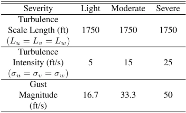
In the present study, turbulence and wind gust models were incorporated in the simulation. The turbulence models fol-low the Dryden form (U.S. Military Specification MIL-F-8785C, 1980). The turbulence scale lengths, turbulence intensities, and gust magnitude were adopted according to (U.S. Military Specification MIL-F-8785C, 1980) in order to simulate light, moderate and severe atmospheric distur-bances, as shown in Table 1.
Table 1: Atmospheric disturbance parameters.
Severity Light Moderate Severe Turbulence
Scale Length (ft) 1750 1750 1750
(Lu=Lv =Lw) Turbulence
Intensity (ft/s) 5 15 25
(σu=σv =σw) Gust
Magnitude 16.7 33.3 50
(ft/s)
ADMIRE contains dynamic models of the rate gyros respon-sible for measuring the body-fixed roll-ratepb, pitch rateqb and yaw-raterb. In this study, zero-mean white noise with standard deviation of 0.2 deg/s was added to the output of each rate gyro. This noise level is realistic for aeronautical sensors, as discussed in (Bacon et al., 2001).
3.2
Simulations
The following sets of simulations were conducted:
A set of fault-free simulations was carried out to identify the subband system models. In each simulation, the aircraft was initially trimmed at straight level. Since the dynamic response of the aircraft varies with the velocity and altitude of operation, twelve points in the envelope (three velocities versus four altitudes) were chosen for trimming: Mach 0.6, 0.9 and 1.2; altitude of 3, 4, 5 and 6 km. For each point, the system was simulated during 20 s under light atmospheric disturbance. In order to enrich the spectral content of the ex-citation signals, small slow-varying augmentation commands were added to the rudder and canard commands generated by the control law. Such augmentation commands consist of a zero-mean square wave with peak-to-peak amplitude of 2.8 deg and frequency of 0.5 Hz. Fig. 4 shows, for a particular simulation, the total rudder and canard commands, as well as the angular rates.
- Threshold definition
A second set of twelve fault-free simulations (one for each point of the envelope) was carried out to establish the thresh-old for each detector. The simulation conditions were similar to those employed in the identification phase, but with differ-ent realizations of atmospheric disturbance and sensor noise.
- Fault simulations
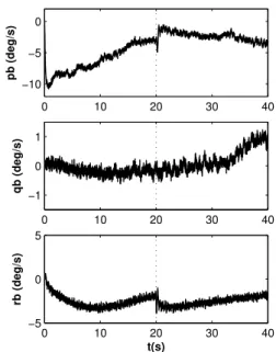
The fault detection problem consisted of detecting a bias of 1.0 deg/s in the yaw rate (rb) gyro. The bias was inserted at t = 20 s in a simulation lasting 40 s. Three different cases were considered:
Case 1 - Straight level:The aircraft was trimmed in straight level at the twelve envelope points specified above. In order to illustrate the robustness of the technique to exogenous dis-turbances, three simulations were carried out for each point, considering different atmospheric disturbance levels (light, moderate and severe). Therefore, a total of 36 simulations were performed. Fig. 5 shows the angular rates obtained in a particular simulation. As can be seen, the fault in therb sensor also induced a change in the behavior ofpb. Such a coupling effect is caused by the closed-loop control system.
Case 2 - Straight level with uncertainties: In order to il-lustrate the robustness of the technique to model uncertain-ties, the system was simulated considering the mass, inertia and center of gravity (CG) uncertainties specified in Table 2. These are the maximum uncertainties that can be used with the ADMIRE model (Forssell and Nilsson, 2005). Each of the 36 simulations described in Case 1 was repeated twice: first with the positive uncertainties in Table 2, and then with the negative ones. Therefore, a total of 72 simulations were carried out.
Case 3 - Altitude Change:In this case, the fault detection
per-Table 2: ADMIRE uncertainty parameters. Parameter Uncertainty
Inertia Ixx ±20 %
Iyy ±5 %
Izz ±8 %
Ixz ±15 %
Mass M ±20 %
CG Position xCG ±0.15 m
yCG ±0.1 m
formance was evaluated during an altitude change manoeu-ver, rather than in straight flight. The airplane was initially trimmed at Mach 1, altitude of 6 km, and then descended to an altitude of 4 km. The system was simulated under light, moderate and severe atmospheric disturbance.
0 10 20 30 40
−10 −5 0
pb (deg/s)
0 10 20 30 40
−1 0 1
qb (deg/s)
0 10 20 30 40
−5 0 5
rb (deg/s)
t(s)
0 5 10 15 20 −2
0 2
drc (deg)
0 5 10 15 20
−2 0 2
dlc (deg)
0 5 10 15 20
−2 0 2
dr (deg)
0 5 10 15 20
−10 0 10
pb (deg/s)
t(s)
0 5 10 15 20
−5 0 5
qb (deg/s)
t(s)
0 5 10 15 20
−5 0 5
rb (deg/s)
t(s)
Figure 4: Angular rates and canard/rudder commands obtained in one of the simulations used for identification. drc, dlc and dr denote the total commands for the right canard, left canard and rudder, respectively. In this particular simulation, the aircraft was trimmed at Mach 0.9 and altitude of 6 km, and was subjected to light atmospheric disturbance.
0 0.005 0.01 0.015 1D (A) 0 0.005 0.01 0.015 2D 0 0.01 0.02 3D 0 0.01 0.02 0.03 4D 0 0.1 0.2 5D 0 0.2 0.4 6A 0 0.1 0.2 6D 0 0.005 0.01 0.015 (B) 0 0.005 0.01 0.015 0 0.01 0.02 0 0.01 0.02 0.03 0 0.1 0.2 0 0.2 0.4 0 0.1 0.2
0 20 40 0 0.005 0.01 0.015 t(s) (C)
0 20 40 0
0.005 0.01 0.015
t(s)
0 20 40 0
0.01 0.02
t(s)
0 20 40 0
0.01 0.02 0.03
t(s)
0 20 40 0
0.1 0.2
t(s)
0 20 40 0
0.2 0.4
t(s)
0 20 40 0
0.1 0.2
t(s)
Figure 6: Subband residues for the details at decomposition levels 1 to 6 (indicated as 1D to 6D) and approximation at decomposition level 6 (indicated as 6A). In this particular simulation, the aircraft was trimmed at Mach 0.9 and altitude of 6 km, and was subjected to (A) light, (B) moderate and (C) severe atmospheric disturbance.
3.3
Fault detection results
The fault detection results obtained with the original formu-lation proposed in (Paiva, Galv˜ao and Yoneyama, 2008) and the extended multivariable formulation presented in this pa-per will now be compared. The original formulation was em-ployed to check the consistency between sensors (pb,rb) and (qb,rb). In this case, signalyain Fig. 1b corresponds torb,
andybcorresponds to eitherpb or qb. In the extended ap-proach, the consistency between sensors (pb, qb) andrbwas evaluated. In this case, signalyain Fig. 2b corresponds to rbandybcorresponds to vector[pbqb]T. Six decomposition levels were used in the wavelet filter banks. The ARX orders
For illustration, Fig. 6 shows the residues obtained using the multivariable technique for a particular fault simulation. In this figure, the horizontal dashed lines indicate the threshold for fault detection, and the vertical dashed lines indicate the fault onset at t = 20 s. This figure shows that the fault under study causes an almost immediate response in the residues associated to the higher frequencies (1D, 2D and 3D), which rise and then fall shortly after. On the other hand, the residue associated to the lower frequencies (6A) responds to the fault after a delay, but is kept on a high level afterwards. The figure also shows that the residue tends to increase with the atmospheric disturbance (especially at levels 5D and 6A), but does not exceed the threshold before the fault onset.
In order to clarify the advantage of the multivariable formu-lation over the original approach, the following metricΓwas evaluated (Paiva, Galv˜ao and Yoneyama, 2008):
Γ = maxt( abs ( residueafter fault) ) maxt( abs ( residuebefore fault) )
= maxt∈(20,40s]( abs ( residue ) ) maxt∈[0s,20s]( abs ( residue ) )
(4)
The definition above applies to the residue at each decom-position level. For the overall fault monitor, the value ofΓ
is defined as the maximum value obtained over all decom-position levels. This index is calculated offline (that is, after the simulation is carried out) and reflects the sensitivity of the detector with respect to the fault effects. The larger theΓ, the larger the probability of correctly detecting a fault for a fixed false alarm ratio. Therefore, indexΓcan be used as a metric to compare different fault detection methods, as discussed in (Paiva, Galv˜ao and Yoneyama, 2008).
Table 3 presents the values ofΓ(average and standard de-viation) obtained in the three fault-detection cases, which together comprised 111 simulations. As can be seen, the largest values ofΓwere always obtained with the multivari-able approach. A comparison between cases 1, 2 and 3 re-veals that both model uncertainties and variations in the flight condition tend to reduce the value ofΓ. Nevertheless, the re-sult remains satisfactory, as the monitor was always able to detect the fault with no false alarms.
Table 3: After-fault residue amplificationΓ. Multivariable Original Original (pb, qb) to (rb) pbtorb qbtorb Case 1 29.4±8.1 12.8±3.0 13.3±1.5
Case 2 28.0±9.9 11.8±3.9 12.0±1.4
Case 3 27.7±8.1 10.5±2.7 10.4±1.5
0 0.2 0.4 0.6 0.8 1
1 5 10 15 20 25 30
Fault Case 1
Γ
0 0.2 0.4 0.6 0.8 1
1 5 10 15 20 25 30
Γ
Fault Case 2
0 0.2 0.4 0.6 0.8 1
1 5 10 15 20 25 30
∆r (deg/s)
Γ
Fault Case 3
(p
b,qb) to (rb)
p
b to rb
q
b to rb
Figure 7:Γvalues for faults of different magnitudes.
Finally, Figure 7 presents a comparative evaluation of the fault monitors for faults of different magnitudes (i.e. differ-ent values of bias added to the yaw rate gyro). As can be seen, the values ofΓfor the multivariable approach ((pb, qb) torb) are always larger as compared to those obtained with the original formulation (pbtorbandqbtorb).
4
CONCLUSIONS
This paper extended a recent wavelet-based fault detection method to the multivariable case, in which more than two sig-nals can be simultaneously checked for mutual consistency. In the proposed technique, consistency checks are performed within frequency bands established by a wavelet filter bank. Subband models are identified at each specified frequency band. A new architecture was proposed, allowing the use of a general structure for the subband models and the use of standard identification techniques to identify their parame-ters. An ARX structure was adopted for each subband model.
with a simulated sensor fault was presented. Fault detection was carried out by checking the mutual dynamic consistency of three different sensor signals. The results indicate that the proposed technique can provide high standards of reliability. In fact, the fault was successfully detected in all simulations and no false alarm occurred, even in the presence of non-linearities, model uncertainties, measurement noise, sensor dynamics, altitude change commands and exogenous distur-bances. An analysis of the residues in normal and faulty conditions also revealed an improvement in sensitivity with respect to the previous formulation, in which the sensors are compared in a pairwise manner. If necessary, robust-ness against false alarm sources could be further improved by declaring a fault only if the residue exceeds the threshold at more than one frequency subband. In addition, the tech-nique could be used together with standard approaches such as those based on state observers.
Future studies could circumvent the restriction of constant relative bandwidth of the wavelet filter bank by using wavelet packets, which yield more general frequency partitions, as adopted in (Paiva and Galv˜ao, 2006). Furthermore, the choice of the wavelet filters could be addressed by us-ing adaptive wavelets (Paiva et al., 2009). Moreover, im-provements in the wavelet fault monitor might possibly be achieved by using subband models with different structures. With the general architecture proposed in this paper, modifi-cations in the structure of the subband models can be easily implemented. Finally, future works could be concerned with the problem of fault isolation, which has not been addressed in the present paper.
ACKNOWLEDGEMENTS
This work was supported by Canadian agencies NSERC and FQRNT, by Brazilian agencies CNPq (research fellowship and post-doctoral grant 200721/2006-2) and FAPESP (grant 2006/58850-6), and by EMBRAER. The contributions of Dr. Fernando Jose de Oliveira Moreira, Dr. Narendra Gollu and Mr. Alvaro Vitor Polati de Souza, concerning possible appli-cations of the technique and discussions about system iden-tifications techniques, are gratefully acknowledged. The au-thors also wish to thank the developers of ADMIRE at the Swedish Defense Research Agency for making this model available for research purposes.
REFERENCES
Amato, F., Cosentino, C., Mattei, M. and Paviglianiti, G. (2006). A direct/functional redundancy scheme for fault detection and isolation on an aircraft, Aerospace Science and Technology10(4): 338–345.
Bacon, B. J., Ostroff, A. J. and Joshi, S. M. (2001).
Re-configurable NDI controller using inertial sensor fail-ure detection and isolation,IEEE Trans. Aerospace and Electronic Systems37(4): 1373–1383.
Bhunia, S. and Roy, K. (2005). A novel wavelet transform-based transient current analysis for fault detection and localization,IEEE Trans. Very Large Scale Integration (VLSI) Systems13(4): 503–507.
Daubechies, I. (1992). Ten Lectures on Wavelets, CBMS– NSF Series in Applied Mathematics number 61, SIAM, Philadelphia, Pennsylvania.
Fischer, D., Borner, M., Schmitt, J. and Isermann, R. (2007). Fault detection for lateral and vertical vehicle dynam-ics,Control Engineering Practice15(3): 315–324.
Forssell, L. and Nilsson, U. (2005). ADMIRE The Aero-Data Model In a Research Environment Version 4.0, Model Description, Report FOI-R–1624–SE, ISSN 1650–1942, Swedish Defence Research Agency, Avail-able at www.foi.se/admire.
Kallesoe, C. S., Cocquempot, V. and Izadi-Zamanabadi, R. (2006). Model based fault detection in a centrifugal pump application,IEEE Trans. Control Systems Tech-nology14(2): 204–215.
Kim, K. and Parlos, A. G. (2002). Induction motor fault diag-nosis based on neuropredictors and wavelet signal pro-cessing, IEEE/ASME Trans. Mechatronics7(2): 201– 219.
Ljung, L. (1999).System Identification: Theory for the User, 2nd edn, Prentice Hall, Upper Siddle River, New Jersey.
Manders, E. J. and Biswas, G. (2003). FDI of abrupt faults with combined statistical detection and estima-tion and qualitative fault isolaestima-tion, Proc. 5th Sympo-sium on Fault Detection, Supervision and Safety for Technical Processes, Washington, DC, pp. 347–352.
Narasimhan, S. and Biswas, G. (2007). Model-based diag-nosis of hybrid systems,IEEE Trans. Systems, Man and Cybernetics - Part A: Systems and Humans37(3): 348– 361.
Paiva, H. M. and Galv˜ao, R. K. H. (2006). Wavelet-packet identification of dynamic systems in frequency sub-bands,Signal Processing.86(8): 2001–2008.
Paiva, H. M., Galv˜ao, R. K. H. and Yoneyama, T. (2008). A wavelet band–limiting filter approach for fault de-tection in dynamic systems, IEEE Trans. Systems, Man and Cybernetics - Part A: Systems and Humans
38(3): 680–687.
Paiva, H. M., Martins, M. N., Galv˜ao, R. K. H. and Paiva, J. P. L. M. (2009). On the space of orthonormal wavelets: Additional constraints to ensure two vanishing mo-ments,IEEE Signal Processing Letters16: 101–104. Ranganathan, N., Patel, M. I. and Sathyamurthy, R. (2001).
An intelligent system for failure detection and control in an autonomous underwater vehicle,IEEE Trans. Sys-tems, Man and Cybernetics - Part A: Systems and Hu-mans31(6): 762–767.
Simani, S. and Fantuzzi, C. (2006). Dynamic system identifi-cation and model–based fault diagnosis of an industrial gas turbine prototype,Mechatronics16: 341–363. Sj¨oberg, J., Zhang, Q., Ljung, L., Benveniste, A.,
Dey-lon, B., Glorennec, P.-Y., Hjalmarsson, H. and Ju-ditsky, A. (1995). Nonlinear black-box modeling in system identification: A unified overview,Automatica
31(12): 1691–1724.
U.S. Military Specification MIL-F-8785C (1980). Flying Qualities of Piloted Airplanes.
Zanardelli, W. G., Strangas, E. G., Khalil, H. K. and Miller, J. M. (2005). Wavelet-based methods for the prognosis of mechanical and electrical failures in electric motors,