K. M. Ahmida
Departamento de Mecânica Computacional Fem, Unicamp C.P.6122 13083-970 Campinas, SP. Brazil [email protected]J. R. F. Arruda
Departamento de Mecânica Computacional Fem, Unicamp C.P.6122 13083-970 Campinas, SP. Brazil [email protected]Estimation of the SEA Coupling Loss
Factors by Means of Spectral Element
Modeling
The coupling loss factors are of critical importance when building and solving Statistical Energy Analysis (SEA) models. This paper proposes a methodology to numerically estimate these factors for frame-type structures. The estimated factors are compared with those obtained through analytical expressions for frame structures, where members are joined at right angles. The example used to verify the proposed technique consists of two infinite beams connected at a right angle modeled via the Spectral Element Method (SEM) using throw-off elements. It is shown that the obtained coupling loss factors compare very well with the analytical expressions that may be derived for this simple right-angle connection case. By using the SEM approach, the coupling loss factors can be obtained for arbitrary frame structure connections, thus facilitating the analysis via SEA.
Keywords: Statistical energy analysis, coupling loss factors, spectral element method
Introduction
Structures such as aerospace frame structures are subjected to various forms of dynamic loads, including mid and high frequency excitations. Given the necessity of preventing undesirable vibration and noise levels, there is a growing need for analysis methods that are able to predict the vibration levels and energy flow paths at mid and high frequencies.
At low frequencies, Finite Element Analysis (FEA) can be used with confidence. At high frequencies, the characteristic wavelength of the propagating vibrational waves become much smaller than the overall dimensions of the structure and a very fine mesh is necessary in FEA thus yielding very large models. Furthermore, the variance of the dynamic responses due to the uncertainty of the physical parameters caused by manufacturing tolerances, environmental changes, etc. makes the deterministic response prediction superfluous.1
For a number of years, research efforts have been undertaken to find an alternative frame of analysis for medium and high frequency ranges. One of these approaches is the Statistical Energy Analysis (SEA), which was first presented in the early 60´s (Lyon and DeJong, 1995). In SEA, the structure is divided into a set of subsystems that interact through energy exchange. SEA aims at predicting the vibrational energy level in each subsystem. Once computed, these energies can be used to estimate the acceleration and stress levels. Coupling loss factors are of key importance for efficient SEA modeling. A number of published works deal with the estimation of coupling loss factors. A recent work by Maxit and Guyader (2001a and 2001b) presents an FEA-based method for the estimation of these factors. Their approximation is based on the use of a dual formulation and FEA modal information, but it is still limited by the accuracy of the interpolation functions.
In this paper, a review of the Statistical Energy Analysis is given, followed by the sensitivity analysis of the Coupling Loss Factor (CLF) presented by Stimpson and Lalor. These simplified formulations are used for obtaining the CLFs. A review of the Spectral Element Method is given. This method is used for the calculation of the energies in the one-dimensional wave-guides using a proposed model of an L-beam structure (Ahmida and Arruda, 1999; Ahmida and Arruda, 2001). The obtained CLFs are then verified, compared with analytically calculated ones and used in the modeling of a T-beam structure via SEA.
Paper accepted June, 2003. Technical Editor: Atila P. Silva Freire.
Review of SEA
The fundamental equation used in SEA is the power balance equation between different coupled subsystems. For a subsystem i
connected to many subsystems j, with j varying, the power balance equation may be written as
∑
≠ + =
i j
ij coupl i
diss i
in P P
P (1)
where Pini is the power input to the subsystem from external
excitation, Pdissi is the power dissipated within subsystem i by the internal damping and Pcouplij is the net power transferred from subsystem i to subsystem j through dynamic coupling. All the power components mentioned before are time-averaged quantities, and the structure is considered under steady-state conditions. The internal dissipated power is usually calculated as
i i i
diss E
P =ωη (2)
where ω is the central frequency of the chosen constant percentage band (usually an octave or 1/3 octave), ηi is the internal loss factor,
and Ei is the time-averaged total energy stored in subsystem i.
One of the expressions adopted for the calculation of Pcoupij is
given by Lyon and DeJong (1995),
− =
j j
i i i ij ij
coup
n E n E n
P ωη (3)
where ni is the modal density of subsystem i, and ηij is the coupling
loss factor between subsystems i and j. Some theoretical estimates are available to determine the ηij factors for beams assembled at a
right angle, so-called ‘L-beam’ structures. They are given as functions of the transmission coefficients between two subsystems. For beam networks, the coupling loss factors may be calculated as (Cremer et al., 1988),
) L 2 ( ci ij i
ij τ ω
where ci is the group velocity of the wave in beam i, Li is the length
of beam i, and τij is the transmission coefficient across the joint
relating the incident waves in subsystem i to the transmitted waves in subsystem j. The coefficients for each wave type may be calculated via the following expressions,
2 6 9
2 6 9
5 8
2 6 9
1 2
2 2 LL
2 2 LB
BL 2
2 BB
+ + =
+ +
+ =
=
+ +
+ =
β β
β τ
β β
β β τ
τ
β β
β τ
(5)
where β=cB/cL with cB being the sound speed of the flexural waves,
cL the speed of longitudinal waves, τBB the transmission coefficient
between incident flexural waves and transmitted flexural waves, τBL
the transmission coefficient between incident flexural waves and transmitted longitudinal waves, and τLL the transmission coefficient
between incident longitudinal waves and transmitted longitudinal waves. Cremer et al. (1988) derived theoretical expressions for the calculation of the transmission and reflection coefficients τij for
beams connected at a right angle.
The coupling loss factors (CLF) can also be estimated, either numerically or experimentally, by the Power Injection Method, PIM (Lyon and DeJong, 1995). This method aims at estimating the CLFs and the internal loss factors by means of measurements of the power input into the subsystems and of the total vibrational energy of the different subsystems involved. It is based on the identification of the energy matrix, which is related to the input power through the relation,
{ }
P =ω[ ]
η{ }
E (6)where
[ ]
η is the loss factor matrix which contains the internal and coupling loss factors. The PIM can be used with confidence for a small number of subsystems but, for a larger number of subsystems, the energy matrix could be numerically ill conditioned. This is usually related to the strength of the coupling between the subsystems.Some strategies have been used to minimize the errors associated with the calculation of the CLFs using PIM. The technique used in this paper was proposed by Stimpson and Lalor (1991). Observing the sensitivity of the CLFs computed from the PIM matrix of two connected subsystems, they observed that the variation in ηji is a function of Eij, ηiiand ηjj, but it is
independent of Eji. Furthermore, observing that the PIM matrix is dominated by the diagonal terms, they derived the following approximate expressions for the CLFs,
i in ij n ij n
jj n ii n ij SL ji
P E E : where , E E
E ω
η ≅ = (7)
where
E
ijis the energy of subsystem i when power is input intosubsystem j. When Eq. (7) is used, it is not necessary to solve the linear system of equations and, thus, the condition number of the PIM energy matrix is not relevant. This expression is used in this paper for the estimation of the different CLFs for frame structures where beam members are connected at a right-angle.
Due to the problems mentioned above concerning the FEA at mid and high frequencies, the use of the Spectral Element Method (SEM) for the computation of the energy distribution is suggested in the present paper. Originally proposed by Doyle (1997), the method is formulated in the frequency domain, and presents many advantages relative to FEA for solving vibration problems efficiently at higher frequencies. It can be shown that a spectral element is equivalent to an infinite number of equivalent finite elements and the solution it yields is exact within the framework of the theory being used, e.g., Bernoulli-Euler or Timoshenko for beams. The other advantage is that it is straightforward to incorporate infinite (the so-called ‘throw-off’) elements. The major drawback of SEM is that there are no general two- or three-dimensional elements available so far. Plate elements have been proposed for particular cases of periodic structures (Lee et al., 1999).
The example problem used in this paper is a ‘T-beam’ (two beams joined at a right angle) which have been used as a Round-Robin example (Cuschieri et al., 1996). After a brief review of the SEM, an L-beam SEM model is built and used to compute coupling loss factors.
Review of the Spectral Element Method
The main advantage of the Spectral Element Method is that the element dynamic stiffness is computed from the exact analytical solution in the frequency domain. Two different types of elements can be used in this method: 2-noded and throw-off. The latter is an infinite element which can be used to model long structural elements that are nearly anechoic. A spectral frame element consists of a combination of a bar (traction) element, a shaft (torsion) element and a beam (flexure) element. For the T-beam example only vibrations in the plane that contains the two beams will be considered. Therefore, torsion was not included, although it is straightforward to assemble a frame element including all six degrees of freedom per node.
Thus, the spectral elements used here obey the following equations of motion for bar and beam elements, respectively,
2 2
t u A x u EA
x ∂
∂ =
∂ ∂ ∂
∂ ρ
(8)
2 2 2 2
2 2
t I x
v GA x EI x
t v A x x
v GA
∂ φ ∂ ρ = −φ
∂ ∂ κ +
∂ φ ∂ ∂
∂
∂ ∂ ρ =
∂ φ ∂ − ∂ ∂ κ
(9)
where EA is the axial stiffness, EI is the bending stiffness, u, φ, and
v are the axial, rotational, and flexural displacements, respectively,
GA
κ
is the shear stiffness, ρA and ρI are the corresponding inertia terms, andκ
is a geometrical constant that depends on the shape of the cross-section, i.e. for rectangular cross-sectionκ
=5/6 (Craig, 1981). Spectral analysis presents a solution of the form,∑
− − = i(kx t)e uˆ ) t , x (
u ω (10)
where k is the wave number. For the bar, the equations of motion have a two-coefficient solution,
) ( )
, (
ˆ x e ikx e ikL x
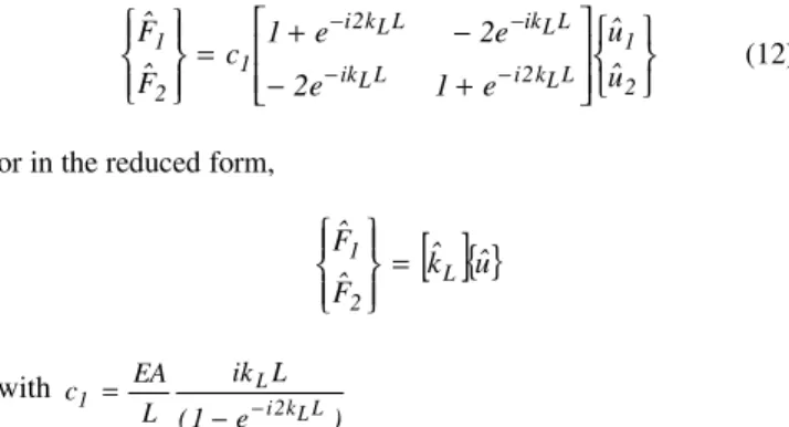
After the application of boundary conditions to a uniform wave-guide of finite length L with loads applied only to both ends, the system of equations for the bar element are given by,
+ − − + = − − − − 2 1 L L k 2 i L L ik L L ik L L k 2 i 1 2 1 uˆ uˆ e 1 e 2 e 2 e 1 c Fˆ Fˆ (12)
or in the reduced form,
[ ]
kˆ{ }
uˆ Fˆ Fˆ L 2 1 = with ) e 1 ( L ik L EA c L L k 2 i L 1 − − =where
k
ˆ
L is the dynamic stiffness matrix for the bar element, Fˆ is the complex amplitude vector of the applied force, uˆ is the vector of complex amplitudes of the node displacements andk
L is the wave number, defined as2 1 2 L EA A
k
= ω ρ (13)
In throw-off elements, waves propagate in one direction only. Thus, its dynamic stiffness matrix can easily be obtained by eliminating the term B in Eq. (11), which represents the reflected waves. Hence, the one-term dynamic stiffness for the single-node infinite element is given by,
L
iEAk
kˆ
L off throw L=
− (14)For the Timoshenko beam element, the four-coefficient exact solution is given by,
) x L ( 2 ik 2 ) x L ( 1 ik 1 x 2 ik 2 x 1 ik 1 ) x L ( 2 ik ) x L ( 1 ik x 2 ik x 1 ik e R e R e R e R ) , x ( vˆ e e e e ) , x ( ˆ − − − − − − − − − − − − − − + = + + + = D C B A D C B A ω ω φ (15)
where R1 and R2 are defined as the amplitude ratios and k1, k2 as the
wave numbers, all defined as,
+ − = + − = 2 2 2 2 2 2 2 2 1 2 1 1 I GA L EI GA iL R I GA L EI GA iL R ω ρ κ ξ κξ ω ρ κ ξ κξ 2 1 2 1 4 2 2 3 4 2 2 2 3 2 2 3 2 2 2 , 1 c c c 1 4 1 c c 1 c 1 2 1 ) ( k − + ± +
= ω ω ω
ω
(16) with the constants defined as
L k , L
k1 2 2
1 = ξ =
ξ 2 1 4 2 1 3 2 1 2 A I c , A EI c , A GA c ≡ ≡ ≡ ρ ρ ρ ρ κ
In the same manner as for the rod element, the throw-off beam element can be obtained by setting C=D=0.
These solutions can be written in terms of the nodal displacements, and a relation between the applied shear forces and moments and the nodal degrees of freedom can be established as,
{ }
[ ]
kˆ{ }
uˆ L EIFˆ B
3
= (17)
where
{ }
Fˆ =[
Vˆ1Mˆ1Vˆ2 Mˆ2]
T is the force vector and kˆB is the dynamic stiffness matrix. It is symmetric and complex for damped systems. The individual elements of this matrix can be found in Doyle (1997). An internal loss factor η can be included in all these wave numbers, to account for damping, by using a complex Young modulus E(1+iη). Only one element is needed between any two discontinuities, independent of its length. This plays the role of making the number of these elements in a 3-D structure relatively small. Thus, the response at different nodal degrees of freedom can be recovered with less computational cost by solving this system of equations at each frequency. These responses are then used to predict the total energy of a given structural element, for a certain wave type (longitudinal or flexural).SEM Model of the L-beam
The L-beam consists of two semi-infinite beams, beam 1 and beam 2, connected at a right angle. The SEM model uses two 2-noded and two throw-off spectral elements, as shown in Fig. 1. The throw-off elements are used in order to have no reflections at the free ends of the structure. The two beams have the following properties: A=0.01x0.01m2, E=2.62x10⁹N/m2, ρ=1280Kg/m3 and
L=100m for each of the 2-node elements.
beam 1
beam 2
P2in
P4in P1in
P3in
(2) (3) (1)
1 2 3
4 5 (4) (a) (b) x y throw-off element 2-noded element
Figure 1. (a) SEM model for the right angle beam; (b) power input in different subsystems.
Four subsystems are considered in this model: two for the longitudinal waves and another two for the flexural waves in the x-y plane. The power is input into one subsystem independently, say
1 in
ηB1B2 : CLF between flexural waves incident at beam 1 and
flexural waves transmitted to beam 2.
ηB1L2 : CLF between flexural waves incident at beam 1 and
longitudinal waves transmitted to beam 2.
ηL1B2 : CLF between longitudinal waves incident at beam 1 and
flexural waves transmitted to beam 2.
ηL1L2 : CLF between longitudinal waves incident at beam 1 and
longitudinal waves transmitted to beam 2.
(a)
(b)
(c)
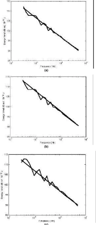
Figure 2. Coupling loss factors for the T-beam structure.
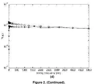
* CLF obtained via SEM using the simplified expressions of Stimpson & Lalor, ----o---- CLF obtained analytically via Cremer’s expressions.
(d)
Figure 2. (Continued).
A good agreement can be observed between the CLFs obtained by the proposed methodology and the CLFs obtained analytically. It is also observed that the estimations improve with frequency. It should be noted that, differently from what would happen when modeling with FEA, the SEM model will not deteriorate as frequency increases (provided the theory used still holds). It should also be noted that if the PIM had been used directly to compute the CLFs the results would be poorer when compared to those obtained using Eq. (7) due to the ill-conditioning of the linear system of equations of PIM method.
The CLFs obtained via the proposed methodology are then used in the SEA modeling of a T-shaped beam structure. This T-beam was used in a Round-Robin survey. It was constructed at the Naval Surface Warfare Center in Bethesda, Maryland, under the supervision of Dr. R. P. Szwerc. A complete description of the structure is given by Cuschieri et al. (1996) and is shown in Fig. 3 for clearance. The energy levels in the three beams of the structure calculated via SEA are shown in the following figures. Energy levels are calculated using the CLFs obtained via the proposed methodology and compared to those calculated via the analytical expressions given by Cremer et al. (1988). A frequency range from 1Hz to 5kHz is analyzed using a 1/3-octave scale with 50 frequency lines per band.
x y
z
A B
C
Material: Lexan E=2.62x10⁹ N/m2
ν=0.25 η=0.01
A=0.0317x0.054 m2
I=1.43x10⁻⁷ m4
LA=0.779 m LB=1.0827 m LC=0.9303 m
(a)
(b)
(c)
Figure 4. Energy levels in the T-beam; (a) Leg-A, (b) Leg-B, (c) Leg-C:
calculated with CLFs obtained using SEM/S&L, --- calculated with analytical CLFs.
It can be observed that the energy levels in the three legs of the T-beam predicted with SEA using the CLFs obtained via SEM/S&L compare very well with those obtained using analytical CLFs. It should also be noted that the differences decrease with frequency, as expected when using SEA.
Conclusions
Good SEA models require a reliable estimation of the coupling loss factors (CLFs). A methodology for computing CLFs based on the Spectral Elements Method (SEM) is proposed in this paper. Provided the underlying structural theory holds, the SEM has no high frequency limitations, as it utilizes exact interpolation functions. Analytical expressions for the CLFs can be found in the literature for beam structures connected at a right angle. Thus, the proposed methodology is applied to a right-angle beam and compared to the analytically obtained factors. The CLFs obtained numerically compare very well with the analytically obtained ones. Frame elements, which consist of a combined rod, shaft and beam element, can be used to obtain CLFs for different wave types propagating in 3-D frame-type structures. This allows the application of the proposed SEM-based methodology to frame-type beams joined at any arbitrary angles. The use of other types of spectral elements (such as plate elements) would permit obtaining the CLFs for other types of strucutral coupling such as plate-plate and plate-beam coupling. This will be feasible when more general, two-dimensional SEM elements become available.
Acknowledgements
The authors would like to thank FAPESP (Fundação de Amparo à Pesquisa do Estado de São Paulo) and CNPq (Conselho Nacional de Desenvolvimento Científico e Tecnológico) for the financial support.
References
Lee, U., Kim, J., and Leung, A. Y. T., 1999. “The Spectral Element Method in Structural Dynamics”. The Shock and Vibration Digest, 32(6), 451-465.
Lyon, R. H. and DeJong, R. G., 1995. “Theory and Applications of Statistical Energy Analysis”. Butter-worth-Heinemann, 2nd edition.
Maxit, L. and Guyader, J. L., 2001(a). “Estimation of Coupling Loss Factors Using a Dual Formulation and FEM Modal Information, part I: Theory”. Journal of Sound and Vibration 239 (5), 907-930.
Maxit, L. and Guyader, J. L., 2001(b). “Estimation of Coupling Loss Factors Using a Dual Formulation and FEM Modal Information, part II: Numerical Applications”. Journal of Sound and Vibration 239 (5), 931-948.
Ahmida, K. M., and Arruda, J. R. F., 1999. “Spectral Element Modeling of the Power Flow in a T-beam Structure: a Computational Experiment”, ASME Paper DETC99/VIB-8113, Proceedings of the 17th Biennial Conference on Mechanical Vibration and Noise, ASME Design Engineering Technical Conference, Las Vegas, September 12-15, CR-ROM, 7pp.
Ahmida, K. M. and Arruda, J. R. F., 2001. “Spectral Element-Based Prediction of Active Power Flow in Timoshenko Beams”, International, Journal of Solids and Structures, V38, No. 10-13, pp. 1669-1679.
Cremer, L., Heckl, M., Ungar, E. E., 1988. Structure-Borne Sound. Springer Verlag, 2nd edition.
Stimpson, G. and Lalor, N., 1991. Practical Noise Modelling of a Car Body Structures Using Energy Flow Analysis. Proc. Internoise, pp. 1233-1236.
Doyle, J. F., 1997. Wave Propagation in Structures. Springer-Verlag, New York, NY.
Cuschieri, J. M., Castagnet, E., E., LeFevre, T. A., Wilcox, T. E., 1996. SEA Modeling of the T-Beam. Proc. Noise-Con96, Bellevue, pp. 467-472.