Empirical evaluation of random wired neural networks

F

ACULDADE DE

E

NGENHARIA DA

U

NIVERSIDADE DO

P

ORTO

Empirical Evaluation of Random Wired

Neural Networks

João Mendes

Mestrado Integrado em Engenharia Informática e Computação Supervisor: Luís Teixeira

Co-Supervisor: Cláudio Sá Co-Supervisor: Žiga Emeršiˇc

Empirical Evaluation of Random Wired Neural Networks

João Mendes

Mestrado Integrado em Engenharia Informática e Computação

Approved in oral examination by the committee:

Chair: Prof. J. Magalhães Cruz

External Examiner: Prof. Peter Peer (University of Ljubljana) Supervisor: Prof. Luís Teixeira

Supervisor: Prof. Cláudio Sá

Supervisor: Prof. Žiga Emeršiˇc (University of Ljubljana)

Abstract

Artificial Neural Networks (ANN) are powerful and flexible models that perform learning tasks by considering examples, with a human-designed structure. However, architecture engineering of neural network models is one of the most time-consuming tasks. It involves trial and error which does not identify why a solution works and there are many hyperparameters to be adjusted.

Established networks like ResNet and DenseNet are in large part effective due to how they are wired, a crucial aspect for building machine learning models. For this reason, there have been some attempts to automate both the design and the wiring process. In this work, we study ap-proaches for network generators, algorithms that bypass the human intervention in neural network design.

From this starting point, we are looking for alternative architectures which in practice would be more difficult to design by humans using randomly wired neural networks. We conduct an empirical study to evaluate and compare the results of different architectures. With our findings, while analyzing the network behavior during training, we hope to contribute to future work on this type of neural network.

Our implementation of randomly wired neural networks achieves state of the art results, con-firming their potential. Our empirical study involves a grid search for the best parameters in the random graph models that are the foundation of these networks. The graph models generate ran-dom graphs that define the wiring of the network in three of its stages. We also perform a search for the best number of nodes present in the mentioned graphs. We find that a low number of nodes is enough to achieve similar performance to the state of the art results in our datasets. The range of parameters for the graph models is more extensive compared to the original study. The orig-inal results are replicable but not reproducible in the sense that if the origorig-inal experiments were conducted in the same conditions, we suspect that the stochastic nature of the network generator would yield distinct results.

Our optimization approaches lead us to conclude that the wiring of a network is important to allow more operations but the weights in the connections are nearly irrelevant. Avoiding using these weights, by freezing them, saves some training time while still reaching a good performance. The final thoughts of this work conclude that the network generator is one to be explored under the right resources and can contribute to the improvement of the field of NAS.

Keywords: Machine learning, Neural networks, Randomized search

Resumo

As Artificial Neural Networks (ANN) são modelos poderosos e flexíveis que executam tarefas de aprendizagem considerando exemplos, com uma estrutura definida por humanos. No entanto,

ar-chitecture engineeringde modelos de redes neuronais é uma das tarefas mais complexas. Envolve

tentativa e erro, o que não permite identificar porque uma solução funciona e contém diversos hiperparâmetros sujeitos a ajuste.

Redes já estabelecidas como ResNet e DenseNet são em grande parte eficazes devido à forma como são conectadas, um aspecto crucial para a construção de modelos de machine learning. Por esse motivo, houve algumas tentativas para automatizar o design e o processo de ligação. Neste trabalho, estudamos abordagens para geradores de redes, algoritmos que ignoram a intervenção humana no design de redes neuronais.

Deste ponto de partida, procuramos arquiteturas alternativas que, na prática, seriam mais difí-ceis de obter por seres humanos, usando redes neuronais ligadas aleatoriamente. Realizamos um estudo empírico para avaliar e comparar os resultados de diferentes arquiteturas. Com as nossas descobertas, ao analisar o comportamento da rede durante o treino, esperamos contribuir para o trabalho futuro neste tipo de rede neuronal.

A nossa implementação de redes neuronais randomly wired alcança resultados dentro do es-tado da arte, confirmando o seu potencial. O nosso estudo empírico envolve uma grid search pelos melhores parâmetros nos modelos de grafos aleatórios que são a base dessas redes. Os algoritmos para modelar grafos geram grafos aleatórios que definem as ligações da rede em três dos seus está-gios. Também realizamos uma busca pelo melhor número de nós presentes nos grafos menciona-dos. Concluímos que um número baixo de nós é suficiente para obter desempenho semelhante aos resultados de última geração nos nossos conjuntos de dados. A gama de parâmetros para os modelos de grafos aleatórios é mais extensa em comparação com o estudo original. Os resultados originais são replicáveis, mas não reproduzíveis, no sentido de que, se as experiências originais fossem conduzidas nas mesmas condições, suspeitamos que a natureza estocástica do gerador de

redesproduziria resultados distintos.

As nossas abordagens de otimização levam-nos a concluir que o wiring de uma rede é impor-tante para permitir mais operações, mas os pesos nessas conexões são quase irrelevantes. Evitar o uso desses pesos, ao congelá-los, economiza algum de tempo de treino e, ao mesmo tempo, atinge um bom desempenho.

As considerações finais deste trabalho concluem que o gerador de redes deve ser explorado com os recursos certos e pode contribuir para melhorias no campo de Neural Architecture Search.

Acknowledgements

Thank you to the University of Ljubljana, especially the Faculty of Computer Science for hosting me for a full academic year, providing resources that made this work possible.

For my parents, for all the support.

For my sister, for all the (maybe constructive) criticism. For my graduating friends back home, for all the memories. For my Erasmus friends, for all the adventures.

For my supervisors, for all the patience. To Edgar and Marie, in the back of the SAAB. Thank you all.

Aos Finalistas!

João Mendes

“Find what you love and let it kill you.”

Charles Bukowski

Contents

Resumo iii

1 Introduction 1

1.1 Context and Motivation . . . 2

1.2 Objectives . . . 3

1.3 Document Structure . . . 3

2 State of the Art 5 2.1 Introduction . . . 5

2.2 Neural Networks . . . 6

2.2.1 What they are . . . 7

2.2.2 How they work . . . 10

2.2.3 Computer Vision . . . 11

2.3 Randomly Wired Neural Networks . . . 12

2.3.1 Automatic generation of networks . . . 13

2.3.2 Random Graph Models . . . 14

2.3.3 Node Transformations . . . 16 2.3.4 Evaluation . . . 17 2.3.5 Structure Priors . . . 17 2.3.6 Process automatization . . . 18 2.4 Established Algorithms . . . 19 2.4.1 NAS . . . 19 2.4.2 NAS state-of-the-art . . . 20

2.4.3 Other Definitions in Machine Learning . . . 21

3 Methodology 23 3.1 Developing Environment . . . 23 3.2 Requirements . . . 24 3.3 Implementation . . . 24 3.4 Metrics . . . 26 3.5 Datasets . . . 26

3.6 Empirical Evaluation Experiments . . . 27

3.6.1 Network generator evaluation . . . 27

3.6.2 Node number evaluation . . . 28

3.7 Optimization Approaches . . . 28

3.7.1 Prediction of connection weights . . . 29

3.7.2 Freezingweights . . . 30

3.7.3 Weight shuffling . . . 31

x CONTENTS

3.7.4 Weight distribution . . . 31

3.7.5 Node shuffling . . . 31

4 Results and Evaluation 33 4.1 Problem State of the Art . . . 33

4.2 Empirical Study . . . 33

4.2.1 Network GeneratorHyperparameter Tuning . . . 34

4.2.2 Random Search . . . 38

4.2.3 Node Grid Search . . . 39

4.3 Optimization results . . . 41

4.3.1 Weight prediction . . . 41

4.3.2 Weight variation . . . 44

4.3.3 Weight sharing . . . 48

4.3.4 Main results . . . 49

5 Conclusions and Future Work 51 5.1 Conclusions . . . 51

5.2 Contributions . . . 52

5.3 Future Work . . . 52

A Appendix 1 55 A.1 Empirical Study . . . 55

A.2 Optimization Approaches . . . 55

A.2.1 Weight Variation . . . 55

A.2.2 Weight Sharing . . . 55

B Appendix 1 59 B.1 Graph Metrics . . . 59

C Appendix 3 61 C.1 Dataset Samples . . . 61

List of Figures

1.1 Comparison between building blocks of ResNet and DenseNet. . . 2

2.1 sigmoid function that is widely used in classification problems. It outputs val-ues between 0 and 1 and is nonlinear, so we can combine it with other sigmoid functions and stack layers. . . 8

2.2 8 nodes that represent layers . . . 14

2.3 The impact of probability p on the WS model [81]. . . 14

2.4 WS random graph model generated undirected graph. . . 15

2.5 DAG mapping from a NAS cell [91] . . . 16

2.6 Node operations for random graphs [86]. Input edges produce an (additive) ag-gregation, conv performs a Conv-ReLU-BatchNorm transformation block and the output edges represent the data flow distribution. . . 17

2.7 WS generated regular complexity regime networks [86] . . . 18

3.1 Focus on a single node connection, between nodes A and B through weight w1 . . 29

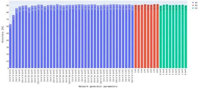
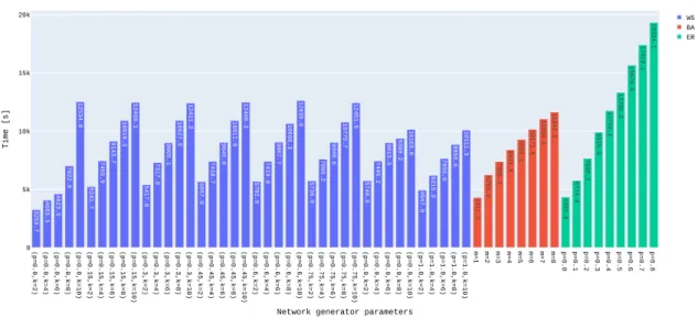
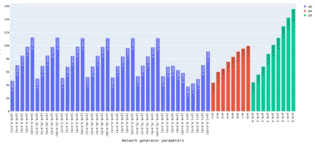
4.1 network generator’s θ parameters variation impact on CIFAR10’s accuracy . . . 34

4.2 network generator’s θ parameters variation reflected on CIFAR10’s training time. 35 4.3 θ network generator’s parameters variation impact on MNIST’s accuracy. . . 35

4.4 θ network generator’s parameters variation impact on MNIST’s training time. . . 36

4.5 θ network generator’s parameters variation impact on Fashion-MNIST’s accuracy. 36 4.6 θ network generator’s parameters variation impact on Fashion-MNIST’s training time . . . 37

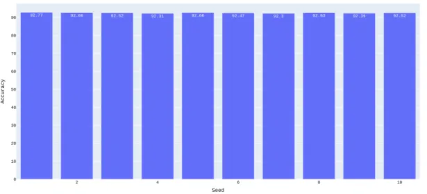
4.7 θ network generator’s parameters variation impact on CIFAR100’s training time 37 4.8 Seed variation impact on CIFAR10’s accuracy. These are the first generation net-works used on the optimization approaches in Section3.7 . . . 38

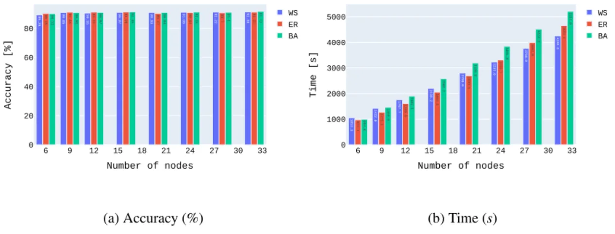
4.9 CIFAR10’s node count C study: accuracy (left) and time (right) . . . 39

4.10 MNIST’s node count C study: accuracy (left) and time (right) . . . 40

4.11 Fashion-MNIST’s node count C study: accuracy (left) and time (right) . . . 40

4.12 CIFAR100’s node count C study: accuracy (left) and time (right) . . . 41

4.13 Considering features with an importance larger than 0.005 . . . 42

4.14 Optimizer influence on accuracy on the CIFAR10 [42] dataset . . . 43

4.15 Evaluation for shuffling a connection weight prediction for 100 iterations in CI-FAR10. The standard deviation in the shuffled bar is 0.25. . . 44

4.16 Example of weight distribution in a network, with standard deviation of 0.283 and mean of 0.109 . . . 45

4.17 Accuracy evolution of several approaches on the CIFAR10 [42] dataset . . . 45

4.18 Training time of several approaches on the CIFAR10 [42] dataset . . . 46

xii LIST OF FIGURES

4.19 Training accuracy evolution of several approaches on the Fashion-MNIST [84]

dataset . . . 47

4.20 Training time of several approaches on the Fashion-MNIST [84] dataset . . . 48

4.21 Training evolution of shared weights on the Fashion-MNIST [84] dataset . . . . 49

A.1 θ network generator’s parameters variation impact on CIFAR100’s accuracy . . . 55

A.2 Training accuracy evolution of several approaches on the MNIST [46] dataset . . 56

A.3 Training accuracy evolution of several approaches on the CIFAR10 [42] dataset . 56 A.4 Training accuracy evolution of several approaches on the CIFAR100 [43] dataset 56 A.5 Evaluation for shuffling a connection weight prediction for 100 iterations in CI-FAR100 . . . 57

A.6 Untrained valuation for shuffling a connection weight prediction for 100 iterations in CIFAR100 . . . 57

A.7 Training evolution of shared weights on the MNIST [46] dataset . . . 57

A.8 Training evolution of shared weights on the CIFAR10 [42] dataset . . . 58

A.9 Training evolution of shared weights on the CIFAR100 [43] dataset . . . 58

C.1 CIFAR10’s [42] image samples . . . 61

C.2 CIFAR100’s [43] image samples . . . 62

C.3 MNIST’s [46] image samples . . . 62

List of Tables

3.1 The general network architecture, as seen in the small regime [86]. . . 27

3.2 Default θ parameters used in the original study [86] . . . 28

4.1 Dataset SotA survey . . . 33

4.2 Performance of several attempted optimization approaches . . . 48

B.1 This table describes the features used in the machine learning algorithm. The features marked with “x” in the NetworkX column were directly obtained from the NetworkX library [26]. The remaining features were calculated. . . 60

Abbreviations

DL Deep Learning

ML Machine Learning

NN Neural Network

NAS Neural Architecture Search

ANN Artificial Neural Networks

RNN Recurrent Neural Network

CNN Convolutional Neural Network

DNN Deep Neural Network

WS Watts-Strogatz random graph model

ER Erd˝os and Rényi random graph model

BA Barabási-Albert random graph model

CPU Central Processing Unit

GPU Graphic Processing Unit

AutoML Automated Machine Learning

AI Artificial Intelligence

MLP Multi-layer Perceptrons

SGD Stochastic Gradient Descent algorithm

LSTM Long Short-Term Memory

GRU Gated Recurrent Unit

TCN Temporal Convolutional Networks

ReLU Rectified Linear Unit

RL Reinforcement Learning

DAG Directed Acyclic Graph

FLOPs FLoating point OPerations

Chapter 1

Introduction

Machine Learning evolved from pattern recognition and the idea that computers could learn

with-out explicit programming [76]. Like with humans, or computers with machine learning, learning

comes from experience in a certain task. This experience stems from analyzing large amounts of data and the quality of the data is important for the success of the machine learning model. Math-ematical models are built by machine learning algorithms from training data. The model should be able to generalize from experience and make successful predictions on new examples. Several types of algorithms have been developed for machine learning and one of the most popular are Artificial Neural Networks.

Artificial Neural Networks are inspired by biological neural networks [68], having simple

interconnected processing nodes. Nodes are usually organized into layers that are responsible for operating at a specific depth. The input layer receives data and the output layer produces an output given the information passed through the network. The hidden layers is usually where most of the learning happens and our knowledge of the behavior is weaker. Each node has a set of weights and biases for their inputs and computes an output using an activation function.

Deep learning, also known as deep neural learning, is too a subset of machine learning

algo-rithms that uses a connectionist approach to develop networks [86]. Higher-level features are

pro-gressively extracted from a dataset using multiple layers. The neural network phenomena success has led to a focus transfer from feature engineering to a more abstract level, architecture engi-neering. In other words, although feature engineering has become simpler through deep learning, machine learning models architecture has become consequently more complex. Some problems may require such a specific architecture that it becomes a task similar to past feature engineering obstacles.

Current methods still significantly involve human effort and are short of achieving AutoML. The goal is not to automatize ML but to show the potential in AutoML by bringing us a step closer in its direction. Researchers are trying to automate the process of applying machine learning to real-world problems, aiming for simpler solutions and faster creation of models. Neural networks

2 Introduction

are built using building blocks that are usually small and manually designed, plus a set of con-straints is applied to their architecture. We are a long way from having self-designed, adaptable networks that cover the complete pipeline. Google provides a service, “Cloud AutoML” that aims

to fulfill these needs [29] [74], from the initial dataset to a fully working machine learning model.

A lot of work is being done towards that goal and we hope that this research contributes to the field.

From the equation 4 and equation 6, we can see that

the standard convolution layer required 9 × chout

operations

where as depth-wise separable 3 × 3 convolution layer

followed by 1 × 1 convolutions required only 9 + ch

out

oper-ations. In this study, we used MobileNet-v1 with 0.5x and 1x

channels multiplier with input size of 224 × 224 for testing.

These models are denoted as M obileN et V 1 0.5 224 and

M obileN et V 1 1.0 224, respectively, in Table I.

5. MobileNet-V2: The newer version of MobileNet

ar-chitecture combines depth-wise separable 3 × 3 convolution

with inverted ResNet architecture. In ResNet architecture, as

shown in Figure 1(a), the 3 × 3 convolution is performed

on the reduced number of channels whereas in

MobileNet-v2 [16] architecture the 3 × 3 convolution layer is replaced

with depth-wise separable 3 × 3 convolution layer and

increased number of channels, as shown in Figure 1(b). if

ch

in

are the number of feature channels provided as an input

to the residual layer, resnet architecture extracts features at

3 × 3 convolution on half of the input feature channels i.e.,

ch

in/2. Whereas in the case of MobileNet-V2, the feature

channels are increased by an expansion factor t i.e., chin

∗ t.

In our experiments, we used MobileNet-v2 with 0.5x and

1x channels multiplier with input size of 224 × 224 for

testing. These models are denoted as MobileNet V2 0.5 224

and MobileNet V2 1.0 224, respectively, in Table I.

6. NasNet-Mobile: Unlike other models presented in this

paper, this model has not been designed by hand. Instead,

a reinforcement learning technique known as AutoML[20]

was used to generate this model, and specifically designed

to perform well over Imagenet[19] dataset. AutoML searches

for the best convolutional layer (or cell) on a small dataset

and then transfer the block to a larger dataset. By changing

the number of the convolutional cells and number of filters

in the convolutional cells, different versions of NASNet[18]

were developed. In this paper, we considered the smallest

of all the NasNets, called NASNet-mobile, which is targeted

for mobile devices.

7. Proposed Model: Our custom model is based on

MobileNet-v2 architecture, as shown in Figure 1(d), where

we keep expansion factor t = 1. Table II show the complete

architecture of the proposed model. As it can be seen from

the Table II, the spatial resolution is dropped 4X

with-in first two layers to reduce the computational complexity.

The convolution layers conv2, conv3 and conv4 use the

residual module shown in Figure 1(d). At conv2b and conv3b

same module is used but without the skip connection to

reduce spatial resolution by half and to increase the number

of feature channels. The proposed model has only 672K

parameters and 256M MAdd operations. The feature size

and number of parameters in our proposed model are the

least among all the models (see Table I).

III. E

XPERIMENTAL

V

ALIDATION

: A C

ASE

S

TUDY ON

O

CULAR

B

IOMETRICS

Dataset: VISOB [21] dataset consists of ocular

im-ages [22] from over 550 healthy subjects. This publicly

available dataset was collected using front-facing cameras

Fig. 1. (a) Resnet architecture (b) MobileNet-V2 architecture (c) DenseNet architecture (d) Custom layer module similar to MobileNet-V2 architecture with expansion factor t = 1 and with normalization and activation before each convolutional layer.

of different mobile devices (iPhone 5s, Samsung Note 4

and Oppo N1) under varying lighting conditions (office,

daylight and dim indors). Participants’ data were collected

in two visits, visit 1 and visit 2, 2 to 4 weeks apart. During

each visit, participants took a selfie like captures in two

different sessions (session 1 and session 2) that were about

10 to 15 minutes apart, under all lighting conditions and

using all the three devices. From the collected data, eye

crops were generated using Viola-Jones based eye detector

and the cropped eye images were resized to 160 × 240

pixel resolution. Variations such as motion blur, specular

reflections, and different lighting conditions are captured in

this dataset. Figure 2 shows example ocular images from

VISOB dataset.

In our experiments, we divided VISOB dataset into three

sets as follows:

1) DATA-A: This set consists of ocular images from

200 participants from Visit 1 for all the devices, all

(a) ResNet [28] architecture [17]

From the equation 4 and equation 6, we can see that

the standard convolution layer required 9 × chout

operations

where as depth-wise separable 3 × 3 convolution layer

followed by 1 × 1 convolutions required only 9 + chout

oper-ations. In this study, we used MobileNet-v1 with 0.5x and 1x

channels multiplier with input size of 224 × 224 for testing.

These models are denoted as M obileN et V 1 0.5 224 and

M obileN et V 1 1.0 224, respectively, in Table I.

5. MobileNet-V2: The newer version of MobileNet

ar-chitecture combines depth-wise separable 3 × 3 convolution

with inverted ResNet architecture. In ResNet architecture, as

shown in Figure 1(a), the 3 × 3 convolution is performed

on the reduced number of channels whereas in

MobileNet-v2 [16] architecture the 3 × 3 convolution layer is replaced

with depth-wise separable 3 × 3 convolution layer and

increased number of channels, as shown in Figure 1(b). if

ch

in

are the number of feature channels provided as an input

to the residual layer, resnet architecture extracts features at

3 × 3 convolution on half of the input feature channels i.e.,

ch

in/2. Whereas in the case of MobileNet-V2, the feature

channels are increased by an expansion factor t i.e., chin

∗ t.

In our experiments, we used MobileNet-v2 with 0.5x and

1x channels multiplier with input size of 224 × 224 for

testing. These models are denoted as MobileNet V2 0.5 224

and MobileNet V2 1.0 224, respectively, in Table I.

6. NasNet-Mobile: Unlike other models presented in this

paper, this model has not been designed by hand. Instead,

a reinforcement learning technique known as AutoML[20]

was used to generate this model, and specifically designed

to perform well over Imagenet[19] dataset. AutoML searches

for the best convolutional layer (or cell) on a small dataset

and then transfer the block to a larger dataset. By changing

the number of the convolutional cells and number of filters

in the convolutional cells, different versions of NASNet[18]

were developed. In this paper, we considered the smallest

of all the NasNets, called NASNet-mobile, which is targeted

for mobile devices.

7. Proposed Model: Our custom model is based on

MobileNet-v2 architecture, as shown in Figure 1(d), where

we keep expansion factor t = 1. Table II show the complete

architecture of the proposed model. As it can be seen from

the Table II, the spatial resolution is dropped 4X

with-in first two layers to reduce the computational complexity.

The convolution layers conv2, conv3 and conv4 use the

residual module shown in Figure 1(d). At conv2b and conv3b

same module is used but without the skip connection to

reduce spatial resolution by half and to increase the number

of feature channels. The proposed model has only 672K

parameters and 256M MAdd operations. The feature size

and number of parameters in our proposed model are the

least among all the models (see Table I).

III. E

XPERIMENTAL

V

ALIDATION

: A C

ASE

S

TUDY ON

O

CULAR

B

IOMETRICS

Dataset: VISOB [21] dataset consists of ocular

im-ages [22] from over 550 healthy subjects. This publicly

available dataset was collected using front-facing cameras

Fig. 1. (a) Resnet architecture (b) MobileNet-V2 architecture (c) DenseNet architecture (d) Custom layer module similar to MobileNet-V2 architecture with expansion factor t = 1 and with normalization and activation before each convolutional layer.

of different mobile devices (iPhone 5s, Samsung Note 4

and Oppo N1) under varying lighting conditions (office,

daylight and dim indors). Participants’ data were collected

in two visits, visit 1 and visit 2, 2 to 4 weeks apart. During

each visit, participants took a selfie like captures in two

different sessions (session 1 and session 2) that were about

10 to 15 minutes apart, under all lighting conditions and

using all the three devices. From the collected data, eye

crops were generated using Viola-Jones based eye detector

and the cropped eye images were resized to 160 × 240

pixel resolution. Variations such as motion blur, specular

reflections, and different lighting conditions are captured in

this dataset. Figure 2 shows example ocular images from

VISOB dataset.

In our experiments, we divided VISOB dataset into three

sets as follows:

1) DATA-A: This set consists of ocular images from

200 participants from Visit 1 for all the devices, all

(b) DenseNet [34] architecture [17]

Figure 1.1: Comparison between building blocks of ResNet and DenseNet.

Established networks, like ResNet [28] and also DenseNet [34] – compared in Figure1.1,

per-form well because of their innovative connections. ResNet introduced skip connections to prevent the degradation of the accuracy in deeper layers of the network. The method stacks additional layers as residual blocks which are identity mappings, implying no extra parameters to train. This process benefits the deeper layers to perform more similarly to the shallower ones. In DenseNet, layers are connected to all their preceding layers. The final classifier will then have information from all feature-maps because the information was preserved through these extra connections. Thus, how the computational networks are wired is crucial for their performance. Just like the human brain, where wiring and connectivity are important not only to prevent malfunction but to

achieve peak performance [30], we can have an immeasurable amount of wiring combinations.

1.1

Context and Motivation

Neural Architecture Search is a technique for automating the design of neural networks. One of the

first proposed algorithms [90], has a set of building blocks as a starting point and uses an Artificial

1.2 Objectives 3

the problem at hand. The network is subject to training and testing, and, based on the results, the blocks can be adjusted to obtain a better performing network.

The search space of NAS algorithms is too extensive to be explored manually [83], even though

researchers have discovered some successful designs. The idea is to evaluate the potential of randomly wired neural networks to traverse the search space without human intervention to design the architectures. One of the motivations is that researchers have found that state-of-the-art NAS

algorithms perform similarly to a random architecture selection [69] where it would be expected

that an effective search policy significantly outperforms a random one.

The authors in [86] proposed future work in this area to explore new network generator designs

that may yield new, powerful network designs. These network generators are inspired in classical

random graph models [5] from random graph theory, used to reduced bias. They are based in

different probabilistic distributions which could have predictable outcomes to some degree. The use of other tools to generate random graphs is an option to do comparisons with the currently used models.

This work extends the previous work in [86] through empirically testing their proposed

ap-proach and derive conclusions that could lead to the expansion of the NAS search space.

1.2

Objectives

The goal is to implement network generators by means of a random policy and use them to generate several architectures. Collecting these architectures, we evaluate the performance, compare the results with state-of-the-art solutions, and draw conclusions. From this empirical study, we attempt to gather useful insights that might support new solutions for the NAS. We use machine learning algorithms to predict part of the initial weights of the randomly wired networks before training to boost training in duration or an earlier convergence.

1.3

Document Structure

Firstly, the document exposes the literature related to this study in Chapter2, where we go through

definitions and related work. In Chapter3, we describe our methods and different approaches to

study randomly wired neural networks. In Chapter4we present our results with graphical aid and

justify our thought process in the iterative experimental procedure. Finally, in Chapter5we submit

Chapter 2

State of the Art

In this chapter, we start by giving a short introduction to how the field of Machine Learning evolved through the years. Then we present some concepts to contextualize neural networks and how they

came to be. We focus on Randomly Wired Neural Networks in Section2.3, providing an in-depth

description of how they are built. Furthermore, we review the state of the art of Neural Network algorithms.

Neural architecture search (NAS) is, arguably, the next big challenge in the field of deep

learning [76]. With NAS, one can use a model to look for better architectures given a specific

type of data, rather than being limited to trial and error search. NAS algorithms can become even more powerful when we look for alternative architectures which in practice would be more difficult to design by humans. This has the potential for discovering truly novel architectures. In this section, we present these concepts and the state-of-the-art of the field.

2.1

Introduction

Machine Learning (ML) has contributed to the success in the ongoing digital change across in-dustries, like transportation, healthcare, finance, agriculture, and retail. This favorable outcome is

long overdue because machine learning is not new [52] since machine learning exists for over 70

years [40]. The explosion of computing power and hardware enhancement has allowed pursuing

ideas that have been around for decades but were not feasible before [3]. One of the ideas was to

make a machine learn: it performs a task by studying a set of examples – a training set. Then the same task is to be performed using unseen data. This comes hand in hand with the Artificial Intel-ligence (AI) definition where a machine can perceive its environment and takes action to achieve

its goals [63]. Other examples of important machine learning findings, involve activation functions

(Leaky ReLU [87]) and dropout, where some neurons are chosen at random to be ignored during

training.

6 State of the Art

Since the early days of AI that problems have become ever complex, causing smaller subsets of machine intelligence to appear. More recently, one of these subsets of ML emerged and is es-tablishing itself in the field for solving a multitude of computer science problems, known as Deep Learning (DL). It impacts areas including computer vision, speech recognition, robotics, network-ing, and gaming. DL is a branch of Machine Learning using algorithms that aim to represent

high-level data abstractions by constructing – complex – computational models [19]. Deep neural

networks are one of the most familiar deep learning structures, characterized by having multiple

levels of non-linear mathematical operations [6].

Similarly to ML, deep learning can be categorized in unsupervised, supervised, or partially

su-pervised approaches [3]. The first, unlike supervised learning, does not make use of labeled data

and relies purely on its internal representation to discover patterns within the input data. As the name suggests, partially unsupervised approaches rely on partially labeled data. Deep Reinforce-ment Learning is a more recent developReinforce-ment that successfully combines the ReinforceReinforce-ment

Learn-ing Paradigm of ML and artificial neural networks [57]. Supervised and Unsupervised Learning

includes the use of Convolutional Neural Networks (CNN), Deep Neural Networks (DNN), and Recurrent Neural Networks (RNN), which are the most common types. Reinforcement Learning uses goal-oriented algorithms, operating in a delayed return environment, and allows us to solve

complex decision-making tasks [20].

2.2

Neural Networks

Neural networks are a powerful and important technique in Machine Learning. In the early ’40s, using simple logic gate operations, it was proven that the combination of neurons can construct a

Turing machine [54]. In the late ’50s, Rosenblatt [65] shows that if the learning data can be

rep-resented, perceptrons will be able to converge. Here the neural networks appeared and since then they have been around for decades. This was the earliest neural network and it was used for binary classification. Because of this, there was a tremendous amount of investment and development in neural networks for decades.

There was a common belief that these neural networks are mimicking some of the functionality in biological systems and animals, like humans. Both the neuroscience and computer science communities had an interest in what were the capabilities of these networks. Limitations in the data (size and labeling) and the computational power at the time, caused a delay in research in the

late 70s and 80s in what is known as the "AI winter" [53]. Besides, in ’69, Minsky [55] exposes

the limitations of the neural network’s foundation, the perceptron, and the research is frozen for almost a decade.

There were several developments in the ’80s, the backpropagation algorithm was proposed

by Hinton et al [1] which re-energizes the field. A couple of years later, the Neocognitron [21]

hierarchical neural network emerges and is capable of recognizing visual patterns. In 1999, back-propagation is coupled with Convolutional Neural Networks and applied to image-based document

2.2 Neural Networks 7

analysis [45]. In 2006, the training problem for Deep Neural Networks is solved by the Hinton

Lab [31] using a greedy algorithm.

There was an overhyping of capabilities and the actual architectures could not deliver

be-cause of limitations of training time. These fell out of fashion until 2012, with the ImageNet [67]

challenge. Here, deep neural networks were trained on vast datasets in new computational archi-tectures, GPUs (graphics processing units). The challenge evaluates algorithms for image clas-sification and object detection at large scale, thus requiring complex solutions. This culmination of big data, big label datasets, and much more powerful computers that could facilitate the train-ing of deep neural network architectures was the revivtrain-ing point for neural networks. In 2012 the community was surprised by how significant the performance improvement in neural networks

had become. AlexNet [44] reduced the error rate by roughly half (from 26.2% to 15.3%) of the

previous state-of-the-art in this image classification challenge using Convolutional Neural Net-works. Since then, in a very short period, neural networks have risen to the top of the performance

metrics [28] [34] in many challenges both in speech recognition, natural language processing,

ma-chine translation, and image classification. Now they are setting the standard for what is possible in these and other applications where you have huge data sets and you want to do arbitrary function approximation or interpolation based on your training data set.

Neural networks are inspired in principle by biological systems [68]. Human motion and

deci-sion making are controlled by its brain, with a network of neurons that are performing incredibly complex tasks. There is a lot of research in neuroscience and computer science fields to see what kind of connections and comparisons we can make. What can we learn from biological systems that will help our neural networks? What can we learn when we build and design these neural

networks that can teach us about these biological systems? This is inspired by visual systems [21],

in particular this kind of multi-layered information processing architectures where you take very

high-resolution information and pass it through layers of abstraction [49]. Humans can easily

detect objects in motion and abstract what a certain collection of pixels represents, based on our previous experiences and abstractions. That is the kind of process we want our neural network to be able to do: take a complex input data and distill out through layers and processing different abstractions that we can use to build models.

2.2.1 What they are

Neural networks are at the lowest level consisted of neurons. These units take two or more inputs, perform mathematical operations using them – typically a weighted average – and produce one output. Each input is affected by its weight and the result of the sum is tuned with a bias. The final result is then used as an input to an activation function which normalizes it to a certain range. The

sigmoidfunction is commonly used:

which defines the output to be in the range [0, 1]. This process is known as feedforward, where

the data flows in only one direction. This basic unit is called perceptron [55], a mathematical

model of the biological neuron. A neural network is a group of connected perceptrons. There are an input and an output layer, and at least one hidden layer. Shallow neural networks have

8 State of the Art

−6 −4 −2 0 2 4 6

0.5 1

Figure 2.1: sigmoid function that is widely used in classification problems. It outputs values between 0 and 1 and is nonlinear, so we can combine it with other sigmoid functions and stack layers.

one hidden layer as opposed to Deep Neural Networks (DNN), which have several and often of different types. Multi-layer Perceptrons (MLPs) are a basic type of feedforward neural networks and are used for simple tasks. MLP can have several layers, whilst in DNN we assume there is a considerable number of layers and perceptrons.

Neural Networks use the gradient descent method to find an objective function’s local min-ima. Having a long training time has a drawback, we use optimizers to train these networks, for

example, the Stochastic Gradient Descent algorithm (SGD) [7]. Using backpropagation [66] the

neural network knows how every node is responsible for the total loss and takes action updating

weights accordingly [3]. The step size chosen during training is known as learning rate, it affects

how much the weights are updated.

The human visual processing system is more similar to Convolutional Neural Networks (CNNs) than DNNs. They are mostly used for image/video tasks and use filters and pooling to extract fea-tures from the raw data. They make use of the convolutional layer, where filters are applied to an image in several windows, the sliding through the image is known as convolution. The pooling layer – or down-sampling – is a layer in which the dimension of the feature maps is reduced, hav-ing less computational demand and parameters. The final layer is the output layer, wherein the case of classification, the score of each class is computed.

Some popular state-of-the-art CNN architectures include:

• AlexNet [44], a large, deep CNN introducing the dropping out of nodes to reduce overfitting;

• VGGNet [70] asserts the depth of a network as a critical aspect to achieve better performance

in CNNs;

• GoogLeNet [72] presented a less computational complex model with the concept of

2.2 Neural Networks 9

multiple pooling and filters layers simultaneously;

• DenseNet [34] was named because of the dense connectivity between layers. The outputs

of each layer are connected with all successor layers;

• ResNet [28] is a traditional feedforward network with emphasis on the depth that uses

resid-ual functions concerning the layer inputs for learning, these blocks allow the flow of infor-mation from initial layers to last layers;

• MobileNets [33] are lightweight deep neural networks, using hyperparameters to work on

different mobile phones while maximizing accuracy;

• EfficientNet [73] that creates a compound scaling hyperparameter affecting three

dimen-sions of a network: width, depth and resolution;

• Xception [11] uses depth-wise separable convolution layers, while being based on GoogLeNet

(also known as part of the Inception family of architectures);

• ResNeXt-50 [85] is related to ResNets and explores the concept of “cardinality” which

describes the repetition of a building block with the aggregation of transformations of the same topology.

Human thinking has implicit previous knowledge drawn from the past. Traditional neural networks are not prepared to handle historical information. Both their input and output are fixed-size vectors and have their computational steps also fixed (number of layers). In Recurrent Neural

Networks (RNNs), a loop passes the information from one step of the network to the next [37].

To compute an output, they use processed information from previous time steps. They are mostly used for sequential data, allowing input of any length. Plain RNNs suffer from the vanishing

gradient problem, where for very big sequences the gradient is too small to update the weights [60].

Different solutions have been proposed to solve this issue. The following examples are two of the most commonly used:

• Long Short-Term Memory (LSTM) [23] is based on a cell that remembers values over

dif-ferent time intervals, using three gates to regulate information flow (input, output, forget gates);

• Gated Recurrent Unit (GRU) [13] is similar to LSTM with fewer parameters and less

com-putationally expensive, using a simple update gate that combines the input and forget gates. These are layers that can be combined with convolutional layers. Video analysis and text processing are some of the applications.

More recently, Temporal Convolutional Networks [4] (TCNs) have achieved good

perfor-mances in sequence modeling tasks. TCNs take a sequence of a given length and produce an output of the same length whilst in RNNs it can also be larger or smaller. Even though they use

10 State of the Art

1D convolutions, these are causal, which implies that the information from the future to the past is not lost. These convolutions use elements from a moment in time m and earlier in the previ-ous layer to operate. Because the filters are shared across a layer, parallelism is possible, and the

required memory for training is reduced. More recently, the Transformers [79] were shown to be

superior in quality, more parallelizable because they can process unordered sequential data and require less time to train.

2.2.2 How they work

The learning part of the process is the training of the neural network. In this research, mostly su-pervised learning methods with fully labeled data will be used so we focus on processes involving those techniques. Firstly, the network is fed with training data, that traverses through the layers until its final prediction is calculated.

2.2.2.1 Layers

All the neurons, or at least part of them, affect their respective inputs from the previous layer and pass them to the next layer. At the end of this process, the final layer will output a prediction for the input example.

Batch normalization [36] is a technique that for each mini-batch standardizes the inputs to a

layer. The reasons for the effectiveness to improve stability, speed, and performance of ANN’s remain under discussion but the effect is evident.

2.2.2.2 Activation Functions

Activation functions define the output of a neuron. We have mentioned the sigmoid function2.1

but there are more:

• linear: identity function;

• tanh: hyperbolic tangent function, is a rescaling of the sigmoid function with range [-1,1]; • softmax: probability distribution of classes where the sum is 1 and the range is [0,1]; • ReLU(rectified linear unit): activates a node if the input is above a certain threshold. These functions are not very complex because they are computed at every neuron. Their derivatives can also be used. This means activation functions have an impact on the computational cost of the network.

2.2.2.3 Losses

A differentiable loss function is defined to estimate the error, to compare the prediction to the correct result. An error of – in a perfect world – zero, means that our predicted values do not

2.2 Neural Networks 11

diverge from the real values. This is never the case in Machine Learning, although the goal is to minimize this function. To improve the predictions, the weights of the neuron connections will be fine-tuned during training. Once this loss is calculated, its value is propagated backward, thus backpropagation.

The total signal of the loss is distributed according to the relative contribution of each neuron. The weights of connections between neurons are adjusted based on this information using the gra-dient descent technique. This helps detect which direction to shift the weight, using the derivative of the loss function. The process can be applied to batches of data that we feed the network in each iteration eventually passing through all the dataset – epoch.

2.2.2.4 Optimizers

To minimize the loss, we can use optimizers to adjust weights and biases. These parameters are not solvable analytically but can be approached using optimization algorithms such as the mentioned stochastic gradient descent where a few samples are randomly selected in each iteration to reduce computational costs.

Parameters are configurations internal to the model whose values are estimated from the data whilst hyperparameters are configuration variables external to the model and are specified by the user. This is where the creation of architectures in Deep Learning becomes complex, but human learning – or experience – is key. Some of these hyperparameters include activation functions, number of neurons, and number of layers at the topology level. At the learning algorithm level for example the number of epochs, the batch size, the momentum, and the learning rate.

The learning rate decay decreases the learning rate epoch by epoch, which allows earlier faster learning. It is progressively fine-tuned to ease the training convergence to a loss function min-imum. In real cases, this function is complex and the optimization process may be stalled on a local minimum, leading to sub-optimal results. Momentum addresses this problem by taking a weighted average – constant with range [0,1] determined by the user – of the previous steps to determine the direction of the gradient.

Although not exactly a hyperparameter, the initialization of parameter weights is important to reduce the number of epochs needed to train deep networks and stabilize the learning process.

2.2.3 Computer Vision

Computer Vision is a field of AI that makes use of computing systems to interpret the real world, by locating and identifying objects accurately through images and video. Deep Learning is widely

used in Computer Vision [71] with applications in important areas like Medicine, Autonomous

Vehicles, Military, and Machine Vision. Before deep learning, traditional computer vision meth-ods relied on hand-crafted features, which are not feasible for the current problems the field tries to tackle.

Some Computer Vision problems approached by Deep Learning [80]:

12 State of the Art

• Object Detection: detecting instances of objects inside images and/or video; • Image Retrieval: a collection of images having at least the one same object; • Semantic Segmentation: linking each pixel in an image with one class label; • Object Tracking: following a specific object in a scene;

• Action and Activity Recognition: sports and urban settings using input video sequences or images;

• Various Biometrics Tasks: from how to recognize subjects, to pose estimation and tracking, crowd counting, gaze estimation, etc.

These are some of the problems currently approached with deep learning. CNN’s are used in most of them because of feature learning as a unique capability although they rely heavily on

labeled data [71]. Being one of the most popular fields to deal with real-world problems [80],

computer vision is an optimal field to one who studies neural networks. Their extensive use in the

field and the wide variety of datasets (Section3.5) makes Computer Vision an interesting domain

to study.

2.3

Randomly Wired Neural Networks

Neural networks are inspired by the brain, although when we are young we lack the experience to learn and we rely on innate behaviors that are already present at birth. This suggests that animals

are born with highly structured brain connectivity, enabling them to learn rapidly [89], hence

biologists suggest the importance of wiring when building Artificial Neural Networks.

Searching the possible space of wirings – or connectivity – of neural networks can lead to more

efficient solutions [83]. In [83], the typical notion of layers is relaxed and, although the wiring

is fixed, as weights are modified during training, the higher k weights are dynamically selected. This threshold edge swap allows learning the connectivity as it learns the network parameters. The importance of wiring is also emphasized when using randomly initialized weights in network

architecture, performing no training, and still achieving success [22] in simple tasks.

Randomly wired hardware and its implementation in software (i.e. artificial neural networks) were an interest in the early stages of artificial intelligence. In the resurgence era of hardware, engineers were inspired by randomly wired hardware to apply them in software. Alan Turing

proposed unorganized machine [75], a concept comparable to a model of randomly connected

neural networks. In the 1950s, Rosenblatt [65] built a visual recognition machine based on an

array of photocells that was randomly connected and Minsky [56], implemented, using vacuum

tubes, one of the first learning neural network machines.

Random graphs are also generally studied in graph theory because they show different

2.3 Randomly Wired Neural Networks 13

G= (V, E, φ ) where V and E describe vertices (nodes) and edges (links), respectively. φ is a

func-tion that maps edges to an unordered pair of vertices. They are linked to natural phenomena and

are thus an effective means to model real-world problems like a computer or social networks [86].

The Facebook AI Research team recently presented a study [86] exploring the design of

network generators based on graph theory algorithms to generate random graphs. Searching for connectivity patterns at random is less design demanding than conducting a manual architecture construction.

Previously the main direction with ANN studies would rely on network engineering and learn millions of parameters (features, internal filters, and classifier weights) while this study uses net-work generator engineering to learn the netnet-works themselves.

2.3.1 Automatic generation of networks

A network generator is defined as g : Θ 7→N , where g is a mapping from a parameter space Θ

to a space of neural architecturesN . The parameters θ ∈ Θ define a network instance. E.g., in a

ResNet [28] generator some of the parameters could be the depth, width, number of stages, etc.

For g(θ ), mapping is deterministic, meaning we get a consistent output (network architecture N) when introducing the same input (parameters theta). To build a random family of networks, a seed s is introduced. It is obtained through a pseudo-random number generator and its value is changed while keeping the parameters θ fixed. g(θ , s) is referred to as a stochastic network generator.

In [91] this type of network generators were explored but contained several generation rules

applied to the network mapping coupled with the use of LSTM and other hyperparameters. The resulting network space is highly restricted by human design, involving a strong prior that reduces the subset of all possible graphs.

The (stochastic) network generator encapsulates different operations:

• Generating random graphs;

• Mapping graphs into a neural network; • Placing node and edge operations; • Introduce heuristic rules.

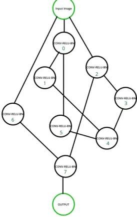
A random graph helps reduce human design in a neural network. Usually, CNN follows a

sequential pre-determined order when performing its operations. In Figure2.2, the different nodes

would follow this rule. The input, e.g. an image, is passed to the first node and follows an order accordingly. Randomly wired neural networks have a different approach, where the network’s flow is arbitrarily defined while still being sequential.

14 State of the Art CONV-RELU-BN CONV-RELU-BN CONV-RELU-BN CONV-RELU-BN CONV-RELU-BN CONV-RELU-BN CONV-RELU-BN CONV-RELU-BN 8 NODES

Figure 2.2: 8 nodes that represent layers

2.3.2 Random Graph Models

To generate general graphs, three classic graph generating algorithms from graph theory are used:

ER (Erd˝os–Rényi) [18], BA (Barabási-Albert) [2] and WS (Watts-Strogatz) [81]. These random

graph models generate undirected graphs with certain probabilistic characteristics inherent to each of them. Different graph output and network properties are expected using the same input. To follow a probability distribution is considered to be a prior of the network generator even though the neural networks are random.

The ER [18] model uses a probability p to (randomly) construct edges between pairs of nodes,

each edge being completely independent of all other edges. Iterating through all pairs of nodes,

any graphG with N nodes can be generated with this model, including disconnected graphs.

The BA [2] model adds new nodes sequentially. These are attached with m edges with a

preferential attachment for existing nodes with a high degree. The degree is the number of edges linked to a node in a graph. Certain areas of the network might be heavily connected and can quickly accumulate more connections. The degree distribution converges to a Poisson distribution, unlike real-world scale-free networks that follow a power law.

The WS [81] algorithm receives as input an even number k. Each of the nodes in the ring

is connected to k/2 neighbors on both sides, meaning if k = 2 only the immediate neighbors

are connected. The graph G is then a ring lattice, having a regular wiring configuration. The

other input, p, represents the probability of rewiring. It traverses along the edges in a clockwise direction, selects an edge with p probability, and randomly chooses where to rewire to.

Networks of coupled dynamical systems have been used to model biological oscillators, Josephson junction arrays, excitable media, neural networks,

spatial games, genetic control networks and many other self-organizing systems. Ordinarily, the connection topology is assumed to be either completely

regular or completely random. But many biological, technological and social networks lie somewhere between these two extremes.

Here we explore simple models of networks that can be tuned through this middle ground: regular networks 'rewired' to introduce increasing amounts of

disorder. We find that these systems can be highly clustered, like regular lattices, yet have small characteristic path lengths, like random graphs. We call

them 'small-world' networks, by analogy with the small-world phenomenon (popularly known as six degrees of separation). The neural network of the

worm Caenorhabditis elegans, the power grid of the western United States, and the collaboration graph of film actors are shown to be small-world networks.

Models of dynamical systems with small-world coupling display enhanced signal-propagation speed, computational power, and synchronizability. In particular, infectious diseases spread more easily in small-world networks than in regular lattices.

ABSTRACT

To interpolate between regular and random networks, we consider the following random rewiring procedure.

This construction allows us to 'tune' the graph between regularity (p = 0) and disorder (p = 1), and thereby to probe the intermediate region 0 < p < 1, about which little is known.

ALGORITHM

We start with a ring of n vertices

n = 12

where each vertex is connected to its k nearest neighbors

k = 4

like so. We choose a vertex, and

the edge to its nearest clockwise neighbour.

With probability p, we reconnect this edge to a vertex chosen uniformly at random over the entire ring, with duplicate edges forbidden. Other- wise, we leave the edge in place.

We repeat this process by moving clockwise around the ring, considering each vertex in turn until one lap is completed.

Next, we consider the edges that connect vertices to their second-nearest neighbours clockwise.

As before, we randomly rewire each of these edges with probability p.

We continue this process, circulating around the ring and proceeding outward to more distant neighbours after each lap, until each original edge has been considered once. As there are nk/2 edges in the entire graph, the rewiring process stops after k/2 laps.

For p = 0, the ring is unchanged. As p increases, the graph becomes increasingly disordered. p=0.15 At p = 1, all edges are re- wired randomly.

We quantify the structural properties of these graphs by their characteristic path length L(p) and clustering coefficient C(p).

L(p) measures the typical separation between two vertices (a global property). C(p) measures the cliquishness of a typical neighbourhood (a local property).

For friendship networks, these statistics have intuitive meanings: L is the average number of friendships in the shortest chain connecting two people.

C_v reflects the extent to which friends of v are also friends of each other; and thus C measures the cliquishness of a typical friendship circle.

METRICS

L is defined as the number of edges in the shortest path between two vertices

shortest path is 1 edge

shortest path is 3 edges

averaged over all pairs of vertices.

C is defined as follows. Suppose that a vertex v

has k_v neighbours.

k_v = 4 neighbours

Then at most k_v (k_v – 1) / 2 edges

can exist between them. (This occurs when every neighbor of v is connected to every other neighbour of v.)

at most 6 edges between 4 neighbours

Let C_v denote the fraction of

these allowable edges that actually exist. Define C as the

average of C_v

over all vertices.

4 out of 6 edges exist. C_v = 4/6 = 0.67

SMALL WORLDS

The regular lattice at p = 0 is a highly clustered, large world where L grows linearly with n.

The random network at p = 1 is a poorly clustered, small world where L grows only logarithmically with n.

These limiting cases might lead one to suspect that large C is always associated with large L, and small C with small L. On the contrary, we find that there is a broad

interval of p over which L(p) is almost as small as L_random yet C_p >> C_random.

The data shown in the figure are averages over 20 random realizations of the rewiring process, and have been normalized by the values L(0), C(0) for a regular lattice. All the graphs have n = 1000 vertices and an average degree of k = 10 edges per vertex. We note that a logarithmic horizontal scale has been used to resolve the rapid drop in L(p), corresponding to the onset of the small-world phenomenon. During this drop, C(p) remains almost constant at its value for the regular lattice, indicating that the transition to a small world is almost undetectable at the local level.

These small-world networks result from the immediate drop in L(p) caused by the introduction of a few long-range edges. Such 'short cuts' connect vertices that would otherwise be

much farther apart than L_random. For small p, each short

cut has a highly nonlinear effect on L, contracting the distance not just between the pair of vertices that it connects, but between their immediate neighbourhoods, neighbourhoods of neigh- bourhoods and so on.

5 hops to neighbourhood

shortcut to neighbourhood

By contrast, an edge removed from a clustered neighbour- hood to make a short cut has, at most, a linear effect on C; hence C(p) remains practically unchanged for small p even though L(p) drops rapidly. The important implication here is

that at the local level (as reflected by C(p)), the trans- ition to a small world is almost undetectable.

The 4 neighbors of each vertex have 3 out of 6 edges among themselves. C = 3/6 = 0.5

With shortcut, this is still true for almost every vertex. C = 0.48

Collective dynamics of ‘small-world’ networks

Duncan J. Watts & Steven H. Strogatz

Department of Theoretical and Applied Mechanics, Kimball Hall, Cornell University, Ithaca, New York 14853, USA

Figure 2.3: The impact of probability p on the WS model [81].

Figure2.3shows the effect of p in the WS model when the value k is set to 2 (independent).

On the left p = 0, so the original ring remains unaffected. The middle graph has a p set to 0.15 and p = 1 for the one on the right. The graph becomes more tangled as we increase p, finally

2.3 Randomly Wired Neural Networks 15

having all edges randomly wired with p set to one. Still, some of the edges might rewire to the same node.

After a graph iteration, we have an undirected connected graphG . The nodes are sequentially

labeled to convert the graph into a directed acyclic graph, more akin to a neural network structure.

CONV-RELU-BN CONV-RELU-BN CONV-RELU-BN CONV-RELU-BN CONV-RELU-BN CONV-RELU-BN CONV-RELU-BN CONV-RELU-BN Input Image OUTPUT 0 1 2 6 3 5 4 7 blob:https://vectr.com/2c3064c0-946a-4117-9b0... 1 of 1 2020-02-08 12:07

Figure 2.4: WS random graph model generated undirected graph.

Using the WS algorithm on the nodes in Figure2.2, we obtain a small randomly wired neural

network in Figure 2.4. We can observe that, regarding edge operations, the directed edges are

responsible for data flow and the output of one node can be shared with multiple nodes. WS was

the model that obtained the best results on the paper [86].

While BA can be described by preferential attachment, the WS model is limited by an un-realistic degree distribution and a fixed number of nodes. The network is fairly homogeneous topologically, where all nodes yield a kindred degree. Having these biases supports the six

de-grees of separation [81] theory, where an agent in a network is only 6 links away from any other

agent in the network. [47]. This model is described as a small-world network where most nodes

are not each other’s neighbors but any node’s neighbors are probably neighbors of each other, thus one node can reach any other through a short number of sequential connections.

After a general graph is generated there’s a conversion from an undirected graph to a DAG (Directed Acyclic Graph). In this process, simple heuristics are used. All nodes in a graph are assigned an index – indexing strategy varies with random graph model – and the direction of every