Abstract—This work proposes a new methodology of detection and identification of erosive cavitation in hydro turbines, which is based on cyclostationary modeling of the cavitation induced vibrational signals. Different cavitation types cause damage to different turbine parts and induce different vibrational signatures, which can be employed to identify and locate the cavitation. Additionally, the cavitation aggressiveness can be estimated using the measured power of vibrational signal. High frequency accelerometers picked up the signals from two real turbines under normal operation. The methodology was implemented in software and a specific hardware was developed to run the software locally. Signals were synthesized in accord with the cyclostationary modeling and employed to validate the proposed methodology. Results obtained from real signals were similar to the ones obtained from synthetic signals, and corroborate the feasibility of this methodology in cavitation monitoring systems.
Index Terms—Cyclostationary Modeling, Cyclic Modulation, Erosive Cavitation, Spectral Similarity, Vibration Analysis.
I. INTRODUCTION
HE erosive cavitation is one of the main problems of hydropower generation. Erosive cavitation happens due to pressure drops at key points of the flow within hydro turbines. These pressure drops stimulate the nuclei [1] in the water to grow explosively and to become unstable cavities filled with vapor. The cavities move toward pressure recovery regions and collapse. The collapses cause impacts on turbine parts, which in turn provoke cold working of metallic parts, cracks, and loss of mass.
The impacts also induce characteristic vibration patterns [2]. Different types of cavitation produce erosion in different locations, and different vibrational patterns. The vibrational The authors acknowledge to Conselho Nacional de Desenvolvimento e Pesquisa (CNPq) for the financial support.
Rafael L. Marinho, is with the Electric Engineering Program COPPE UFRJ, Rio de Janeiro, RJ – Brazil (e-mail: [email protected]).
Fernando A.P. Barúqui is with the Electric Engineering Program COPPE UFRJ, Rio de Janeiro, RJ – Brazil (e-mail: [email protected]).
analysis is non-invasive and does not disturb turbine normal operation. However, it focuses only on the cavitation aggressiveness [3] estimation. The authors left the mass loss estimation for future research.
A. Methodologies developed so far
Farhat et al. [4] employed vibrational analysis on cavitation signals by performing full wave rectification of band-pass filtered signals. The method identified modulating signals at key frequencies and unveiled suitable locations for sensor installation. No direct correlation between the power of the rectified signal and the cavitation aggressiveness was found due to non-similarities between the prototypes.
Escaler et al. [2] employed the discrete Hilbert transform to extract the envelope of the previously band-pass filtered signals. Different frequencies detected on the envelope signals enabled the authors to identify various cavitation mechanisms. The authors used a signal processing method that is very similar to the Detection of Envelope Modulation On Noise (DEMON) analysis.
De M. and Hammit F. [5] found a ratio of erosive cavitation aggressiveness to the measured vibrational signal power, which is called cavitation erosion efficiency.
Bajic [6] carried out vibro-acoustic analysis of cavitation signals and succeeded to correlate the power of the signal of interest (SOI) and the intensity of cavitation for a given machine operating point. The vibro-acoustic signal power I(P) can be modeled as a sum of the powers of each cavitation mechanism SOI Im:
1 M m m I P I
(1)Cavitation Aggressiveness Estimation in Hydro
Turbines Based on Cyclostationary Modeling
Rafael L. Marinho, COPPE/UFRJ and Fernando A. P. Barúqui, COPPE/UFRJ
When the machine operating point P varies, each term Im in
(1) varies as well, and some mechanisms of cavitation may appear or disappear. The methodology involves changing the machine operating point deliberately and disturbs the normal operation of the plant.
B. The proposed methodology
The proposed methodology consists in modeling the vibrational signal as a cyclostationary process with respect to the shaft angle. This approach enables the authors to use cyclostationary tools such as the Cyclic Modulation Spectrum (CMS) and the Cyclic Modulation Coherence (CMC) [7].
The authors developed an equipment of analysis, which is based on specific software and on dedicated hardware. The software implements the proposed methodology and was validated with synthetic signals. In addition, the software was tested in real signals from two turbines with very low cavitation levels. The feasibility of application in diagnostic systems was corroborated by the results.
II. EROSIVE CAVITATION IN HYDRO TURBINES The turbines do not always operate at optimum conditions despite the fact that the manufacturers limit the operating range to keep the cavitation within acceptable levels. The generating companies are compelled to operate its units far from the design point or even at overload due to power generation demands. Reaction turbines are composed of a runner with a fixed number of blades and a distributor with several guide vanes. Farhat observed that the modulation frequencies are always the blade passing frequency, the vane passing frequency, and their harmonics.
The characteristic cavitation signal (stationary carrier) is a random, impulsive, and broadband signal described by the Morozov model [8]. The pressure impulses represent the individual collapses, which induce vibrations at the resonance frequencies of the turbine parts.
A. Main Cavitation Types
Escaler et al. observed many types of cavitation [2] that present themselves as cavity structures with different sizes, shapes, and locations. Their vibrational signatures characterized the most erosive types, which are the matter of concern to the authors:
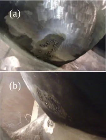
The traveling bubble cavitation causes loss of machine efficiency, loud acoustic noises, and erosion exclusively to the runner at the trailing edge of the blades on the suction side. Its characteristic modulation frequencies are the blade passing frequency and its harmonics.
The cloud cavitation can induce abnormal machine behavior and is very erosive. The typical damaged areas are near the leading edge of the runner blades or eventually the guide vanes. Its characteristic modulation frequencies are the vane passing frequency and its harmonics.
B. Cyclostationary Modeling of the SOI
Several random and deterministic phenomena govern the vibrational signal induced by erosive cavitation. The random
micro-phenomena are the collapses and impacts. The main deterministic macro-phenomena are the pressure fluctuations due to the rotor-stator interaction (RSI) and due to standing waves in the spiral case. Those deterministic phenomena modulate the rate and the amplitude of the collapses. The Computational Fluid Dynamics enables the hydrodynamic simulation of the macro phenomena, which can be modeled as periodic functions of the angular position θ of the turbine shaft. Thus, one can model the modulating signal of the traveling bubble cavitation as a Fourier series:
jbi B i i m B e
(2)where b is the number of runner blades, j is the imaginary unit, and Bi is the complex Fourier coefficient of the component of
machine order (MO) ib [9]. Similarly, the modulating signal generated by the cloud cavitation can be expressed as:
jvi C i i m C e
(3)where v is the number of guide vanes and Ci is the complex
Fourier coefficient of the component of MO iv. The MOs b,v, and multiples compose a set of key MOs. In addition, the model assumes that all modulating signals are non-negative for any θ.
The stationary vibrational signal (random carrier with constant variance) that is induced by the collapses can be modeled from the mechanical response to the impacts as:
, , * ,
B C B C B C
c
h n
(4)where cB(θ) is the vibrational signal due to bubble cavitation
only, cC(θ) is the vibrational signal due to cloud cavitation only
(already in angle domain), nB(θ) and nC(θ) are the acoustic
pressure random signals (similar to the Morozov model), hB(θ)
and hC(θ) are the impulse responses connecting the collapse(s)
point(s) to the external accelerometer location, and * denotes convolution. Both hB(θ) and hC(θ) are dependent on factors such
as multiple paths (including fluid and solid paths) and multiple resonant modes. The vibrational SOI due to each cavitation type is therefore a nonlinear function of the stationary carrier and of the modulating signal, which makes the variance a periodic function:
, , , , ,
SOI B C B C B C B C
x
f c
m
(5)Since the cloud cavitation damages the leading edge and the bubble cavitation damages the trailing edge of the runner blades, they have distinct mechanical transfer functions, and also distinct nonlinear functions for the vibrational SOI. Finally, the SOI is the sum of both:
SOI SOI B SOI C
x
x
x
(6)Since the variance of the SOI is angle dependent, it can be classified as a signal that exhibits [9] second-order cyclostationarity with respect to the angle domain. Moreover, one can conclude from (2) and (3) that the set of key MOs for the cavitation SOI is composed of b, v, and their integer multiples.
C. The Real Signal
Real vibrational signals are subject to contamination by various sources of noise, such as flow noise, electromagnetic interference from the generator, and friction. Another important source of vibrational interference is the electric generator itself [10].
Any vibrational signal is a sum of a periodic (deterministic) component and a residual (random) component. The cavitation SOI is part of the residual component. The residual part is also composed of the flow noise, the friction noise, and other noise sources, which are not dependent on the shaft angle. Thus, the SOI is the only part that exhibits second-order angle-cyclostationarity [9]:
CS1
CS2+
x
x
x
(7)In (7), xCS1(θ) is the deterministic or periodic part (which is
first-order angle-cyclostationary), xCS2+(θ) is the random
angle-cyclostationary part with orders greater than or equal to two (which includes the cavitation SOI and the stationary random noise), and η(θ) accounts for all non-cyclostationary and poly-periodic noise sources.
A real hydro turbine also shows some speed fluctuation (droop speed control). Angular re-sampling can correct this random speed fluctuation, although the time-domain excitation signals and frequency-domain transfer functions lose their meanings in the angle-domain. Nevertheless, the speed fluctuations are about 1%, which means little signal changes after re-sampling.
In order to build an estimator of the cavitation aggressiveness, only the power and the spectral similarity among the MO components of the SOI will be taken into account. Since different cavitation mechanisms induce vibrations through different mechanical transfer functions, it should be possible to distinguish MO components induced by different cavitation types. In addition, the pressure excitation signals are different, because cloud cavitation is subject to the harmonic cascading phenomenon [11].
III. METHODOLOGY
In order to detect erosive cavitation, the first step is to determine the key MOs set. In this work the authors recorded signals from two real turbines with b=11 rotor blades and v=24 guide vanes. The knowledge of b and v enabled the authors to synthesize a signal, which mimics the cavitation SOIs from the turbines and was useful to validate the processing algorithm. A. Acquisition of Real Signals
Signals from two identical Francis turbines, namely UG01 and UG02, were recorded. Each turbine-generator (TG) set has a nominal output power of 72 MW and shaft revolution frequency of 163.6 rpm (2.72 Hz). The generated voltage frequency is 60 Hz, thus each generator has 44 magnetic poles. Both turbines have track records showing low levels of erosion and were operating over 50,000 hours without maintenance. All generating units suffer from erosive traveling bubble cavitation
and cloud cavitation, as evidenced by visual inspection during the maintenance downtime, as shown in Fig. 1. For comparison purposes, UG01 was operating at 67% of its nominal capacity (48 MW) and UG02 was operating in the idle regime (0 MW). Both units were synchronized with the grid.
Two accelerometers manufactured by Rockwell Automation (model 9700A) picked up the vibrational signals. The turbine main bearings were inaccessible and non-invasive measurement was mandatory. Therefore, one sensor was installed on the turbine cover (immediately above the main turbine bearing), and the others were installed on the guide vane arms [2]. Due to the impossibility of screwing accelerometers directly at the turbine parts, steel mounting bases were carefully machined and fixed with cyanoacrylate glue, and the accelerometers were screwed into the bases.
Signal conditioners amplified and filtered the accelerometer signals, and the gain factor of 27 V/V was adopted. In order to minimize the interference from the power grid, batteries powered all sensors and signal conditioners. A 16-bit DAQ (model Agilent Technologies U2542A) connected to a portable computer recorded all signals at 100 kSamples/s per channel. The electric grid powered the recorder and the computer.
In order to measure the shaft angular position, an optical tacho signal (one pulse per shaft revolution) was recorded. Besides, the generator high-voltage output was reduced and recorded simultaneously. Since the generator is a synchronous machine with 44 poles, one expects 22 sinusoidal cycles per shaft revolution.
The U2542A recorded the two vibrational signals, the tacho signal, and the 60 Hz sinusoidal signal in a single multichannel binary file, which composed one signal set. Two signal sets were recorded from UG01 and one from UG02. Table I summarizes the main differences among all sets.
TABLEI SIGNAL SETS ACQUIRED Signal Set Generating Unit (power) Accelerometer 1 installed at Accelerometer 2 installed at Duration of recording 1 UG01 (48 MW)
Guide vane arm
5 Turbine cover 920 s
2 UG01
(48 MW)
Guide vane arm 5
Guide vane arm
4 875 s
3 UG02
a
(0 MW)
Guide vane arm 4
Guide vane arm
5 973 s
a This unit was at idle regime, but synchronous with the electric grid.
B. Signal Synthesis by Software
A (simplistic) synthetic signalx tˆ( )based on (2) to (7) was proposed to computer simulations. The nominal turbine speed is 2.7272 Hz, thus the expected modulation frequencies are 30 Hz for bubble cavitation and 65.45 Hz for cloud cavitation, besides their harmonics. A set of synthetic signals simulates 900 shaft revolutions with sampling rate at 100 kSamples/s.
For the acoustic excitations nB(θ(t)) and nC(θ(t)), two white
Gaussian random signals were generated [12]. Each one was filtered by a different band-pass IIR filter, which represents the impulse responses hB(θ(t)) and hC(θ(t)). The resultant signals
Two Fourier series simulated the turbine RSI, one for the bubble cavitation and the other for cloud cavitation, according to (8) and (9).
1 0,1
11
0,1
33
0.1
55
B
m
cos
cos
cos
(8)
1 0, 2
24
C
m
cos
(9) A nonlinear function simulates the modulation effect on bubble and cloud cavitation. The square root was introduced so that mB(θ) and mC(θ) modulates linearly the power (variance) ofthe random carriers as follows:
, , , , , ,
B C B C B C B C B C
f c
m
c
m
(10)The synthetic SOI for both cavitation types is:
ˆSOI B B C C
x
c
m
c
m
(11)Finally, a random process θ(t) simulated the droop speed control of 1%. Based on θ(t), the simulated angle-domain signal can be represented by a time-domain signal. A Gaussian white noise ηS(t) with power spectral density of 3∙10-7 V2/Hz, and a
tonal noise ηT(t) (two sinusoidal components at 30 and 40 kHz
and power of 7.5∙10-2 V2) were added. Therefore, the complete
mathematical model for the synthetic SOI is:
ˆ
ˆ
ˆ ˆSOI T S
x t x
t
t
t (12) C. Cavitation aggressiveness estimator based on SOI powerThe processing starts with the conversion of the recorded signals from time-domain into angle-domain by angular re-sampling (order tracking). The re-sampling is carried out by sinc interpolation [13] and the speed fluctuation is less than 1% for a 15-minute interval. Signals are oversampled so that every shaft turn has the same number L of samples, which is an integer multiple of N, where N is a power of two. Such L feature is essential for the next step, which employs analysis windows of length N. This oversampling, in the case of UG01 and UG02, corresponds to L=45056 samples per turn and to the new sampling rate of 122880 samples/s. 1) Removal of the First-order Cyclostationary Part
Let x[n] be the angular domain re-sampled signal from an arbitrary sensor. The removal of the first-order cyclostationary [9] part is done by subtracting the synchronous average (SA), which is an estimator of the deterministic part of the signal:
1 1 0 1K CS k x n x kL m K
(13)where K is the number of recorded shaft turns and m is the remainder of the division between n and L(note that n=kL+m). The residual part of the signal is the difference:
1
CS2+
r CS
x n x n x n x n
n (14) where xCS2+[n] is the cyclostationary part (with order ≥ 2) of thediscrete signal, and η[n] accounts for all other components with different characteristics. Therefore, the cavitation SOI is part of the residual signal.
2) Enhancement of the Pure Second-order Cyclostationary Part
In order to reduce the noise term η[n], the averaged instantaneous power spectrum (AIPS) of the residual signal is
computed [14]. The angle-frequency representation is required for posterior MO-frequency representation. Additionally, the AIPS merges some advantages from the SA and from the time-frequency (or angle-time-frequency) representation.
The AIPS calculation is based on the FFT of the residual signal: the residual discrete signal xr[n] is divided into K
segments of L samples, where K is the number of complete revolutions of the shaft during the recording interval. For each segment, an N-long analysis window w[n] is introduced and shifted along the signal by steps of R samples (R<N). The shifted analysis window wN[n]=w[n-iR] (which is typically a
Hanning window) effectively selects a chunk of the K-th segment around time samples n=iR,...,iR+N-1, and the Fast Fourier Transform (FFT) of the product xr[n]wN[n] is computed.
The resultant complex matrix is known as the discrete Short Time Fourier Transform (STFT) of the signal. The instantaneous power spectrum (IPS) of the K-th segment is:
2 1 2 1 , n iR iR N j h N K r N n iR IPS i h x n w n e
(15)where i is the discrete angle domain variable, and h is the discrete spectral frequency variable. The second-order non-linear operation makes possible the discrimination of second-order cyclostationary signals. N=512 was adopted for UG01 and UG02. This criterion leads to an angular resolution that is high enough to discriminate events due to a single blade or guide vane. Finally, the AIPS considers all revolutions, and it is computed by taking the average of the IPSs for each revolution:
Fig. 1. Typical cavitation damage patterns. (a) Damage due to traveling bubble cavitation. (b) Damage due to cloud cavitation.
1 0 1 , , K k k AIPS i h IPS i h K
(16)3) Discrimination of Machine Order Components
The pure second-order cyclostationary signal can be analyzed using suitable cyclostationary tools, namely the CMS and the CMC. The CMS highlights any amplitude modulation, and reveals the periodicities hidden in the random signals. In this work, the CMS is obtained by computing the FFT of the AIPS, which transforms angle domain into MO domain:
1 2 1 0 1 , , i I j a I x i CMS a h AIPS i h e I
(17)where a is the MO domain discrete variable and CMSx[0,f] is an
estimator of the power spectrum (PS) of the vibrational signal, which shows only the stationary components. Finally, the CMC normalizes the average power spectrum as follows:
, , 0, x x x CMS a h CMC a h CMS h (18)The CMC is a complex matrix, and the meaning of the magnitude of each element CMCx[a,h] is the degree of
cyclostationarity. The image formed by |CMCx[a,h]| constitutes
a visual indicator of the presence of cyclostationarity. 4) Estimator of the Cavitation Aggressiveness
The image formed by |CMSx[a,h]| constitutes a representation
of power distributed among spectral frequencies and MO components, thus the cavitation SOI should appear as vertical lines at the key MOs set. Moreover, these vertical lines are composed of random dots and dashes, and their patterns depend on the acoustic excitation sources and on the mechanical transfer functions up to the sensor.
The estimator of bubble cavitation aggressiveness is built by taking the component of MO b as a reference of spectral distribution and computing its power. The powers of the components of MO mb (m is an integer>1) are also accumulated if there is spectral similarity with the reference component. This similarity is evaluated by the Pearson product-moment correlation coefficient (PPMCC) computed between the two discrete spectral power distributions:
,
B x
m h
P
CMS amb h (19)The estimator for the cloud cavitation aggressiveness is built in a similar manner, but the reference is the component of MO v:
,
C x
m h
P
CMS amv h (20)Finally, both PB and PC are divided by the power of the
stationary component (a=0), which reveals the percentage of power that is modulated due to the cavitation mechanisms:
, B%,C% 0, B C x h P P CMS h
(21)D. Development of a cyclostationarity-based application specific software
In order to monitor the erosive cavitation in turbines, the authors developed a software that performs all the processing steps described in Section III.C. The software plots the image formed by |CMCx[a,h]| and makes a concise text report, which
contains the cavitation aggressiveness estimators of traveling bubble and cloud cavitation.
IV. RESULTS AND DISCUSSIONS
The developed software processed the synthetic signal set along with all signal sets from the turbines, and the computed estimators are summarized in Table II. Regarding the PPMCC threshold, the value of 0.6 was chosen, which yielded the best discrimination among different cavitation mechanisms and second-order cyclostationary interfering signals.
A. Synthetic Signal Set
Two synthetic signalsx tˆ ( )1 andx tˆ ( )2 were implemented, and they compose the synthetic signal set. Both signals have a stationary additive white Gaussian noise with power equal to 0.015 V2. Additionally, the signal
2
ˆ ( )
x t has two tonal noises with powers equal to 0.075 V2. The sum of the powers of the
bubble and cloud cavitation SOIs is 0.070 V2. The graphics of
CMCs magnitudes are shown in Fig. 2. There are three continuous vertical lines representing traveling bubble cavitation at MOs 11, 33, and 55. There is also one continuous line representing cloud cavitation at MO 24. The tonal noises at 30 and 40 kHz have little influence on the results.
According to (8)and (9), PB accounts for 30% of cB(θ) power,
and PC accounts for 20% of cC(θ) power. The powers of cB(θ)
and cC(θ) are 0.030 V2 and 0.040 V2 respectively, which means
that conventional true values of PB and PC are respectively
0.009 V2 and 0.008 V2.
For signalx tˆ ( )1 the measured values for PB and PC show
relative measurement errors of -2.67% and -3.75%. In addition, the proposed method detected the power of the SOIs separately, even under a significant stationary noise. For signalx tˆ ( )2 the results in Table II and Fig. 2 show that the tonal noise has little influence on the detection and separation of the cavitation SOIs powers.
B. Results on UG01
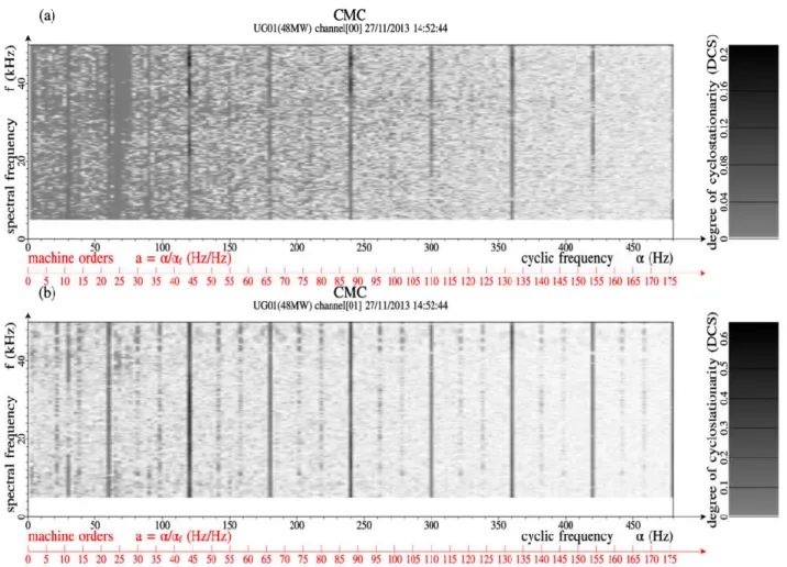
The CMC magnitudes computed from the vibrational signal set 1 are shown in Fig. 3. The AIPS rows corresponding to spectral frequencies below 5 kHz were not processed, because signals below 5 kHz are too noisy due to machine noise sources. There are not only discontinuous lines at the key MOs set, but also strong interfering components at MOs 22 (60 Hz), 44 (120 Hz), and multiples. The CMC magnitudes computed from the vibrational signal set 2 are shown in Fig. 4. The same expected MO components for the bubble and cloud cavitation are present. The interfering components at MOs 22, 44 and multiples are even stronger than in signal set 1.
Fig. 2. CMC computed from synthetic signals: (a) cavitation SOIs plus white Gaussian noise. (b) cavitation SOIs plus white Gaussian noise and tonal noises.
The results presented in Fig. 3 show the traveling bubble cavitation SOI at MOs 11, 33, 55 (weak), and 77 (very weak). There is also a component at MO 24, a signature of cloud cavitation. Additionally, there is a component at MO 25 Fig. 3 a only), which suggests the presence of a Von Kármán [15] vortex shedding that interferes with the cloud cavitation. Fig. 4 shows results from signal set 2 that are consistent with the ones shown in Fig. 3 a. The corresponding entries in Table II corroborate the results for the aggressiveness of both bubble and cloud cavitation. The detection of bubble cavitation using a sensor near the shaft was more feasible, but rendered the detection of Von Kámán vortex cavitation impossible.
The authors concluded that the strong noise components at MOs 22, 44, and multiples are from the electric generator, due to the fact that the magnetic materials shows Barkhausen noise and magnetostriction. Both effects compose a source of mechanical Barkhausen noise [16], which is modulated at the electric grid frequency and at the magnetic pole passing frequency. This modulated noise is not intermittent but characteristic cavitation signals are intermittent, unless cavitation is at developed stage. Unfortunately, these components may mask part of the traveling bubble cavitation SOI. Therefore, its estimator may be somehow biased. C. Results on UG02
The CMC magnitudes computed from the vibrational signal
set 3 are shown in Fig. 5. The absence of lines at the key MOs is noteworthy. Table II reveals that the measured PB and PC are
one order of magnitude lower than the ones obtained from UG01, despite the total power remains in the same order of magnitude. One can conclude that both bubble and cloud cavitation are absent in UG02, despite the methodology detected the noise from the generator.
V. CONCLUSIONS
The proposed method is suitable to detect the cavitation and estimate its aggressiveness, even under strong noise. Moreover, different cavitation mechanisms produce not only components with different machine orders (modulating signal), but also with different spectral compositions (carrier). Each cavitation type is characterized by a unique combination of random carrier and modulating signal.
The CMC, together with the extracted powers of the cavitation SOIs, enables the diagnostic and identification of cavitation in hydro turbines with low levels of cavitation aggressiveness. Although it is not exactly a real time signal processing such as DEMON, this methodology is not empirical and there is no information loss due to band pass filtering. Moreover, the proposed method is non-invasive and does not interfere with turbine operation.
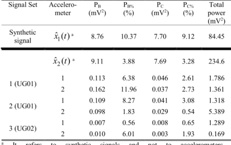
TABLEII
COMPUTED ESTIMATORS OF CAVITATION AGGRESSIVENESS Signal Set
Accelero-meter PB (mV2) PB% (%) PC (mV2) PC% (%) Total power (mV2) Synthetic signal x tˆ ( )1 a 8.76 10.37 7.70 9.12 84.45 2 ˆ ( ) x t a 9.11 3.88 7.69 3.28 234.6 1 (UG01) 1 0.113 6.38 0.046 2.61 1.786 2 0.162 11.96 0.037 2.73 1.361 2 (UG01) 1 0.109 8.27 0.041 3.08 1.318 2 0.098 1.83 0.029 0.54 5.389 3 (UG02) 1 0.007 0.56 0.008 0.65 1.289 2 0.010 6.01 0.003 1.93 0.169
a It refers to synthetic signals and not to accelerometers.
REFERENCES
[1] K.A. MØRCH, Cavitation Nuclei: Experiments and Theory, Journal of Hydrodynamics, Ser. B. 21 (2009) 176–189. doi:10.1016/S1001-6058(08)60135-3.
[2] X. Escaler, E. Egusquiza, M. Farhat, F. Avellan, M. Coussirat, Detection of cavitation in hydraulic turbines, Mechanical Systems and Signal Processing. 20 (2006) 983–1007. doi:10.1016/j.ymssp.2004.08.006. [3] J.-P. Franc, J.-M. Michel, Cavitation erosion research in France: the state
of the art, Journal of Marine Science and Technology. 2 (1997) 233–244. doi:10.1007/BF02491530.
[4] M. Farhat, P. Bourdon, P. Lavigne, Some hydro Quebec experiences on the vibratory approach for cavitation monitoring, in: Proceedings of Modelling, Testing and Monitoring Conference, Lausanne, Switzerland, 1996: pp. 151–161.
[5] M.K. De, F.G. Hammitt, New Method for Monitoring and Correlating Cavitation Noise to Erosion Capability, Journal of Fluids Engineering. 104 (1982) 434. doi:10.1115/1.3241876.
[6] B. Bajic, Methods for vibro-acoustic diagnostics of turbine cavitation, Journal of Hydraulic Research. 41 (2003) 87–96. doi:10.1080/00221680309499932.
[7] J. Antoni, D. Hanson, Detection of Propeller Noise under Low SNR with the Cyclic Modulation Coherence (CMC), in: 10ème Congrès Français d’Acoustique, Société Française d’Acoustique, Lyon, France, 2010: pp. 12–16.
[8] V.P. Morozov, Cavitation noise as a train of sound pulses generated at random times, SOVIET PHYSICS ACOUSTICS. (1969) 361–365. [9] J. Antoni, Cyclostationarity by examples, Mechanical Systems and Signal
Processing. 23 (2009) 987–1036. doi:10.1016/j.ymssp.2008.10.010. [10] R. Oliquino, S. Islam, H. Eren, Effects of Types of Faults on Generator
Vibration Signatures, in: Australasian Universities Power Engineering Conference, 2003: pp. 1–6.
[11] S. Kumar, C. Brennen, Harmonic cascading in bubble clouds, (1992). [12] J. Antoni, D. Hanson, Detection of Surface Ships From Interception of
Cyclostationary Signature With the Cyclic Modulation Coherence, IEEE Journal of Oceanic Engineering. 37 (2012) 478–493. doi:10.1109/JOE.2012.2195852.
[13] J.O. Smith, P. Gossett, A flexible sampling-rate conversion method, in: ICASSP ’84. IEEE International Conference on Acoustics, Speech, and Signal Processing, Institute of Electrical and Electronics Engineers, 1984: pp. 112–115. doi:10.1109/ICASSP.1984.1172555.
[14] J. Urbanek, T. Barszcz, J. Antoni, Time–frequency approach to extraction of selected second-order cyclostationary vibration components for varying operational conditions, Measurement. 46 (2013) 1454–1463. doi:10.1016/j.measurement.2012.11.042.
[15] P. Ausoni, M. Farhat, X. Escaler, E. Egusquiza, F. Avellan, Cavitation Influence on von Kármán Vortex Shedding and Induced Hydrofoil Vibrations, Journal of Fluids Engineering. 129 (2007) 966. doi:10.1115/1.2746907.
[16] P. Maciakowski, B. Augustyniak, L. Piotrowski, M. Chmielewski, Measurements of the mechanical Barkhausen noise in ferromagnetic steels, in: PROCEEDINGS OF ELECTROTECHNICAL INSTITUTE, 2012: pp. 221–228.
Rafael Linhares Marinho received the B.Sc. and M.Sc. degrees in electrical engineering from the Universidade Federal do Rio de Janeiro, Rio de Janeiro, Brazil, in 2001 and 2005 respectively. Since 2009 he has teached at Instituto Federal do Rio de Janeiro. His research interests include analog integrated circuit design, radio frequency circuits, industrial instrumentation, and automation.
Fernando Antônio Pinto Barúqui received the B.Sc., M.Sc, and D.Sc. degrees in electrical engineering from the Universidade Federal do Rio de Janeiro, Rio de Janeiro, Brazil, in 1987, 1990, and 1999, respectively. Since 1990, he has been an Associate Professor with the Department of Electronic Engineering, and with the Electrical Engineering Program (PEE/COPPE), Universidade Federal do Rio de Janeiro. His research interests are signal processing and integrated circuit design for mixed-signal applications.