Rodrigo M. S. de Oliveira, Jonathas F. M. Modesto, Victor Dmitriev, Fernando S.
Brasil, Paulo R. M. de Vilhena.
Federal University of Pará (UFPA) - Rua Augusto Corrêa, 01, Belém, Pará, Brazil – CEP 66075-110. E-mails: [email protected], [email protected], [email protected], [email protected],
Abstract — A methodology based on spectral analysis for localization of multiple partial discharges in dielectric region of hydro-generator coils is proposed. This pinpointing of multiple discharges aims to provide means for performing diagnosis of insulating regions of the coil. A numerical model of the structure was developed by using the finite-difference time-domain method (FDTD-3D) to solve Maxwell’s equations. Transient voltage associated with partial discharges that occurs at different positions of the coil is calculated at specific point and its spectrum is used to perform the diagnosis. In 90% of simulations, accurate estimates of simultaneous discharges location were obtained. Physical phenomena allowing the development of the methodology are assessed numerically and experimentally. Finally, a localized artificial PD injection schema is proposed and used for validating our numerical results and physical analysis.
Index Terms — Hydro-generator coils, method of diagnosis, partial discharges, spectral analysis.
I. INTRODUCTION
The quality of the insulation in high voltage equipment is a key issue to keep them functioning
[1-12]. Electric field of high levels in this equipment produces degradation of insulating parts of the
apparatus. This degradation involves the formation of heterogeneities in the insulating material so that
high amplitude electric field inside these localized heterogeneities gives rise to the partial discharges
(PDs). Many discharges can occur in a single working cycle of the generator and the dielectric
insulation may be compromised. Such discharges have been studied [3-5] and it was verified that the
transient fields produced by them may be used to diagnose the state of isolation.
During the last 10-15 years, different mathematical methods have been proposed to localize
discharges in high voltage equipment [3-7]. Neural networks techniques were used in [3] to identify
Spectral Method for Localization of Multiple
Partial Discharges in Dielectric Insulation of
Hydro
-
Generator Coils: Simulation and
patterns relative to PDs. In that work, experiments were performed by using especially constructed
bars to characterize situations where different types of discharges (lamination, winding and slotting)
are produced. In [4], fuzzy logic was applied to perform PD transient pattern analysis in transformers.
In [5], the authors used wavelet transforms to accomplish discharge pinpointing. In [6], a technique
called Intech was presented which allows one to identify more precisely the region of the generator
producing the discharges. In [8], the particle swarm optimization (PSO) method was applied for
diagnosis of power transformers. Several measurement techniques have also been presented. In [9],
optical sensors were used to perform the localization of single and multiple discharges in high voltage
equipment. In [7] and [10], acoustic measurements combined with different electrical methods were
used to localize discharges in transformers.
In this paper we present a new technique for localization of multiple PDs by using spectra of
transient voltages registered at a single point of a hydro-generator coil. The fields producing the
voltages originate at the PDs occurrence loci. In short, the technique consists of mapping frequencies
associated with maxima and minima of the signals’ spectrum received by a sensor and to relate them to discharges occurrence positions. This approach is justified by the natural resonances [13,14]
produced by the investigated structure [15], which are also functions of the positions of the
electromagnetic excitations. The resonances are investigated both numerically and experimentally.
The main advantage of this methodology is a possibility to identify multiple simultaneous
discharges by using the superposition principle, including those occurring in distinct coils. The
effectiveness of the proposed method is confirmed by numerical analysis. The developed
finite-difference time-domain (FDTD-3D) simulator [16] is validated for this problem by reproducing
numerically experimental setups available in literature. Experimental investigation is also conducted
in this paper. A controlled local PD injection schema is proposed and validated by comparing
experimental and numerical results.
II. PROBLEM DEFINITION AND PROPOSED TECHNIQUE
A. Partial Discharges
Partial discharges are electrical micro-discharges which occur within an insulating structure when it
is subjected to high intensity electric fields. These fields break the dielectric strength at specific
regions. Thus, PDs can only partially break down the insulation between conductors [11].
Physically, the partial discharges are characterized by an ionization process in a gaseous medium
within the dielectric material caused by the aforementioned intense and localized electric field. This
process produces specific physical phenomena, such as light flashes, acoustic noise, temperature
gradients, chemical reactions and conducted and radiated electromagnetic pulses [3-11].
B. Physics of the Problem: Resonance Analysis
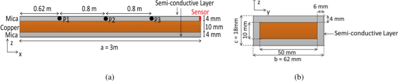
In order to verify basic physical aspects of the problem, a rectangular bar was modeled (Fig. 1) with
by partial discharges taking place at different points in the insulation layer. The modeled bar is 3 m
long (Fig. 1a) and it is formed by three layers: inner metal bar (copper), which is surrounded by a
dielectric layer (mica), that in turn is coated with a semi-conductive outer layer (Fig. 1b).
(a) (b)
Fig. 1. Sections of the rectangular bar: (a) longitudinal and (b) transversal.
Separate occurrences of z-polarized partial discharges were simulated at three points (P1, P2 and
P3) of the FDTD-3D model of the bar (Fig. 1) by excitation of Ez component and the induced
transient voltage is registered by a sensor at the point indicated in Fig. 1a. Several simulations were
performed by changing the following parameters: electrical permittivity and conductivity of mica and
rise time of the excitation signal.
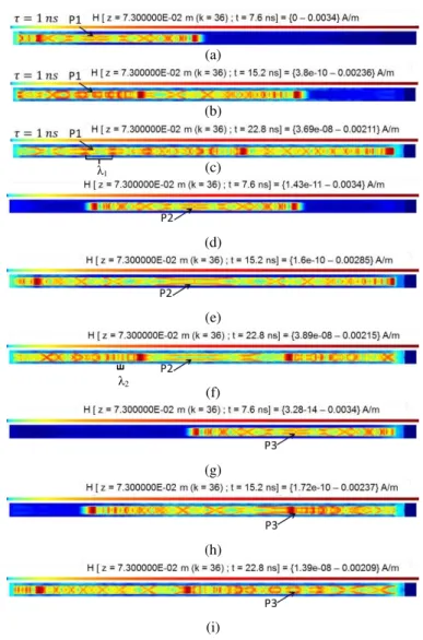
For the best field visualization, Fig. 2 shows the magnetic field (instead of electric field)
propagation produced by partial discharges simulated at P1, P2 and P3 for three different instants. The
dielectric parameters are �� = 5.4, σ = 0.10394 mS/m and �� = 1 [13,17]. It is possible to observe
clearly in Fig. 2 that particular wavelengths are produced as function of PD position, such as λ1 and
λ2, which are indicated in Figs 2c and 2f for t = 0.0228 µs for better illustration of this effect. This takes place due to field reflections at the bar’s extremities and to the distances involved in this
electrodynamic process (from PD position to bar ends) producing natural electromagnetic resonances.
Additional resonances emerge due to field reflections at the metallic parts of the bar.
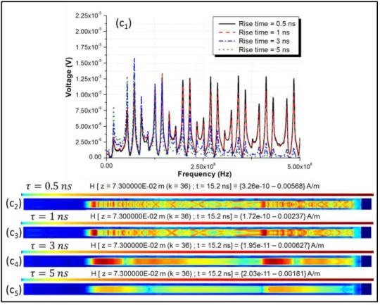
The first parameter studied is the rise time � of the discharge pulse. Pulses with rise time of 0.5 ns,
1 ns, 3 ns and 5 ns [12] were simulated. For this analysis, mica insulator was modeled by using the
parameters �� = 5.4, σ = 0.10394 mS/m and �� = 1 [13,17]. It was found out that maxima and minima
spectral loci, in essence, depend on the structure itself and, of course, on the PD’s position, since they
remain unchanged when � is modified (Figs. 3(a1), 3(b1) and 3(c1)). This is associated with the field
reflections at the bar ends as discussed above. Different wavelengths for this case are observable in
the field distributions of Figs.3(a2)-(a5), Figs.3(b2)-(b5) and Figs.3(c2)-(c5). It should be noted that for
rise times of 0.5 ns and 1.0 ns, the signal strength received by the sensor carries energy in the high
frequency range of the analyzed spectrum. For this reason, the signal amplitudes are higher for
frequencies from approximately 600 MHz. Notice that the frequencies points at which the maxima
and minima occur in the spectrum are preserved as long as the PD pulse contains energy in the
analyzed spectral range.
4 mm
4 mm 10 mm Mica
Mica Copper
a = 3m x
z
Semi-conductive Layer Sensor
P1 P2 P3
(a)
(b)
(c)
(d)
(e)
(f)
(g)
(h)
(i)
Fig. 2. Visualization of magnetic field propagation for PD taking place at (a) P1 for t = 0.0076 �s, (b) P1 for t = 0.0152 �s, (c) P1 for t = 0.0228 �s, (d) P2 for t = 0.0076 �s, (e) P2 for t = 0.0152 �s, (f) P2 for t = 0.0228 �s, (g) P3 for t = 0.0076 �s, (h) P3 for t = 0.0152 �s and (i) P3 for t = 0.0228 �s. The dielectric parameters are ��= 5.4, σ = 1.0394 ×10⁻⁴ S/m and �� =1.
The effect of the electrical conductivity � of the dielectric was also numerically investigated. For
each excitation point (P1, P2 and P3), three simulations were performed with different values of �
(~5.2×10⁻⁵, 1.04×10⁻⁴ and 2.07×10⁻⁴ S/m) [17]. The parameters �� and �� were fixed to 5.4 and 1,
respectively.
It has been observed, as expected, that frequencies where maxima and minima occur in the
spectrum do not change when � is altered. The modifications observed in spectra (Fig. 4) as function
of � are associated to spectral amplitudes only, i.e. with increasing �, currents tend to be superficial
and internal electric field is reduced according to the well-known skin effect [14]. Fig. 4 shows the
comparison among the spectra of the received signal for excitation at P2, illustrating the
aforementioned effect. Excitation at P1, P3 or at any other point presents the same physical behavior. λ1
(a)
(c)
Fig. 3. Comparison of the spectra of the received signals with for different rise times: (a) for partial discharge placed at P1, (b) at P2 and (c) at P3.
Fig. 4. Comparison of spectra of received signals for different values of � for PD excitation at P2.
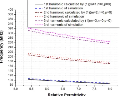
Finally, the spectral effects of relative electrical permittivity of mica were evaluated. The
simulation of the partial discharge occurring at P1 (Fig. 1a) was repeated. However, �� of dielectric
was set to various values between 5.4 and 8.0 (as it is specified for mica in [13]).
Considering the bar of Fig. 1 as a waveguide, it was verified analytically the occurrence of
resonance frequencies �� in the spectral range from 80 to 400 MHz. For purposes of validation of
V
o
lt
a
g
e
(
V
numerical solutions, the resonance frequencies of the bar were calculated analytically using equation
(1) [14]. The comparison of frequencies calculated by (1) and by FDTD simulation is shown in Fig. 5.
According to [14], resonance frequencies can be obtained by the expression
��=�
′
2 √[ ]
2
+ [ ]2+ [�]2, (1)
where �′ is the propagation speed of signal in mica, which is a function of ��. The dimensions of
waveguide are expressed by a, b and c (Fig. 1) and m, n and p are integers. It is observed in Fig. 5 that
the numerical and analytical results are in a good agreement. Notice that because the goal is to locate
the PD along x (Fig. 1a), longitudinal resonances are of greater interest. Thus, n and p are set to zero.
Fig. 5. Comparison of resonant frequencies calculated using (1) and frequencies obtained via FDTD simulation.
C. Problem Description and Numerical Modeling
The design schematics of a synchronous generator winding of 48 salient poles were provided by
Eletronorte. The machine has the following nominal specifications: power of 30.4 MW, voltage of
13200 V, operating range of ± 5%, current of 1330A oscillating at 60 Hz, and power factor of 0.95.
By using the equipment’s project files [15] (Fig. 6a), it was possible to obtain a detailed FDTD model of a stator coil, which is represented by Fig. 6b. A specific computational routine was developed to
export these geometric data to the FDTD simulator developed in [16], called SAGS, which has been
adapted for simulating PDs. Numerical validation of this software for the present problem, which was
performed by comparing results with literature data, is given in Appendix (Sections A and B).
The FDTD numerical model of the bar is formed by three layers: inner metal structure, which is
surrounded by a dielectric layer, which in turn is coated with a metallic layer (outer), as illustrated by
Fig. 6b. The dielectric layer (mica) is characterized by (average) parameters �� = , σ = 0.10394
mS/m and �� = [14]. Metallic parts are considered to be copper (�� = , � = 5. × 7 S/m and
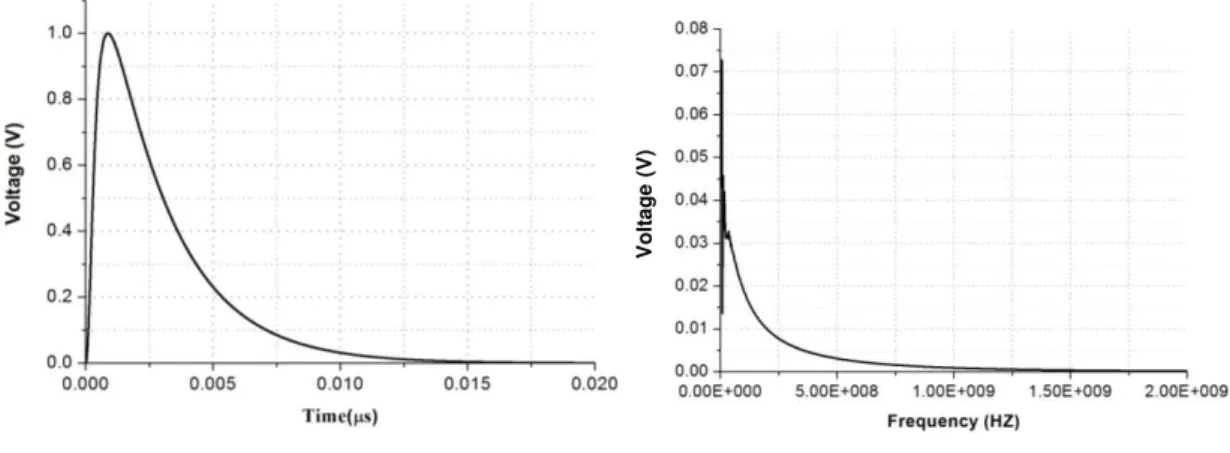
the waveform of the voltage source used to model the discharges as a function of time and Fig. 7b
illustrates its spectrum. As far as the maximum significant frequency of the pulse is approximately 1
GHz (Fig. 7b), the maximum edge allowed for Yee’s cell (the FDTD spatial discretization element) for reducing numerical dispersion to acceptable levels [19] is Δmax = 30 mm. Thus, the edges of every
Yee cell in the grid measures Δx = Δy = Δz = Δ = 2 mm, ensuring uniform spatial wave sampling for
directions x, y and z. The rectangular FDTD grid, created to represent space and the analyzed
structures, contains 848 × 254 × 165 identical cells [19].
(a) (b)
Fig. 6. (a) 3D view of the hydro-generator coil in SolidWorks®; (b) inner structure of the model represented by the SAGS [16] FDTD simulator.
D. Spectral Technique for Diagnosing the Coils
As described previously, several partial discharges at different locations may occur concurrently in
a given coil. Thus, pairs of simultaneous discharges were simulated, occurring in the quadrants shown
in Fig. 8. Discharges produced in a single quadrant were also considered. The signals from partial
discharges propagate through the structure and suffer multiple reflections. The signals have their
propagation velocities reduced when compared to the speed of light in vacuum due to the relative
permittivity of the insulation. Furthermore, signals are attenuated due to the low electrical
conductivity of mica and due to natural expansion of wave. For this reason, transient signals received
by the sensors (Fig. 8) are strongly dependent on the discharge(s) position.
Considering that each pair of transmitter (PD) and receiver (sensor S) represents a unique
propagation channel, it is verified that every part of the coil produces a unique spectral pattern in
which local maxima and minima characterize a given spatial region due to produced specific
resonances (this physical aspect is verified experimentally in Appendix, Section C). With this
information in mind, a computer algorithm (Fig. 9) was developed and implemented for identifying
the frequencies at which local maxima and minima occur in the spectral functions. A database was
elaborated, containing such resonance frequencies and the coordinates L of the coil associated with
transmission points and with a specific receiver. The database is used to estimate the region(s) where
discharges arise (Fig. 5).
Once the database was available, two simultaneous discharges, placed at different positions, were
simulated and the Fourier transforms of the signals captured by the sensor were calculated (Fig. 9).
Due to the superposition principle for Maxwell’s equations and for the Fourier transform, when
multiple discharges at different points occur simultaneously, their individual spectra are naturally
added up (see Fig.11). This observation allows one to search for groups of resonances, in the spectrum
concerning simultaneous PDs, which characterize the individual contribution of a specific PD
occurring at a definite position.
(a) (b)
Fig. 7. (a) Normalized waveform of excitation source used for model partial discharges, (b) excitation source spectrum.
(a)
(b)
Figure 8. (a) Cross section of bar and relation of L with positions in structure regions; (b) L variable in a one-dimensional coordinates system.
Of course, specific resonance information can be modified (or even canceled) by the composition of
the multiple discharge spectra. However, this can be treated by defining a probability of occurrence of
a PD in a specific position of the structure. This probability p[L] can be calculated by counting the
total number of resonances C[L] stored in database for a PD flashing at position L which are also
present in the measured spectrum (result of an arbitrary quantity of occurring PDs). Mathematically,
we have the expression
%, 100 ] [ ] [ ] [ L n L C L p (2)
where n [L] is the total number of resonances present in the database for a discharge occurring at L.
This idea is algorithmically detailed by the flowchart in Fig. 9. The algorithm is then repeated for
V o lt a g e ( V )
L = 0 L = 0,76 m L = 1,88 m
L = 2,73 m
L= 0
L= 0.76 m
L= 1.88 m
L= 2.73 m
Q1 Q2
Q3
Q4
S
L= 0 L= 0.76 m L= 1.88 m L= 2.73 m L= 3.85 m
other values of L and a map of statistical chances for discharge localization is created.
Each modeled pair of partial discharge was indexed by an integer number. For purposes of
illustration, Fig. 10b shows the points excited by partial discharges for simulations with indices 5 and
161.
Fig. 9. Algorithm for proposed technique for a fixed value of L.
(a)
(b)
Fig. 10. (a) Visualization of electric field propagation at t = 0.191 µs (xy-plane that intersects the bar’s centroid); (b) sensor location and simultaneous discharges locations of simulations 5 and 161.
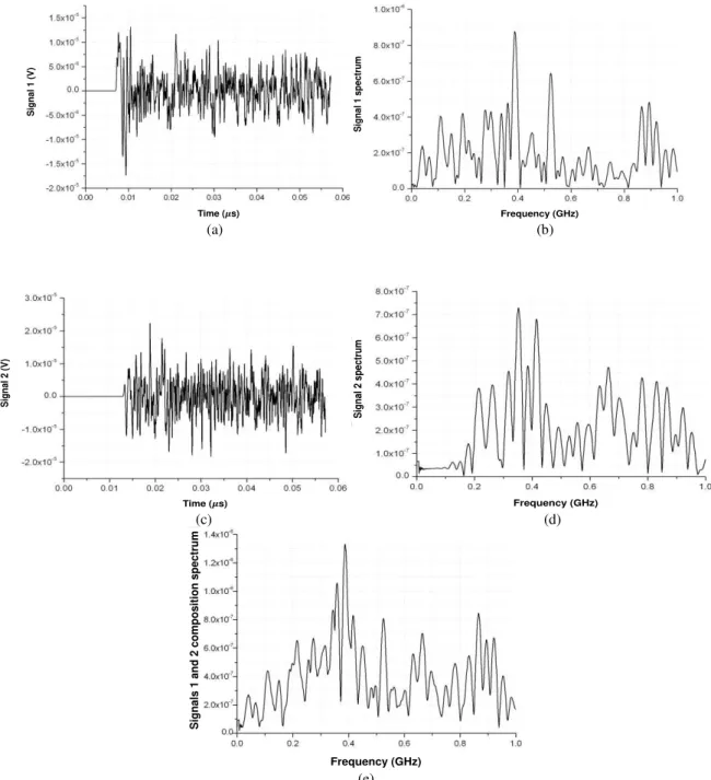
The transient signals recorded by the S sensor for discharges 1 and 2 of simulation 161 (see Fig.
10b), occurring in dielectric region, are illustrated in Figs. 11a and 11c. Their spectra are shown
respectively by Fig. 11b and 11d. As established by the superposition principle, the simultaneous
occurrence of two pulses generates linear combination of the two temporal signals and of their spectra
(Fig. 11e). It is noted, by comparing Figs. 11b, 11d and 11e, that most local minimum and maxima
LOCATION OF THE FREQUENCIES OF OCCURRENCE OF LOCAL MAXIMA AND
MINIMA
GENERATION OF A LIST WITH THE FREQUENCIES OF
MAXIMUM AND MINIMUM.
fiWITH i =1,2,..., n
IS THE FREQUENCY fi
(WITH MARGIN 0,3%) FOUND IN
REGISTRIES? COMPARISON OF
FREQUENCY fi
WITH FREQUENCIES OF REGISTERED PATTERNS IN DATABASE IGNORED FREQUENCY NO YES
i =n ?
NO
p[L]= p[L] + 1 YES
CALCULATE
p[L] = ( p[L] /n ) 100
TRANSIENT SIGNAL FOURIER TRANSFORM CALCULATION OF TRANSIENT SIGNAL
.
Sensor Simultaneous discharges of simulation 5.
.
Simultaneous discharges of simulation 161
seen in Figs. 11b and 11d are preserved in the graph of Fig. 11e, enabling the identification of the
several discharges. Additionally, it is noteworthy that this is true even when the discharges do not
initiate exactly at the same moment, because the magnitude of the Fourier transform is being
considered and its phase is neglected.
(a) (b)
(c) (d)
(e)
Fig. 11. Voltage signals of simulation 161 registered by the sensor S. For discharge 1, we have: (a) the registered transient signal and (b) its frequency spectrum. For discharge 2, we have: (c) the registered transient signal and (d) its frequency spectrum. The simultaneous occurrence of discharges 1 and 2 produces the spectrum given in (e).
III. RESULTS
A. Localization of Multiples Discharges in a Single Coil
Several simulations of concurrent partial discharges were performed initially for a single
hydro-generator stator coil. For illustrative purposes, the electric field distribution on a horizontal plane
Time ( s)
Sig
nal
1 (V)
Frequency (GHz)
Sig
nal
1 s
pec
trum
Time ( s)
Sig
nal
2 (V)
Frequency (GHz)
Sig
nal
2 s
pec
trum
Frequency (GHz)
Si
gnals
1
and 2
composi
tion
spect
(parallel to x-y plane) crossing the center of coil it is shown in Fig. 10a. Reddish colors mean higher
field stress (intensity) and colors close to blue identify smaller magnitudes.
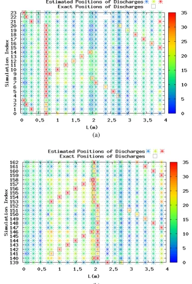
Fig. 12 shows the results obtained by using the diagnostic method (see Fig. 9) proposed in this
work. The horizontal axis in Fig. 12 represents L (m), which is defined in Fig. 8, and the vertical axis
shows the index of simulations. Thus, statistical results for a given numerical experiment are
presented in the corresponding line of the maps in Fig. 12. The definition of L is given in Fig. 8.
(a)
(b)
Fig. 12. Statistics of discharge localization for a single coil for several simulation indices: (a) 0 t o23 and (b) 139 to 162.
It was performed a total of 231 numerical experiments distinguished by different positions of partial
discharges excited along L (from zero to 3.87 m). Gray rectangles indicate the exact (known)
locations of partial discharges excited in each simulation. Noticeably, during laboratorial experiments
these exact locations are unknown and can be estimated by the proposed methodology. Aiming the
statistical PD pinpointing, the color bar in Fig. 12 maps values of p[L]. As discussed previously, p[L]
is proportional to the probability of PD occurrence at a specific point in the bar specified by L (Fig. 8).
Consequently, for a given simulation, the statistical assessment is performed by calculating p for
every considered value of L, obtaining the changes of finding a PD source throughout the coil. This
positions on the bar are marked with a sequence of colored crosses in each line of Figs. 12a and 12b
and the color of a given cross indicates the possibility of finding a PD for each considered value of L.
Shades of blue or green indicates lower chances of finding a PD source. Shades of yellow and red
suggest higher possibilities of correct PD pinpointing.
For exemplifying, consider results of simulation 10, in Fig. 12a. We see that there is a coincidence
of positions among gray rectangles and red crosses. In this case, both PD sources simulated were
accurately localized at L = 0.25 m and L = 1.0 m. This accuracy is seen for most of the tested cases.
This is not the case for simulation 21, in which PDs were excited at L = 0.25 m and L = 0.5 m and,
according to our statistical method, the most probable positions for finding the PD sources are at L =
0.25 m and L = 3.87 m.
In about 90% of the simulations, the algorithm proposed here generated statistical information
capable of providing accurate estimates on the position of the simulated concurrent discharges. In the
remaining cases, the method correctly localized the first discharge and indicated places near the real
position of the second one. In 60% of cases, maximum deviations of 0.5 m from the real position of
the second discharge were observed. In just 7% of the tests, deviations between 0.5 m and 1 m were
observed. In 30% of simulations, it was noted deviations from 1 m to 1.5 m. Finally, in only 3.3% of
the cases, the position could be estimated with deviations greater than 1.5 m.
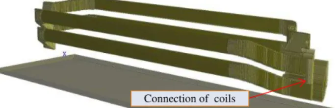
B. Diagnosing of Multiple Discharges in Two Adjacent and Connected Hydro-generator’s Coils Two identical coils discussed in the previous case were electrically interconnected, as illustrated in
Fig. 13. For this case, it was used a computational grid of 864 × 254 × 210 cubic Yee cells with edge
Δ = 2 mm. The sensor location and others characteristics of the simulations are identical to the case
for a single coil. It is noteworthy that, as in the real machine, the inner copper parts of the two coils
were placed in short circuit. Additionally, dielectric layers of both structures were joint, as well as the
outer layers of metal, creating a single structure.
Fig. 13. Two adjacent connected coils.
Fig. 14 shows the obtained results. For this case of two adjacent coils, in about 81% of the
simulations, the results (Fig. 14) enable accurately estimate the positions of the two simultaneous
discharges, even if they occur at different coils. In the remaining cases, the location of the first
discharge was predicted correctly and places near the actual position of the second discharge were
the actual position of the second discharge; in 39.7% of the tests, deviations between 0.5 m and 1 m
were observed; in 11.5% of cases, there are deviations between 1 m and 1.5 m and, in no more than
1.4% of cases the position was estimated with uncertainty of 1.5m to 2m.
(a)
(b)
Fig. 14. Statistical diagnosis for two adjacent coils for several simulation indices: (a) 0 to 20 and (b) 21 to 41.
IV. FINAL REMARKS
A new methodology for localization of partial discharges, based on spectral analysis, was
developed. The FDTD method was used to simulate the electromagnetic process of the problem. We
succeeded to localize multiple partial discharges occurring in a single hydro-generator coil and in two
adjacent interconnected coils. In summary, the technique is based on the determination of frequencies
of resonance of the propagation channels between the position of the transmitter (PD source) and of a
receiver (voltage sensor) inside the hydro-generator’s coil. With this information and by taking into
account the linearity of Maxwell’s equations and of Fourier transform, a probability map of
discharges occurrence as a function of coordinates is obtained. This allows one to define regions
where problems with isolation can exist.
For the case of a single coil, in approximately 90% of the simulations estimates with maximum
discharges positions were predicted with 0.5 m deviation. In the remaining 10% of the simulations,
the position of the first discharge was properly estimated with a few centimeters of deviation from its
exact position and the second discharge was pinpointed within 1.5 m of uncertainty.
Similarly, for two adjacent coils, in about 81% of the simulations it was possible to estimate the
exact location of one of the partial discharges and in 47% of the numerical experiments, the second
discharge position estimation presented 0.5 m or less of deviation.
The obtained simulation results confirm the effectiveness of the localization method proposed in
this paper. Two comments on a practical realization of the method are as follows. Firstly, when there
are many PDs in the investigated system, only the most dangerous PDs with high level of amplitudes
can be tracked and localized. Secondly, in our work, we supposed that the sensors are ideal and do
not introduce any distortion in the PD signals. In the analysis of the obtained real signals, the spectral
characteristics of the used sensors and the electronic processing devices should be taken into account.
Our method, as presented in this paper, is intended to be used for coils extracted from the generator.
The proposed method can be useful for accelerating maintenance (repairing) procedures as long as the
coil is subjected to a laboratory generated 60 Hz signal with sufficient amplitude to produce PDs at
the insulation discontinuity spots.
In a future work, we plan also to investigate the influence of existing noise in real devices on the
proposed methodology and verify the developed method experimentally. It is also planned to employ
(and possibly to adapt) the proposed method to perform localization of other type of discharges, such
as those related to lamination, winding and slotting. It is also intended to develop methodologies for
pinpointing PDs inside the generator during its operation state.
APPENDIX –LABORATORIAL VERIFICATION OF SPECTRAL SIGNATURES IN REAL ROEBEL BAR WITH
INJECTION OF ARTIFICIAL PDSIGNALS
In order to validate our numerical simulator and verify the physical behavior producing the unique
spectral signatures for different propagation channels between each PD occurrence point and each
sensor position, as described in Sections II.B-II.D, laboratorial experiments have been conducted in
this work. We have used a hydro-generator bar extracted from Tucuruí hydroelectric power plant. The
bar used is formed by three layers (inner cooper conductor, the mica insulator and a semiconducting
coating) and has the following dimensions: 2.92 m × 18 mm × 64.3 mm. The measurement setup is
Fig. 15. Setup conceived for obtaining artificial PD spectral signatures.
In order to guarantee full control of excitation positions and waveform of partial discharges at the
points P1 to P6 indicated in Fig.15, a new excitation schema shown by Fig.16 was developed in this
work. Artificial PD signals produced by means of an arbitrary wavefunction generator were injected
into specific points of the Roebel bar. Differently from experiment described in Fig.17 [17], in this
experiment the center conductor of coaxial cable penetrates the insulation, reaching the Roebel bar
inner cooper core, and the cable’s shielding conductor pervades the mica insulation in such way its
lower end is separated from Roebel metallic core by 2 mm. The intention is to experimentally model
localized PDs. Fig. 17 shows the signal injected during experiments (in time and frequency domains).
As illustrated in Fig. 17b, signal energy is distributed in the frequency range from a few Hertz to
approximately 200 MHz.
Two directional couplers [20]-[22] have been manufactured and used as ultrawideband field sensors
[21] (Fig.18). The couplers have been placed in winding slot of the structure, as shown in Fig.15, for
obtaining proper sensing levels. The coupler return loss S11 was measured experimentally and
calculated via FDTD simulation. Observe that S11 is smaller than -15 dB from ~100 Hz to 1.80 GHz
(Fig.19). A good agreement between the measured and simulated return loss is observed.
Mathematically, the return loss is given by
20log10
,11 f f
S (3)
in which
. 0 0 z Z z Z f (4)In (3) and (4),
f
is the reflection coefficient obtained at the SMA connector port, which can beseen in Fig. 18(b), Z is the impedance of the coupler and z0 = 50 Ω is the impedance of the instrument
(oscilloscope or spectrum analyzer) connected to the coupler. Thus, S11 is a measure of impedance
matching between the coupler and the measuring instrumentation as a function of the frequency f.
Fig. 16. The injection of artificial PD signal schema (illustrated at P1).
Fig. 17. Signal injected during experiments: (a) time domain waveform and (b) frequency domain spectrum.
Figure 18. Directional coupler: a) bottom view, b) top view.
Center Conductor
Shielding conductor
Roebel bar inner cooper conductor
Coaxial Cable
Mica Insulator Semiconducting
Coating
Time (ns)
(a)
V
ol
ta
ge
(V
)
S
pe
ct
rum
of
V
ol
ta
ge
Frequency (MHz)
(b)
15.0
0 100 200 300 400 500 600 700 800
0 7.50 22.5
Substrate
R = 50 Ω Microstrip line
Central conductor weld
of SMA connector SMA Connector
Ground Plane(Copper)
Fig. 19.Simulated (FDTD) and measured return loss of microstrip directional coupler.
Fig. 20 shows voltage spectral responses obtained by both couplers in Fig.15 for pulse injection
points P1, P3 and P5. It is of fundamental importance to observe that as the injection point is changed,
resonance frequencies are gradually shifted. As long as the bar in Fig.15 is not prismatic or
symmetrical (it is formed by several quasi-prismatic pieces), certain frequencies of maxima and
minima emerge due to the proximity (or distance) of the source to specific curves of the structure.
Notice that a quasi-prismatic piece of the bar (ℓ1- ℓ5 in Fig.15) produce specific resonances due to its
particular dimensions.
In order to validate the local PD excitation schema developed in this work, we numerically
reproduce the experiment depicted by Fig. 21. The bar of Fig. 15 was excited at point P2 and a
directional coupler was placed 30 cm from the excitation location. The developed numerical model is
shown by Fig. 22. Comparison of numerical and experimental voltage waveforms is shown by Fig.23,
in which it is seen very good agreement between numerical and experimental voltage spectra. Small
difference between numerical and experimental results is attributed to staircase effect in FDTD grid in
curved parts of the structure. Thus, all experimental results are in agreement with theoretical and
numerical investigations in this work. Measurements show that resonances are strongly dependent on
geometric parameters of the bar and on discharge and sensor positions, producing predictable spectral
patterns. This confirmation validates the methodology proposed in this work.
0 200 400 600 800 1000 1200 1400 1600 1800 2000
-45 -40 -35 -30 -25 -20 -15 -10
Frequência (MHz)
S
11
(d
B
)
Simulado Medido
Frequency (MHz)
R
et
u
rn
L
o
ss
(d
B
)
(a)
(b)
Fig. 20. Spectra of experimental voltage signals received by directional couplers for artificial PD injection at points P1, P3, and P5: (a) signals registered using coupler 1 and (b) signals recorded employing coupler 2.
Fig. 21. Injection point P2 and directional coupler over the bar in experimental setup.
Fig. 22. FDTD model of the hydro-generator bar and directional coupler: numerical representation of experimental setup.
Injection point P2 Directional coupler
Injection point P2
Directional coupler
Fig. 23. Comparison of numerical and experimental voltage waveforms obtained with the directional coupler placed over the hydro-generator bar.
ACKNOWLEDGMENTS
Authors would like to thank Eletronorte for financial and laboratorial support. We also would like
to thank Prof. Gervásio Cavalcante and Miércio Alcântara for allowing us to use UHF measurement
equipment.
REFERENCES
[1] D. R. Bertenshaw and A. C. Smith, "Field correlation between electromagnetic and high flux stator core tests," 6th IET
International Conference on Power Electronics, Machines and Drives (PEMD), pp. 1-6, 2012.
[2] J. C. Akiror, A. Merkhouf, C. Hudon and P. Pillay, “Consideration of design and operation on rotational flux density
distributions in hydro-generator stators”, International Conference on Electrical Machines (ICEM), pp. 93-99, 2014.
[3] W. Wang, C. R. Li, W. Li, L. Liu, Z. Wang, and L. Ding, “Pattern recognition of single and composite partial discharge
on generator stators”, Annual Report Conference on Electrical Insulation and Dielectric Phenomena, pp. 335-339, 2001.
[4] D. Wenzel, H. Borsi and E. Gockenbach. “Partial discharge recognition and localization on transformers via fuzzy
logic”, Conference Record of the IEEE International Symposium on Electrical Insulation, pp. 233-236, 1994.
[5] S. Birlasekaran, “Identification of the type of partial discharges in an operating 16kV/250 MVA generator”, Conference
on Electrical Insulation and Dielectric Phenomena, Annual Report. pp. 559-562, 2003.
[6] A. Kheirmand, M. Leijon, and S. M. Gubanski, “Advances in online monitoring and localization of partial discharges in
large rotating machines”, IEEE Transactions on Energy Conversion, 19 (1), pp.53-59, March 2004.
[7] R. Bozzo, C. Gemme, F. Guastavino, and G. Guerra, “Localization of partial discharge sites on power generator bars by
means of ultrasonic measurements”, IEEE lnstumentation and Measurement Technology Conference, pp. 658-663,
May 1997.
[8] H. R. Mirzaei, A. Akbari., E. Gockenbach, M. Zanjani, and K. Miralikhani, “A novel method for ultra-high-frequency
partial discharge localization in power transformers using the particle swarm optimization algorithm”, IEEE Electrical
Insulation Magazine, 29 (2), pp. 26-39, 2013.
[9] S. Biswas, C. Koley, B. Chatterjee, and S. Chakravorti, “A methodology for identification and localization of partial
discharge sources using optical sensors”, IEEE Transactions on Dielectrics and Electrical Insulation, 19 (1), pp.18-28,
2012.
Simulation Experiment
Frequency (Hz)
No
rmali
zed
Spe
[10] S. M. Hoek, A. Kraetge, O. Kessler, and U. Broniecki, “Time-based partial discharge localization in power transformers
by combining acoustic and different electrical methods”, International Conference on Condition Monitoring and
Diagnosis (CMD), pp. 289-292, 2012.
[11] Institute of Electrical and Electronics Engineers, “IEEE Trial-Use Guide to the Measurement of Partial Discharges in
Rotating Machinery”, IEEE Std. 1434 , 2000.
[12] Institute of Electrical and Electronics Engineers, “Guide to Measurement of Partial Discharge in Rotating Machinery”,
IEEE Std 1434, 2000.
[13] F. T. Ulaby, Electromagnetics for Engineers, Prentice Hall, 2005.
[14] M. N. O. Sadiku, Elements of Electromagnetics, Oxford Series in Electrical and Computer Engineering, 2000.
[15] Siemens, “Electrical datasheet: U.H.E Coaracy Nunes–Gerador de Salient Poles 1DH7139-3WF24-Z”, 1997.
[16] R. M. S. de Oliveira and C. Sobrinho, “Computational environment for simulating lightning strokes in a power
substation by Finite-Difference Time-Domain Method”, IEEE Transactions on Electromagnetic Compatibility, 51 (4),
pp.995-1000, Nov. 2009.
[17] O. Lesaint, T. Lebey, S. Dinculescu, H. Debruyne, and A. Petit, “Propagation of fast PD signals within stator bars
performance and limitations of a high frequency monitoring system”, Proceedings of the 7th International Conference
on Properties and Applications of Dielectric Materials, pp. 1112-1115, 2003.
[18] Z. Liu, T. R. Blackburn, B. T. Phumg, and R. E. James, “Detection of partial discharge in solid and liquid insulation
with an electric field sensor”, Proceedings of International Symposium on Electrical Insulating Materials, in
conjunction with Asian International Conference on Dielectrics and Electrical Insulation and the 30th Symposium on
Electrical Insulating Materials, pp. 661-664, 1998.
[19] A. Taflove, and S. Hagness, Computational Electrodynamics: The Finite-Difference Time-Domain Method, Artech
House, 2005.
[20] S. R. Campbell, G. C. Stone, and H. G. Sedding, “Application of pulse width analysis to partial discharge detection”,
IEEE International Symposium on Electrical Insulation, pp. 345-348, 1992.
[21] G. C. Stone, H. G. Sedding, N. Fujimoto, and J. M. Braun, “Practical Implementation of Ultrawideband Partial
Discharge Detectors”, IEEE Transactions on Electrical Insulation, 27 (1), pp. 70-81, 1992.
[22] B. M. Oliver, “Directional Electromagnetic Couplers”, Proceedings of the Institute of Radio Engineers, pp. 1686-1694,
![Fig. 6. (a) 3D view of the hydro-generator coil in SolidWorks ® ; (b) inner structure of the model represented by the SAGS [16] FDTD simulator](https://thumb-eu.123doks.com/thumbv2/123dok_br/18888115.424326/8.892.214.707.326.506/hydro-generator-solidworks-inner-structure-model-represented-simulator.webp)