NON-LINEAR TESTS OF WEAKLY EFFICIENT MARKETS: EVI- DENCE FROM PORTUGAL ()

Esruoos DE EcoNOMIA, vaL. XIX, N.' 2, PRIMAVERA-1999

NON-LINEAR TESTS OF WEAKLY EFFICIENT MARKETS:

EVI-DENCE FROM PORTUGAL

(*)

Antonio Afonso (**)

Joiio Teixeira

(***)

1 - Introduction

No matter how we try to make it so, the world is not orderly: nature is not orderly, nor are the human creations called institutions. Economies and the capital markets

are particularly lacking in orderliness. The capital markets are our own creation; yet we

do not understand how they work. 1 ... ] current capital market theory is based on a linear view of the society. 1 ... ] However, people, and nature in general are nonlinear.

Chaos and Order in the Capital Markets (1996), EaGAR PETERs

An efficient financial market can be described as one for which no deterministic pattern can be detected. Market efficiency implies the absence of pure arbitrage opportunities and denies the profitability by the use of historical data. Efficiency validation is sometimes reduced to test whether the returns generating process of a certain asset is deterministic (evidence against market efficiency) or stochastic (evidence for market efficiency).

Most papers concerning the issue of financial market efficiency used to test the weak form efficiency hypothesis by performing runs tests or autocorrelations

tests. Usually we accept the existence of linear independence for a series P

(for instance stock prices) when it is generated by a (logarithmic) random walk model, given by:

(1)

where

u

₁ is an independent and identically distributed (iid) random variable with zero mean and finite variance (often called «White noise») and C is a constant drift. Evidence that logP follows a random walk is a sign to accept the weak form efficiency hypothesis then returns, the log changes in prices, are unpredictable

C).

(*) The authors are grateful for helpful comments from Miguel St. Aubyn, and participants in

conferences at ISEG, namely in the «II Conference or.t Complexity in Economics» and in the "1st ClEF Workshop on Financial Economics». The usual disclaimer applies.

(**) lnstituto Superior de Economia e Gestao, Universidade Tecnica de Lisboa and lnstituto de Gestao do Credito Publico. Corresponding author (e-mail: [email protected]).

EsTUDOS DE ECONOMIA, VOL. XIX, N.0 _{2, PRIMAVERA 1999}

If the logarithmic price process follows a random walk then the present and past returns R, where:

(2)

are not associated with future returns and hence they have no predictability for

future values of

R.

Therefore,

R;s

independence implies the existence of an

efficient market and univariate time series methods won't succeed in capturing any returns process patterns.

However, even if there is no linear dependence that does not rule out non-linear dependence. In fact, non-non-linear dependence may exist in a series even if we have already concluded for the lack of linear dependence. If present, non-linear dependence would contradict the random walk model and the financial market weak form efficiency hypothesis. Checking if autocorrelation coefficients are not statistically different from zero is not enough. It is therefore necessary to test for the non-linearity of returns.

Brock, Hsieh and LeBaron (1991) mention several tests for non-linearity (2).

In our attempt to validate the weak form efficiency hypothesis, we are going to use the Engle test, the Tsay test, the Hinich bispectrum test, the Lyapunov exponent test and the BDS statistic

(3).

In the next section we introduce the data and describe the series main statistical feature_s. Section three offers a summary description of the non-linearity tests used in the paper, section four presents the empirical results and section five concludes.

2 - Preliminary data exploration

The assumption often assumed, in finance theory, that prices move randomly and that returns are id~ntically distributed following a normal distribution is very handy even if quite unrealistic (4). The main reason for that assumption seems to be related to the fact that the normal distribution is characterised by only two parameters: its mean and its standard deviation. Actually, there is a large consensus among researchers on several stylised facts about the statistical properties of financial time series returns. For instance it is a well-known fact that returns distributions are not normal but rather thick-tailed (leptokurtic). Taylor (1986) presents a review of this topic.

(2) Other useful tests for detecting the presence of non-linearity are used by Lee, White and Granger (1993) and Brooks (1996).

(3) AI-Lougahni and Chappell (1996) call this a new test in opposition to runs tests and autocorrelation tests.

Esruoos DE EcoNOMIA, voL. x1x, N.0 _{2, PRIMAVERA 1999}

In this study we analyse three financial time series: the BVL (Bolsa de Valores de Lisboa) General Index, the PSI20 (Portuguese Stock Index 20) Index and the BVL30 Index. These are composite stock market indexes that reflect the aggregate movements of the Portuguese stock market. Since the Portuguese financial market is a very thin one, individual stock prices don't seem to be a good choice.

The available data tor those indexes allow us to use more than 1700 daily observations tor BVL and around 1200 observations tor the PSI20 and BVL30 series (5). The accurate samples and its main statistical features are described bellow on Table 1 and the three series are plotted on figures 1, 2, and 3 (all figures are presented on the annex).

TABLE 1

Descriptive statistics for BVLG, PSI20 and BVL30

Sample

Index N Mean S.d. Minimum Maximum

From To

BVLG ... 1990-01-10 1998-01-06 1793 909.17 333.88 537.20 2014.53

PSI20 ... 1993-01-04 1998-01-06 1239 4764.17 1405.29 2917.56 9294.05

BVL30 ... 1993-01-05 1998-01-06 1238 1922.99 672.32 980.14 3992.42

Note. - N is the number of observations in sample.

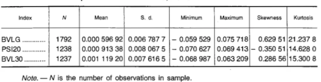
Table 2 gives a selection of descriptive statistics tor the daily log returns. The log returns are also represented on figures 4, 5, and 6. All three series returns show strong departure from normality, as the coefficients of skewness and kurtosis are statistically different from those of a normal distribution (6_{). All}

three series are leptokurtic and have asymmetric tails: PSI20 is skewed to the lett and both BVLG and BVL30 are skewed to the right.

TABLE 2

Descriptive statistics for BVLG, PSI20 and BVL30 returns

Index N Mean S.d. Minimum Maximum Skewness Kurtosis

BVLG ... 1792 0.000 596 92 0.006 787 7 - 0.059 529 0.075 718 0.629 51 21.237 8

PSI20 ... 1238 0.000 913 38 0.008 067 5 - 0.070 627 0.069 413 - 0.350 51 14.628 0

BVL30 ... 1237 0.001 119 20 0.007 616 5 - 0.068 987 0.063 209 0.286 56 15.300 8

Note. - N is the number of observations in sample.

(5) The reader must be aware that until November 1997 Portuguese capital markets belonged

to the so-called emerging markets category. Since December 2, 1997, the Portuguese Stock Exchange was included in the Morgan Stanley Capital Index for developed markets.

EsTUDOS DE EcoNOMIA, VOL. XIX, N.0 _{2, PRIMAVERA 1999}

3 - Non-linear tests

A brief theoretical presentation of the non-linear tests is given in this sec-tion. The first two tests presented in this section are intended to test for neglected non-linearity and will be applied to the residuals of an AR(p) model. The number of lags was selected using the Schwarz Bayesian Information Criterion (SBIC).

3.1 - Engle's test

Autorregressive conditional heteroescedasticity (ARCH) models were developed by Engle (1982) who also proposed a test that explicitly examines for non-linearity in the second moment. In its simplest form an ARCH (p) process can be written formally as:

yl

=

{31 + {32X21 + .. · + f3,}(kl + El

El- N(O,CJI)

d-

=

ao + a1t.f-1+ a2~-2+ ... + aPt.f-p

(3)

(4)

(5)

The null hypothesis of no autocorrelation in the error variance is

H0 : a₁

=

02

= ... =

aP

=

0, which if accepted would lead us to deny the existence of an ARCH (p) model. The procedure to test that hypothesis is as follows:

1) Regress _Y1 linearly on _X1 (if the information set, _X1, is restricted to

the past observations of Y₁ then we simply estimate an AR (p)

process) and save the estimated residuals ~

₁

;

2) Regress the squares of the estimated standard residuals on an intercept and p lagged values of

fJ

as:

(6)

and save the estimated residuals;

3) Calculate the F{2 from the second regression and test the null

hypothesis using the

nf/2

statistic that follows a X2(p) distribution under the null of no ARCH dependence.

3.2 - Tsay's test

While the Engle test examines evidence for non-linearity in the variance the Tsay test checks for non-linearity on the mean(). The procedure to compute the test proposed by Tsay (1986) is as follows:

1) Regress Y₁ linearly on X₁ (in practice we estimate an AR model if the information set, X₁, is restricted to the past observations of Y

1)

and keep the estimated residuals ~~;

EsTUDOS DE EcoNOMIA, VOL. XIX, N.0 _{2, PRIMAVERA 1999}

2} For each observation of Y₁ build the vector Z₁ of the cross products of past observations in other words, Y₁_;Y₁_j fori, j

=

1, ... , p where

i~j. For example if p

=

2 then Z₁

=

[~_ ₁,

y;

_

₁ Y₁__2, ~_

2

]T (notice that

our vector Z₁ has p(p + 1 }/2 elements);

3} Regress the vector Z₁ on the explanatory variables and save the estimated residuals ry₁;

4) Regress the estimated residuals ~~ on

f1r

(7)

1\

and save the estimated residuals ~P

5) Calculate the Tsay test statistic:

(8)

where m

=

p(p + 1 }/2 and test the null hypothesis:

Tsay {1986} showed that the statistic (8) has an F(m, n-p-m-1} distribution under the null hypothesis and is sensitive to departures from linearity in the mean.

3.3 - Hinich bispectrum test

The Hinich bispectrum test is used to estimate the bispectrum of a stationary time series and provides a direct test for non-linearity and also a direct test for Gaussianity (8). If the process generating the data (in our case the rates of return) is linear then the skewness of the bispectrum will be constant. If the test rejects constant skewness then a non-linear process is implied.

Linearity and Gaussianity can be tested using a sample estimator of the skewness function

r

(w₁,w₂) with:

(9)

Esruoos DE EcoNOMIA, voL. XIX, N.' 2, PRIMAVERA 1999

where Sxx(w) is the spectrum of x(~ at frequency

w.

The bispectrum at frequency pairs (w₁, w₂) is defined as:

8 (W W )

= "" ""

c

(rs)el-i27t(W1f+ W2S)]

XXX 1 ' 2 .£... .£... XXX ' (10)

r=-oo S=-oo

in the principal domain given by Q = {(w₁,w₂): 0 < w₁ < 0.5,

w

₂ < w₁, 2w₁ +

w

₂ < 1}.

The null of the Hinich <<linearity» test is actually given by:

H₀: flat skewness function, absence of third order non-linear

depen-dence;

H_{1 :} non-linear dependence, absence of efficiency;

and H₀ is rejected if the standard normal test statistic Z is large, over. 2 or 3. When the null is Gaussianity the related test statistic is denoted by H and is also a standard normal random variate under the null.

3.4 - Lyapunov exponent

Lyapunov exponents measure the exponential rate at which two nearby orbits are moving apart. They provide an estimate of sensitive dependence on initial conditions, a defining feature of chaos. It basically means that if we allow for small changes in the state of a system it will grow at an exponential rate. Consider two points,

x

₀ and

x

₀ + £, apart from each other by only the infinitesimal difference e and apply a map function to each of the two points n times. (9_{) The difference between the results is given by:}

d = enil(Xo) £

n (11)

and after solving for the convergence (or divergence) rate A we have the Lyapu-nov exponent:

A= lim

.2_

log

1.:±_1

n->~ n £ (12)

If a system has at least one positive Lyapunov exponent then the system is chaotic and trajectories, which start at two similar states, will diverge exponentially. The larger the dominant positive exponent the more chaotic the system and the shorter the time span of system predictability. A positive Lyapunov exponent is therefore viewed as «an operational definition of chaotic behavior»

(1°).

In an earlier paper Wolf, Swift and Vastano (1985) estimated the Lyapunov exponent by averaging the observed orbits divergence rates. Some authors

Esruoos DE EcoNOMIA, VOL. XIX, N.0 _{2, PRIMAVERA 1999}

however argue that this method is less reasonable when we are dealing with noisy systems. Therefore McCaffrey, Ellner, Gallant and Nychka (1992) and Nychka, Ellner, McCaffrey and Gallant (1992) use an alternative approach based

on Jacobian methods in order to avoid upward bias when estimating Lyapunov

exponents

C

1

).

3.5-BDS test

(1

2₎

The BDS test can only be used to produce indirect evidence about non-linearity because the sampling distribution of the test statistic is not known. This statistic is useful to test for patterns that occur more (or less) frequently than would be expected in independent data. The BDS test can be used to test for the remaining non-linear dependence in the residuals of an ARIMA process. The null hypothesis may be formulated as:

H_{0 :} pure whiteness, independent data, data generated by an iid

stochastic process, efficiency;

H1: non-linear dependence, absence of efficiency;

and when the BDS test statistic is large (which means larger than 2 or perhaps 3), H₀ is rejected.

Before looking at our results we briefly present the BDS test of indepen-dence and identical distribution or the so-called BDS test for non-linearity.

The Brock-Dechert-Scheinkman (BDS) statistic is a non-parametric test to assess the null hypothesis that a univariate series {x₁, f= 1 , ... ,n} is independently

and identically distributed against an unspecified alternative. This test is performed by examining the underlying probability structure of {x₁} in order to search for

any kind of dependence. Often referred as a non-linear test, the BDS statistic can be used to detect any deviation from independence even if due to the presence of non-linear dependence in the data.

Let us define the correlation integral, given by equation (13), as a measure of the fraction of pairs of points (Xf,~) in the series that are within a distance of £ (metric bound) from each other:

N-1 N

c~(c:)=

N(N~1)

L

L

1(xr:x;> (13)

I= 1 S=i+ 1

(11 ) S. Ellner, D. W. Nychka and A. R. Gallant developed the LENNS (Lyapunov Exponent of Noisy Nonlinear Systems) software, a program that also estimates the dominant Lyapunov exponent and tests for chaos. Unfortunately we were not able to get an executable version of this software.

ESTUDOS DE EcoNOMIA, VOL. XIX, N.0 _{2, PRIMAVERA 1999}

with:

l(a,b)=

{1

if

lla--:-bii::;E

0 otherw1se

where

II. II

is the supremum norm (L~

=

max {

I

a

I } )

and

N=

n-

m+ 1;

n-

number of observations; and

m-embedding dimension.

(14)

In the literature,

xm

is commonly referred to as the m-history and can

generally be written as

xr=

(xl'x₁+_{1, ...} x₁+m-_1). For instance, with m= 2, the first

3 histories will be: (xl'x₁+_1), (x₁+₁,x₁+₂₎ and (x₁+₂,x₁+₃). Observe that since the first and third history do not have any repeated element, they are said to be non-overlapping histories.

If the data is generated by a strictly stationary stochastic process, which is absolutely regular, then equation (13) can also be written as:

(15)

and Brock, Dechert, Sheinkman and LeBaron (1991) show that if {x₁} is iid then

We have Cm (E)= C_{1 (E)m.}

The BDS statistic is then given by:

(16)

where W~(c:) converges in distribution to a standard normal, N(O, 1 ), as n approa-ches infinity

(1

3). Brock, Hsieh and LeBaron (1991) show that the normal distri-bution was found to be, asymptotically, a good approximation for the distridistri-bution of the BDS statistic when there are more than 500 observations.

One should be aware that the BDS statistic depends, to a great extent, on the choice of values for e and

m.

With large (small) e the spatial correlation between the data points will tend to be high (low). The greater is the embedding dimension the smaller will be the number of non-overlapping histories and, as a consequence, the points defined by the embedded vectors will become <<closer»

Esruoos DE EcoNOMIA, VOL. XIX, N.0 _{2, PRIMAVERA 1999}

and the value of the BDS statistic will tend to be higher. For a large absolute value of the test statistic we reject the null hypothesis of iid (randomness) since this provides evidence that the data are non-linear.

4 -Empirical results

Non-linear dependence may not be absent from the stock exchange returns. In order to validate that hypothesis we now proceed our work by testing for neglected non-linearity.

Engle and Tsay test results

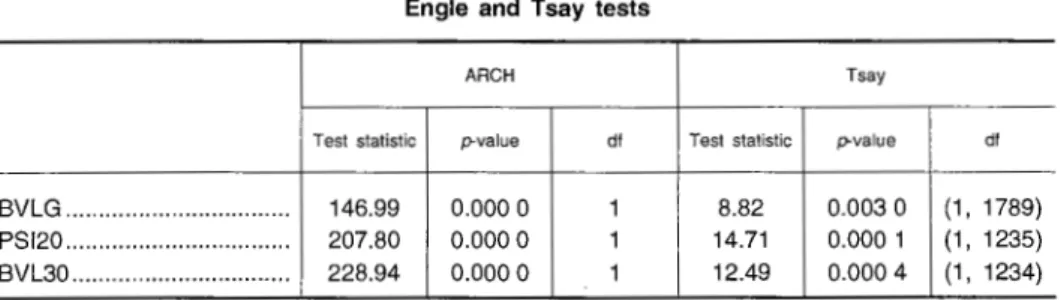
After selecting an AR(1 ), for the log returns of the three stock exchange indexes (using the SBIC), we applied the two tests to the residuals of the AR(1) model. The results are reported in table 3 and allow us to reject the null hypothesis in both cases. This means that we can neither conclude for the absence of an ARCH (1) model using the Engle test (there may be non-linearity in the variance) or for the lack of non-linearity on the mean using the Tsay test (14_).

TABLE 3

Engle and Tsay tests

ARCH Tsay

Test statistic p-value df Test statistic p-value df

BVLG ... 146.99 0.000 0 1 8.82 0.003 0 (1' 1789)

PSI20 ... 207.80 0.000 0 1 14.71 0.000 1 (1, 1235)

BVL30 ... 228.94 0.000 0 1 12.49 0.000 4 (1, 1234)

Note. - df - degrees of freedom.

Hinich test Results

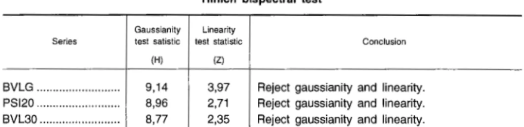
Without prewhitening and using the first differences of the natural logarithms of our stock exchange indexes we performed the Hinich bispectrum test. We did not use previously any linear filtering of the data since Ashley, Patterson and Hinich (1986) proved that the Hinich test is invariant to linear filtering. If the original series were non-linear then the non-linearity would pass through the linear filter to the residuals.

Esruoos DE EcoNOMIA, VOL. XIX, N.0 _{2, PRIMAVERA 1999}

The evidence from table 4, rejection of linearity with the Hinich test, sup-plies support for the conclusion on non-linearity in Portuguese stock indexes returns and therefore for the absence of weak form efficiency

(1

5).

TABLE 4

Hinich bispectral test

Gaussianity Linearity

Series test satistic test statistic Conclusion

(H) (Z)

BVLG ... 9,14 3,97 Reject gaussianity and linearity. PS120 ... 8,96 2,71 Reject gaussianity and linearity. BVL30 ... 8,77 2,35 Reject gaussianity and linearity.

Note. -the tests are one sided and the null hypothesis is rejected in both cases if the test statistic exceeds 2 or 3. As suggested by Hinich (1982) the bispectral smoothing parameter was set to approximately the square root of the number of observations.

However, even if we did not reject the null of linearity, one should be aware, as reminded by, Barnett, Gallant, Hinich, Jungeiles and Jensen (1997), that «acceptance of the null of linearity [ ... ] provides only weak support for the linearity, since the [Hinich] test, as currently constructed, actually tests the broader null of absence of third order nonlinear dependence»

(1

6 ).

Estimates of Lyapunov exponents

Table 5 presents estimates of the maximum Lyapunov exponents, of the daily log returns series, using the estimation method of Wolf et a/. (1985)

(1

7).

We computed the Lyapunov Exponents with embedding dimensions up to five which, considering the available data, is already more than the value suggested by Wolf (1991).

(15) Our calculations were obtained with software developed by D. M. Patterson (Bispectrum Estimation Program, Version 5.11, September 1992).

(16) The interesting paper of Barnett, Gallant et a/. (1997) concerning non-linearity and tests for chaos may be found in http://wuecon.wustl.edu/-barnett!Papers.html.

(17_{) We computed the Lyapunov exponents with a software developed and distributed by A.}

Wolf (programs BASGEN and FET, 1991). These programs may be obtained from A. Wolf's Web site, http://www.users.interport.net!-wolf/, in a self-decompressing executable file. Wolf (1991) provides valuable indications on how to use those programs.

Esruoos DE EcoNOMtA, voL. xtx, N.' 2, PRIMAVERA 1999 TABLE 5

Lyapunov exponents for log returns

Ndim

1 ... . 2 ... . 3 ... . 4 ... . 5 ... .

BVLG

0.0144 0.0155 0.0204 0.0291 0.0136

max A

PS120

0.0216 0.0130 0.0135 0.0168 0.0099

BVL30

0.0120 0.0282 0.0205 0.0144 0.0167

Note. - max A.-maximum estimated value of Lyapunov exponent; ndim - embedding di-mension.

The results, all I are positive, seem to point to the above stated operational definition of chaos: trajectories that start at two almost identical state vectors diverge exponentially as time passes, allowing us to accept chaos for our three financial time series.

If chaos exist one implication is that profitable non-linearity based trading rules exist at least in the short-run. The problem would then be to find out the generating mechanism in order to take advantage of the financial markets inefficiencies.

The BDS test

The BDS test will be applied to the residuals of a fitted linear model, in our case an ARIMA model, which we presumed has extracted as much linear structure as possible from the data.

Using the Box-Jenkins methodology we tried to adjust an ARIMA (autore-gressive integrating moving average) process for each of our chosen stock

exchange indexes log returns. Briefly, we fitted an ARIMA (p, d, q) model to

our time series, where p denotes the number of autoregressive terms, d the

number of times the time series has to be differenced before it becomes stationary, and q is the number of moving average terms

(1

8

).

Visual inspection may be used (see figures 4, 5 and 6 on the annex) to assess, as a preliminary step, whether the series are stationary. In fact, the Box-Jenkins methodology applies only to stationary data series, which means that the time series has a mean and a variance essentially constant through time. Together with the analysis of the correlograms of the autocorrelation and partial

(18 ) We did not restrict our linear specifications to an autoregressive form, solution used for instance by Brooks (1996).

Eswoos DE EcoNOMIA, VOL. XIX, N.0 _{2, PRIMAVERA 1999}

autocorrelation functions we tentatively identified an ARIMA (0, 1, 3) model for the returns of the three original time series. Using the lag operator L, that is:

LXt=Xt-1

our ARIMA models assumed the form:

(17)

(18)

where Y is the first difference of the natural logarithm of the original time series, 8₁, 8₂ and 8₃ are the moving average coefficients and the random shock

u

₁ is

assumed to be an iid random variable with a mean of zero and a constant variance.

Table 6 presents the main results of the fitted models, which satisfy the stationarity and invertibility conditions (19). The residuals of the ARIMA models will now be used to perform the BDS test.

TABLE 6

ARIMA models for Stock Exchange Indexes daily returns

Index Model e, e2 e,

BVLG ARIMA(O, 1 ,3) ... Coefficient ... 0.802 075 0.137 213 0.050 019

T-Statistic ... 33.97 4.55 2.12

PSI20 ARIMA(O, 1 ,3) ... Coefficient ... 0.791 847 0.133191 0.067 637

T -Statistic ... 27.91 3.69 2.38

BVL30 ARIMA(0,1,3) ... Coefficient ... 0.799 907 0.106 930 0.08 518

T -Statistic ... 23.18 2.94 2.99

Note. - ei is the parameter for an MA at lag i.

To compute the BDS statistic Brock, Hsieh and LeBaron (1991) recommend using e between one-half to two times the standard deviation of the raw data (0,5 cr :::;; £:::;; 2 cr) while suggesting that m = 2. For samples with less than 500 observations m should be set less or equal to 5.

Table 7 presents the results of the BDS test for the ARIMA residuals of log returns

(2°).

It can be seen that the null hypothesis of R₁ being iid is rejected, at the 5 per cent level, for all indexes.

(19) These models are always stationary since they have no autoregressive coefficients. The invertibility conditions require that for I ei I <all i.

(20 ) Our BDS statistics were obtained with software developed by William Dechert (BDS

STATS, version 8.20). The interested reader may try to get the BDS software either from http:// www.ssc.wisc.edu/-lebaron/software/index.html or from the alternative web site gopher:// gopher.ssc.wisc.edu/00/econgopher/software/bds/dos.

ESTUDOS DE EcDNOMIA, VOL. XIX, N.0 _{2, PRIMAVERA 1999}

Table 7

BDS statistics - Residuals from the ARIMA to log returns

e

Index m

0,5cr

"

1,5cr 2cr

BVLG ... 2 14.719 15.292 13.438 12.064

3 18.322 17.763 14.765 12.933

4 20.876 19.319 15.644 13.424

5 24.284 21.014 16.187 13.527

PSI20 ... 2 12.178 10.729 10.045 10.450

3 15.219 12.513 10.693 10.550

4 18.407 14.128 11.404 10.834

5 22.656 15.792 12.065 10.929

BVL30 ... 2 11.306 10.615 9.765 9.687

3 14.518 12.297 10.268 9.793

4 17.503 13.905 10.076 10.256

5 21.379 15.583 11.735 10.376

Notes. - m- embedding dimension; e- distance between points, measured in terms of number of standard deviations of the raw data; cr- standard deviation. All statistics significant at the 5 per cent level.

In other words, non-linear dependence is not absent from the series returns and we must therefore conclude that the weak form efficiency hypothesis is not validated for all of the Portuguese stock exchange indexes in our data set

(2

1_).

5 - Conclusions

The hypothesis of linearity is rejected by almost all the tests we computed. In fact, the results allow us to reject the null hypothesis of daily returns being iid, non-linear dependence is present on those returns therefore contradicting the random walk model supposition. Since the test results indicate that non-linear structure is present in the data, it is possible that exploitable excess profit opportunities may exist in the Portuguese stock market

(2

2_).

These conclusions are consistent with the results of Omran (1997) from the UK and of de Lima (1995) from the US since those authors argue that non-linear dependence is present in stock returns after the 1987 crash.

Our results seem therefore to challenge the belief that daily rates of return can be viewed as independent random variables. In fact, those returns may be

(21) These conclusions confirm the results from previous work by Afonso and Teixeira (1997) concerning namely stock exchange index_es for several activity sectors.

(22) Obviously, and as Michael Brennan pointed out to us, non-linearity does not imply predictability.

Esruoos DE EcoNOMIA, VOL. XIX, N.0 _{2, PRIMAVERA 1999}

...

(X) (,)

_.

8 8

I'll

8

c.> 01

8

POINTS

§ §

§

§

31-12-92 +--+--r-r--i-...,....-t---t--,_-t---j

§ §

26-05-93 18-10-93 14-03-94 10-08-94 05-01-95 01-06-95 25-10-95 22-03-96 21-08-96

160197

-17-06-97

05-11-97

I I

- --t - - -J - - -r- - - r- - - r- - -t- - - +~

I I I I I

(/) .... 0 (") ;oo;" ~ (")

:r ₀₁

Ill

Gi

:::s

CQ _c

CD _:n

:;· m c. 1\)

~

I

,

(/) i\i 0 01 0 0 01-10-90 28-02-91 30-07-91 19-12-91 19-05-92 12-10-92 09-03-93 02-08-93 27-12-93 Cl 0 co 0 0 POINT _.

_. c.> 0 0 0 0

_. _.

8

Cl ₀

I I I I

_.

~

0

-r--,---~--~---,--,---r--1 I I

I I I

-~--~---~--~---~--~---r--1

20-05-94 -- - -j ~ '~I - - ~ - -~ - - _, - - -~ _, '

-I I I I I I I

17-10-94

13-03-95

08-08-95

---L--~---L--~---L--1 I I I

05-01-96

31-D5-96

I

24-10-96 _{- - -}

~

_{- - -:- - \ - - -i -- - -}

~

_{: :}

-I 24-03-97 21-08-97 ~ 8 (/) 8" (") ;oo;" ~ (") :r Ill :::s CQ CD :;· c. CD )(

I

m < r-G) "TT Gi c :n m _. l> z z m

X _[;(! [§ 0 "' ~

~

0 ~ ~ ?:s ~ ~

·"'

_]?

~

iii

~

~

...

b b b 0 0 0 0

00 _{0 0 0 0 0 0 0}

,j::o C) .;.. N 0 N .;.. C) CXI

02-10-90 31-01-91 05-06-91 01-10-91 29-01-92 27-05-92 22-09-92 21-01-93 19-05-93

I m

<

13-09-93 I I I I r _G)

-n

I

c. C5

11-01-94 I

Dl _c

I I

-<

:Il

10-05-94 I I m

iil

... .;..

07-09-94 c::

I ₃

05-01-95 I Ul

05-05-95 31-08-95 02-01-96 30-04-96 28-08-96 23-12-96 24-04-97 25-08-97 ~ ~

8

0

g

₈

POINT

~

0

w

0 .;.. 0

0

g

04-01-93

-l----t----+----r---+---1----t----w 01 0 0 N 01 0

0

g

27-05-93

191093

-15-03-94 11-08-94 08-01-95 02-06-95 26-10-95 25-03-96 22-08-96 17-01-97 18-06-97 06-11-97

r T , ,

-1 I I I

I

r t ; ;

-!:\1

I§

g

0

"'

~ ~ 0 ~ ~ ?:s _x.

;;,

]\:> C/) ... 0 () ;o; (II >< () ::r

Dl -n :I _C5

Ul

(II c

:i"

:Il m c.

(II w

6 6 6 I I I I I

0 0 0 0 0 0 0 0 0 0 0 0 0

b b _~ b b _~ b b b b ~

2

b _~ b b

00 CJ) N 0 N CJ) 00 00 CJ) 0 N CJ) (X)

05-01-93 04-01-93

25-03-93 I I I I 24-03-93

I

16-06-93 I _15-06-93

I I

03-09-93 I I I I 02-09-93

24-11-93 23-11-93

16-02-94 14-02-94

10-05-94 09-05-94

02-08-94 01-08-94

21-10-94 Ill 20-10-94 "'CI

< (J)

r

15-01-95 w 12-Q1-95 I i\i

0 "T1 0 "T1

G5 I

04-04-95 c. Ill _c 03-04-95 _I I _I c. Ill G5 c

-<

:IJ I

-<

:IJ

29-06-95

..

m 28-06-95 I

..

m _[XI

!2. CJ) !2. 01

18-09-95 c:

..

15-Q9-95 c:

..

§

j j 2

11-12-95 Ul 07-12-95

I Ul

I ~

I I

~

04-03-96 I 01-03-96

I

Q

I

"'

27-05-96 24-05-96

Q

~

I

19-08-96 I 16-08-96 ~

06-11-96 05-11-96 I _J< ?,;

29-01-97

I

;;,

30-01-97 I I I

I I I

_-""

23-04-97 I 22-04-97

I

I I

;r;

I _16-07-97 I ~

17-07-97 I

I ;j\

06-10-97 03-10-97 ~

...

I <0

ESTUDOS DE ECONOMIA, VOL. XIX, N.0 _{2, PRIMAVERA 1999}

REFERENCES

ABHYANKAR, A., COPELAND, L. S., and WONG, W. (1995), «Nonlinear Dynamics in Real-Time

Equity Market Indices: Evidence from the United Kingdom», The Economic Journal, 105 (431), July, 864-880.

AFONSO, A. (1997), «Normality and Efficiency in Portuguese Stock Exchange Indexes», March, Estudos de Economia, XVI-XVII, Fall, 101-106.

AFONSO, A., and TEIXEIRA, J. (1997), <<Efficiency in Portuguese Stock Exchange Indexes: Runs Tests and BDS Statistics••, working paper n.Q 2/97, Department of Economics, Institute Superior de Economia e Gestao, Universidade Tecnica de Lisboa.

AI-LOUGHANI, N., and CHAPPELL, D. (1996), ••On the Validity of the Weak Form Efficient Markets Hypothesis Applied to the London Stock Exchange••, Applied Financial Economics, 7 (2), April, 173-176.

ASHLEY, R. A., PATTERSON, D. M., and HINICH, M. J. (1986), ••A Diagnostic Test for Nonlinear Serial Dependence in Time Series Fitting Errors••, Journal of Time Series Analysis, 7 (3), 165-178.

BARNETT, W. A., GALLANT, A. R., HINICH, M. J., JUNGEILGES, J., KAPLAN, D., and JENSEN, M. J. (1996), ••An Experimental Design to Compare Tests of Nonlinearity and Chaos••, in Nonlinear Dynamics and Economics, eds. William Barnett, Alan Kirman and Mark Salmon, Cambridge, Cambridge U. Press.

BARNETT, W. A., MEDIO, A., and SERLETIS, A. (1997), ••Nonlinear and Complex Dynamics in Economics••, mimeo.

BARNETT, W. A., GALLANT, A. R., HINICH, M. J., JUNGEILGES, J., KAPLAN, D., and JENSEN, M. J. (1997), ••A Single-Blind Controlled Competition Among Tests for Nonlinearity and Chaos••, Journal of Econometrics (forthcoming).

BROCK, W. A., and BAEK, E. G. (1991 ), ••Some Theory of Statistical Inference for Nonlinear Science••, Review of Economic Studies, 58, 697-716.

BROCK, W. A., HSIEH, D. A., and LEBARON, B. (1991), Nonlinear Dynamics, Chaos, and

Instability: Statistical Theory and Economic Evidence, The MIT Press.

BROCK, W. A., DECHERT, W. D., SCHEINKMAN, J. A., and LeBARON, B. (1991), A Test for

Independence Based on the Correlation Dimension, Social Systems Research Institute, University of Wisconsin, March.

BROOKS, C. (1996), «Testing For Non-linearity in Daily Sterling Exchange Rates••, Applied Financial Economics, 6 (4), August, 307-317.

DE LIMA, P. F. (1995), <<Nonlinearities and Nonstationarities in Stock Returns••, Working Papers in Economics, The John Hopkins University, Department of Economics.

ENGLE, R. f. (1982), ••Autoregressive Conditional Heteroskedasticity with Estimates of the Variance of United Kingdom Inflation••, Econometrica, 50 (4), 987-1007.

FAMA, E. (1991), ••Efficient Capital Markets II>•, Journal of Finance, XLVI (5), December, 1575-1617. GUARDA, P., and SALMON, M. (1996), ••Detection of nonlinearity in foreign-exchange data••, in Nonlinear Dynamics and Economics, eds. William Barnett, Alan Kirman and Mark Salmon, Cambridge, Cambridge U. Press.

HINICH, M. J. (1982), ••Testing for Gaussianity and Linearity in a Stationary Time Series••, Journal of Time Series Analysis, 3 (3), 169-176.

HINICH, M. J., and PATTERSON, D. M. (1985), ••Evidence of Nonlinearity in Daily Stock Returns••, Journal of Business and Economic Statistics, 3 (1), 69-77.

HINICH, M. J., and PATTERSON, D. M. (1985), <<Evidence of nonlinearity in the trade-by-trade stock market return generating process••, in W. A. J. Barnet, Geweke, and K. Shell, (eds.), Economic Complexity: Chaos, Sunspots, Bubbles, and Nonlinearity, Cambridge University Press.

Esruoos DE EcoNOMIA, VOL. XIX, N.0 _{2, PRIMAVERA 1999}

LEE, T. H., WHITE, H., and GRANGER, C. (1993), «Testing for Neglected Nonlinearity in Time Series Models: A Comparison of Neural Networks Methods and Alternative Tests", Journal of Econometrics, n.Q 56, 269-290.

MCCAFFREY, D., ELLNER, S., GALLANT, R., and NYCHKA, D. (1992), «Estimating the Lyapunov Exponent of a Chaotic system With Nonparametric Regression", Journal of the American Statistical Association, September, 87 (419), 682-695.

NYCHKA, D., ELLNER, S., McCAFFREY, D., and GALLANT, R. (1992)., «Finding Chaos in Noisy Systems", Journal of the Royal Statistical Society, series B, 54 (2), 399-426.

OMRAN, M. F. (1997), «Nonlinear Dependence and Conditional Heteroscedasticity in Stock Returns: UK Evidence", Applied Economics Letters, 4 (10), 647-650.

SCHEINKMAN, J. A., and LEBARON, B. (1989), «Nonlinear Dynamics and Stock Returns .. , Jour-nal of Business, 62 (3), 311-337.

TAYLOR, S. (1986), Modelling Financial Time Series, John Wiley & Sons.

TEIXEIRA, J. (1997), Previsao Baseada em Modelos Neuronais e de Regressao Dinamica, October, masters dissertation, Faculdade de Ciencias .de Lisboa.

TSAY, R. S. (1986), «Nonlinearity Tests for Time Series", Biometrika, 73 (2), 461-466.

WOLF, A. (1991), «Lyapu-News: documentation for FET, a program that quantifies chaos in time series", mimeo.