Experimental and numerical study of geotechnical problems using the material point method

UNIVERSIDADE DE BRASÍLIA

FACULDADE DE TECNOLOGIA

DEPARTAMENTO DE ENGENHARIA CIVIL E AMBIENTAL

EXPERIMENTAL AND NUMERICAL STUDY OF

GEOTECHNICAL PROBLEMS USING THE MATERIAL

POINT METHOD

MARCELO ALEJANDRO LLANO SERNA

ORIENTADOR: MÁRCIO MUNIZ DE FARIAS, PhD

COORIENTADOR: DORIVAL DE MORAES PEDROSO, PhD

TESE DE DOUTORADO EM GEOTECNIA

PUBLICAÇÃO: G. TD – 121/16

UNIVERSIDADE DE BRASÍLIA

FACULDADE DE TECNOLOGIA

DEPARTAMENTO DE ENGENHARIA CIVIL E AMBIENTAL

EXPERIMENTAL AND NUMERICAL STUDY OF

GEOTECHNICAL PROBLEMS USING THE MATERIAL

POINT METHOD

MARCELO ALEJANDRO LLANO SERNA

TESE DE DOUTORADO SUBMETIDA AO DEPARTAMENTO DE ENGENHARIA CIVIL DA UNIVERSIDADE DE BRASÍLIA COMO PARTE DOS REQUISITOS NECESSARIOS PARA OBTENÇÃO DO GRAU DE DOUTOR.

APROVADA POR:

MÁRCIO MUNIZ DE FARIAS, Ph.D. (UnB) (ORIENTADOR)

DORIVAL DE MORAES PEDROSO, Ph.D. (UQ) (COORIENTADOR)

MARCIO DE SOUZA SOARES DE ALMEIDA, Ph.D. (COPPE-UFRJ) (EXAMINADOR EXTERNO)

RAUL DARIO DURAND FARFAN, D.Sc. (PECC/UnB) (EXAMINADOR EXTERNO)

MANOEL PORFÍRIO CORDÃO NETO, D.Sc. (UnB) (EXAMINADOR INTERNO)

HERNÁN EDUARDO MARTINEZ CARVAJAL, D.Sc. (UnB) (EXAMINADOR INTERNO)

FICHA CATALOGRÁFICA

LLANO-SERNA, MARCELO ALEJANDRO

Experimental and Numerical Study of Geotechnical Problems Using the Material Point Method

[Distrito Federal] 2012

xv, 89 p; 297 mm (ENC/FT/UnB, Doutor, Geotecnia, 2016) Tese de Doutorado – Universidade de Brasília.

Faculdade de Tecnologia, Departamento de Engenharia Civil e Ambiental 1. Grandes deformações 2. Método do Ponto Material

3. Escorregamentos 4. Cone de penetração

I. ENC/FT/UnB II. Titulo (Série)

REFERÊNCIA BIBLIOGRÁFICA

LLANO-SERNA, M. A. (2016). Experimental and Numerical Study of Geotechnical Problems Using the Material Point Method. Tese de Doutorado, Publicação G.TD-121/16, Departamento de Engenharia Civil, Universidade de Brasília, Brasília, DF, 89 p.

CESSÃO DE DIREITOS

NOME DO AUTOR: Marcelo Alejandro Llano Serna

TÍTULO DA TESE DE DOUTORADO: Experimental and Numerical Study of Geotechnical Problems Using the Material Point Method.

GRAU / ANO: Doutor / 2016.

É concedida à Universidade de Brasília a permissão para reproduzir cópias desta tese de doutorado e para emprestar ou vender tais cópias somente para propósitos acadêmicos e científicos. O autor reserva outros direitos de publicação e nenhuma copia para esta dissertação de mestrado pode ser reproduzida sem a autorização por escrito do autor.

_____________________________________ Marcelo Alejandro Llano Serna

30 O‘keefe St.

CEP:4102 – Queensland – Australia e-mail: unalmallano@gmail.com

AGRADECIMENTOS

Ao Professor Márcio, pela confiança e ideias durante o desenvolvimento da pesquisa.

Ao Professor Dorival na Universidade de Queensland pelo apoio durante à visita na Austrália.

Aos meus amigos e colegas.

À Coordenação de Aperfeiçoamento de Pessoal de Nível Superior (CAPES) pelo apoio financeiro, sem o qual esta pesquisa não seria possível.

A todas as pessoas que de uma ou outra forma participaram deste processo. Obrigado.

RESUMO

O objetivo deste trabalho é investigar os mecanismos de alguns problemas geotécnicos submetidos a grandes deformações, e mais especificamente o cone de penetração e escorregamentos na área de estabilidade de taludes. O fenômeno de grandes deformações em Geotecnia pode ser observado em problemas de ensaios de campo como SPT, CPT, DMT; ensaios de laboratório como o ensaio de cone e de palheta; em aplicações práticas como a cravação de estacas e em encostas após a ruptura de um talude. Uma das principais limitações na prática da engenharia geotécnica é que as formulações tradicionais para o cálculo de estruturas dependem da hipótese de pequenas deformações. Na última década, com o aumento da capacidade computacional e surgimento de novos métodos numéricos, tornou-se factível a modelagem numérica de problemas de grandes deformações, gerando a possibilidade de estudá-los em maior detalhe. Este trabalho centra-se na aplicação do Método do Ponto Material (MPM). O MPM é uma ferramenta numérica que adota um esquema de discretização Euleriano-Lagrangiano, o que fornece um esquema sofisticado para resolver o balanço de momento linear quando se observam grandes deformações. O método foi aplicado à análise de ensaios de penetração de cone em laboratório e a problemas reais de escorregamentos de taludes com grandes movimentos de massa. Inicialmente, foram feitos ensaios diretos e indiretos de resistência ao cisalhamento em amostras de caulim. O programa de ensaios de laboratório inclui o ensaio de palheta, ensaio de cone, ensaio de compressão oedométrica e ensaio de compressão triaxial convencional. Como produto dos ensaios de laboratório, foram propostas algumas relações entre parâmetros de estados críticos e o ensaio de queda de cone. Também baseado nos ensaios de laboratório, o programa NairnMPM foi testado e calibrado para resolver problemas geotécnicos simples como o ensaio de cone e o colapso de uma coluna de solo. Depois disso e com o intuito de verificar a capacidade do MPM para resolver problemas de grande escala, foram simulados os escorregamentos de taludes na barragem de Vajont, na Itália, e na rodovia Tokai-Hokuriku, no Japão. Finalmente, foi testado o processo de modelagem do escorregamento de Alto Verde, na Colômbia, e as variáveis dinâmicas previstas no modelo foram usadas no cálculo de risco. Os resultados se ajustaram muito bem às observações de campo, destacando a potencialidade do MPM como ferramenta prática na modelagem de vários problemas de grandes deformações na engenharia geotécnica.

ABSTRACT

The goal of this work is to investigate the mechanisms of various geotechnical problems subjected to finite strains, more specifically the fall cone test and run-out process during landslides. Large deformation phenomena may be observed in field testing such as SPT, CPT, DMT; laboratory testing such as fall cone test, mini-vane test, and practical problems such as pile driving and run-out process during landslides. The main limitations in the practice of geotechnical engineering are due to the fact that a wide number of design frameworks are based on the small strain hypothesis. In the last decade, with the increasing computational capacity and the development of novel numerical methods; solving large deformation models have become feasible. This fact allows studying in detail a wide number of phenomena in geotechnics. This work focuses on the application of the Material Point Method (MPM). The MPM is a numerical tool that adopts a Eulerian-Lagrangian scheme. Moreover, it allows a solid framework to solve the linear momentum balance when finite strains are observed. The method was used in the simulation of the fall cone test and real scale mass movements in landslides. Initially, direct and indirect shear strength measurements on kaolin clay were performed. The laboratory testing program included mini-vane shear test, fall cone test, oedometric compression, and conventional triaxial compression test. As a result of the laboratory testing, interesting relationships between the critical state parameters and the fall cone were established. Furthermore, NairnMPM open source code was tested and calibrated using the laboratory results to later solve simple geotechnical problems such as fall cone test and the collapse of a soil column. Afterwards, the possibility of simulating real-scale problems in landslides was addressed. The slope failure in Vajont, Italy, and Tokai-Hokuriku Expressway, Japan, were considered. Finally, the framework was tested in a landslide in Alto Verde, Colombia. The computed dynamic quantities were used in risk assessment of landslides. The results matched very well with field observations highlighting the potential of using MPM as a practical tool for modelling various problems involving large strains in geotechnical engineering.

CONTENTS AGRADECIMENTOS ... v RESUMO ... vi ABSTRACT ... vii CONTENTS ... viii LIST OF TABLES ... x LIST OF FIGURES ... xi

LIST OF SYMBOLS ... xiv

1. INTRODUCTION ... 1 1.1 MOTIVATION ... 1 1.2 OBJECTIVES ... 1 1.3 METHODOLOGICAL FRAMEWORK ... 2 1.4 THESIS OUTLINE ... 3 2. LITERATURE REVIEW ... 5

2.1 FINITE ELEMENTS FOR SOLVING LARGE DEFORMATIONS ... 5

2.2 NUMERICAL METHODS APPLIED IN FINITE DEFORMATION PROBLEMS ... 5

2.3 BACKGROUND AND FORMULATION OF THE MATERIAL POINT METHOD ... 6

2.3.1 FORMULATION ... 7

2.3.2 CONTACT ... 9

2.4 MPM IN GEOTECHNICAL ENGINEERING ... 9

2.5 THE FALL CONE TEST ... 10

2.6 NUMERICAL MODELLING OF LANDSLIDES (THE RUN-OUT) ... 12

3. PROPOSED METHODOLOGIES FOR THE CALIBRATION OF CONE PENETRATION TESTS AND OBTAINING CRITICAL STATE PARAMETERS ... 14

3.1 THE FALL CONE TEST AND ITS CALIBRATION ... 14

3.2 CRITICAL STATE PARAMETERS ... 15

3.2.1 ITERATIVE COMPUTATION OF CRITICAL STATE PARAMETERS ... 19

4. LABORATORY TESTING ... 22

4.1 MATERIAL CHACTERIZATION ... 24

4.2 CONE CALIBRATION ... 25

4.3.1 FALL CONE TEST TO MEASURE CRITICAL STATE LINE ... 32

5. VERIFICATION OF THE MPM ... 40

5.1 NUMERICAL SIMULATIONS OF THE FALL CONE TEST... 40

5.2 NUMERICAL SIMULATIONS APPLIED TO SLOPE STABILITY ... 45

5.2.1 COLLAPSING COLUMN ... 45

5.2.2 SLOPE STABILITY ... 47

6. APPLICATIONS OF MPM TO LARGE SCALE PROBLEMS ... 51

6.1 TOKAI-HOKURIKU EXPRESSWAY ... 51

6.2 VAJONT LANDSLIDE ... 56

6.3 RISK APPLICATION EXAMPLE: ALTO VERDE ... 63

7. CONCLUSIONS ... 75

7.1 EXPERIMENTAL TESTING ... 75

7.2 NUMERICAL RESULTS ... 76

7.3 OUTLOOK FOR FURTHER RESEARCHES ... 77

8. REFERENCES ... 78

LIST OF TABLES

Table 4.1. Water content for each one of seven tested samples. ... 23

Table 4.2. Calculated values of K and Nch for different cones. ... 27

Table 4.3. Calibrated coefficients in equation (3.4) for Speswhite kaolin reported by Wood (1985) and the kaolin used in the present study. ... 31

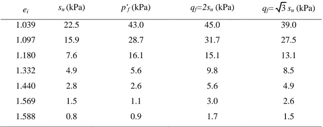
Table 4.4. Estimated stresses at failure from vane shear tests on kaolin samples from this work. ... 34

Table 4.5. First estimate of stresses at failure for data collected from Wood (1985). ... 38

Table 5.1 Kaolin parameters, taken from Llano-Serna (2012) ... 41

Table 5.2 Parameters for the clayey column collapse simulation ... 46

Table 5.3 Meshing schemes and computational time ... 49

Table 6.1 Geometric model details in MPM simulation of the Tokai-Hokuriku Expressway landslide ... 52

Table 6.2 Mechanical parameters used in the Tokai-Hokuriku Expressway landslide model 53 Table 6.3 Geometric model details in MPM simulation of Vajont landslide ... 58

Table 6.4 Mechanical parameters used in the Vajont, landslide model. ... 60

Table 6.5. Discretisation details in the MPM model ... 67

Table 6.6. Mechanical parameters adopted in Alto Verde ... 67

LIST OF FIGURES

Fig. 2.1. MPM discretization: (a) initial two-dimensional example, and (b) two-dimensional

MPM approximation (Brannon, 2014). ... 7

Fig. 2.2. Schematic illustration of the cone indentation. The left-hand side represents the analysis by Koumoto & Houlsby (2001), and the right-hand side represents finite element analysis results by Hazell (2008). ... 11

Fig. 3.1. The critical state concept for isotropically consolidated soils. Taken from Mayne (1980) ... 16

Fig. 3.2. Stress state during different strength testing; (a) CU-CTC; (b) Mini-Vane test ... 18

Fig. 3.3. Illustration of the iterative process to determine critical state parameters. ... 21

Fig. 4.1. Equipment used (a) Fall cone test; (b) Mini-vane shear test. ... 22

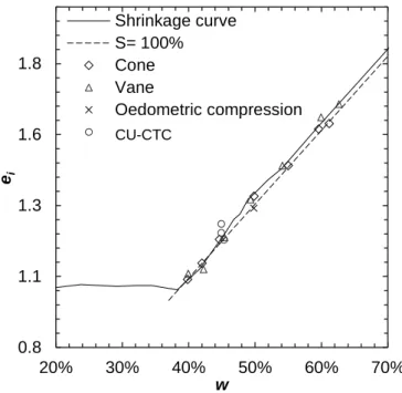
Fig. 4.2. Initial void ratio of the samples employed in this work for different tests. Comparisons against the shrinkage curve. ... 24

Fig. 4.3. Correlation between undrained shear strength su and cone penetration h from test results in this work and results from the literature: (a) all data sets, and (b) zoom near the initial part of the graph. ... 26

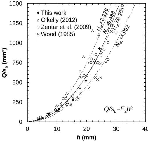
Fig. 4.4. Normalised cone weight Q/su versus final penetration depth h. ... 28

Fig. 4.5. Fall cone factor K versus bearing capacity factor Nch for a range of  values. ... 29

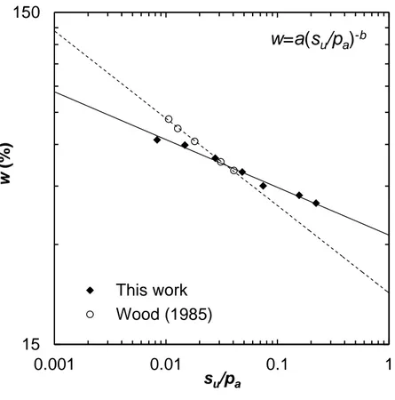
Fig. 4.6. Relationship between undrained shear strength and gravimetric moisture content. .. 31

Fig. 4.7. Oedometer test results for kaolin also used in the fall cone test. ... 32

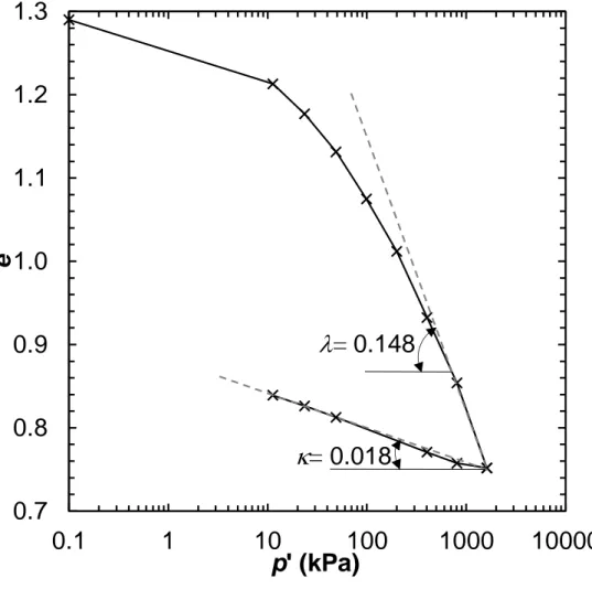
Fig. 4.8. Void ratio-log p‘ curve for determining the CSL. ... 33

Fig. 4.9. Critical state line in q-p’ space. Both modes of undrained failure (mini-vane shear and CU-CTC tests) are represented. The first estimates are represented by open symbols and dashed lines, and the final results are represented by solid lines and black symbols. The values in parenthesis indicate cs. ... 35

Fig. 4.10. Normalised stress-strain curves of CU-CTC test for kaolin. ... 36

Fig. 4.11. Comparison between the results from the proposed methodology (=2) and CU-CTC effective stress paths. The values in parenthesis indicate cs. ... 37

Fig. 4.12. Void ratio-log p‘ curve for CSL determination using data from Wood (1985). Open circles stand for the projections performed for each sample. Closed symbols indicate the final position of the critical state line. ... 38

Fig. 4.13. Initial and final estimates of the linear relationship between deviatoric stress and mean effective stress for data collected from Wood (1985). The values in parenthesis indicate cs. ... 39

Fig. 5.1. Discretisation strategy adopted for the simulation: (a) Surface-based cone discretisation; (b) Cone shell adopted to minimise the number of material points (Llano-Serna, 2012) ... 41 Fig. 5.2. Sample 4: Penetration stages in tridimensional MPM cone penetration. The color map indicates the stress level ratio active failure

vM vM

SL=  . ... 43 Fig. 5.3 Comparison between experimental and numerical results: (a) Relationship between penetration depth and undrained shear strength; (b) Sample 3: Time variation for experimental and numerical tests; (c) Sample 3: Theoretical, analytical and experimental velocity of the fall cone test. ... 44 Fig. 5.4. Collapse of clayey columns via the MPM: (a) aspect ratio a= 0.5; (b) a= 7.0. ... 46 Fig. 5.5. Normalized final height and width of clayey columns as a function of the aspect ratio (a) normalized height; (b) normalized width. ... 47 Fig. 5.6. Schematic diagram of a synthetic slope for numerical simulations, the height, is variable. ... 48 Fig. 5.7. Relationship between the horizontal displacement in the top of the slope and slope height for different geometries. ... 49 Fig. 5.8. Mesh discretization and final deformations of a 5 m high 45° slope using numerical methods: (a) FEM; (b) MPM ... 50 Fig. 5.9. Deviatoric strain in a 5m height 45° slope using numerical methods: (a) FEM; (b) MPM. ... 50 Fig. 6.1. MPM numerical model of the cross section of the Tokai-Hokuriku Expressway. .... 51 Fig. 6.2. Change of kinetic energy as a function of time in the Tokai-Hokuriku Expressway landslide. ... 53 Fig. 6.3. Evolution of the surface configuration and kinetic energy released during the Tokai-Hokuriku Expressway landslide. ... 54 Fig. 6.4. The final surface configuration of the Tokai-Hokuriku Expressway landslide. The thick yellow arrows indicate a zone of debris accumulation along the failure surface. ... 55 Fig. 6.5. Panoramic view of the Tokai-Hokuriku Expressway slope failure. Modified from Ye (2004). The thick yellow arrows indicate an observed zone of debris accumulation modelled in Fig. 6.4. ... 55

Fig. 6.6. Panoramic view of the Vajont landslide. (a) Landslide crown and analysed cross-section (b) Concrete arch dam. Modified from Barla and Paronuzzi (2013). ... 56 Fig. 6.7. Geological section adopted in this research for the Vajont landslide before 9 October 1963. Taken from Paronuzzi & Bolla (2012). ... 57 Fig. 6.8. MPM numerical model of the 1-1‘ cross section in the Vajont landslide. See Fig. 6.6 (a) for cross section location. ... 58 Fig. 6.9. Change of kinetic energy on the failed rock strata as a function of time in Vajont landslide. ... 59 Fig. 6.10. Evolution of the surface configuration and kinetic energy released during the Vajont landslide. ... 61 Fig. 6.11. Vajont final surface configuration. ... 62 Fig. 6.12. Relationship between material point size and model height for slope stability problems. ... 63 Fig. 6.13. Satellital images adapted from Google Earth (Llano-Serna et al., 2015). ... 64 Fig. 6.14. Panoramic picture. The left-hand side picture shows the situation the day of the landslide. Right-hand side three years later (Llano-Serna et al., 2015). ... 65 Fig. 6.15. Close-up picture of the landslide crown (Llano-Serna et al., 2015). ... 65 Fig. 6.16. Soil profile and general characteristics at A‘-A cross-section (Llano-Serna et al., 2015). ... 66 Fig. 6.17. MPM model adopted for Alto Verde landslide (Llano-Serna et al., 2015). ... 67 Fig. 6.18. Change of kinetic energy as a function of time in Alto Verde landslide (Llano-Serna

et al., 2015). ... 69

Fig. 6.19. Alto Verde landslide progression with the time (Llano-Serna et al., 2015). ... 70 Fig. 6.20. Alto Verde residential complex guardhouse (Llano-Serna et al., 2015). ... 71 Fig. 6.21. Relationship between the structure vulnerability and the debris depth for different run-out velocities (Llano-Serna et al., 2015). ... 73 Fig. 6.22. Probability of one person being injured of different degrees. Modified from Ragozin & Tikhvinsky (2000). ... 74

LIST OF SYMBOLS

a Acceleration vector

ch

N Bearing capacity factor  Compressibility coefficient

K Cone factor

Q Cone weight

M Critical state strength parameter

q Deviatoric stress

ud

s Dynamic undrained shear strength

'

p Effective mean stress

1, 2

F F Empirical cone fit factors

ext n

f External force in a vertex

b External forces vector

h Fall cone penetration depth

d Final height of the soil column

h Final width of the soil column  Frictional coefficient

0

d Initial height of the soil column 0

h Initial width of the soil column int

n

f Internal force in a vertex

p

m Material point mass

norm n

f Normal force in a vertex

 Parameter accounting for the stress state

 

 Particle characteristic function

p

q Rate of linear momentum in a material point

 Relationship between static and dynamic undrained shear strength

S Saturation

 Scalar field of density  Second order stress tensor

s

G Specific gravity of the grains

u

s Static undrained shear strength

t Surface forces vector tan

n

f Tangential force in a vertex

 Tip cone angle



 

 

S x Matrix storing the shape functions

 

1. INTRODUCTION

In Geotechnical Engineering, a number of large deformation problems arise and some are still unsolved to date. Some typical examples include field testing like SPT, CPT, DMT; laboratory testing such as vane test, fall cone test; and practical applications, for instance, the run-out processes during landslides and pile driving. These problems are very hard to simulate numerically. The main reason is the difficulty to properly assess the geometry changes due to loads and different boundary conditions. Another challenge is the accurate representation of material behaviour. To exemplify the complexity in a typical geotechnical problem, the simulation of a pile that is driven into the ground is mentioned. The goal of a practitioner is to calculate the bending moments needed for the design of piles in addition to quantifying the bearing capacity produced by the friction between pile and ground. The difficulty in this problem is quite high because severe deformations occur and the material is subjected to extreme strains causing compactions and localised failure due to stresses reaching upper limits.

1.1 MOTIVATION

The main motivation for this research are the limitations of using traditional and widely used numerical methods such as the Finite Element Method (FEM) to solve large deformations problems. On the other hand, in the geotechnical engineering practice, it is very frequent the occurrence of stiff objects (e.g. piles or rods with different tip shapes) indenting a softer media (soil) or even the case of large scale masses deformation such as in landslides. A common factor in these cases is the rapid loading rate, generally leading to undrained condition.

To shed light on this subject, the scientific hypothesis defended in this thesis establish that a large deformation problem such as observed in an indentation problem or landslides subjected to fast load frames, may be solved using the Material Point Method (MPM) adopting a mixed Eulerian-Lagrangian framework.

1.2 OBJECTIVES

The main objective of this research is the simulation of problems involving large strains, such as indentation problems and large-scale landslides. Furthermore, the thesis also focuses on the behaviour of soils subjected to rapid loadings described by an undrained condition. For this

purpose, the Material Point Method (MPM) is used taking advantage of a mixed Eulerian-Lagrangian formulation.

To attain this goal, the thesis trills a series of specific objectives as shown therein.  Testing of a computational program, based on the Material Point Method;

 Simulation of a cone penetration problem, subjected to its weight, in a saturated soft clay mass under undrained conditions;

 Development of a methodology to estimate soil parameters for normally consolidated clays in undrained conditions, based on simple tests, such as the fall cone test and the mini vane shear test;

 Simulation of real large-scale landslides and comparison with field observations and literature reports.

1.3 METHODOLOGICAL FRAMEWORK

The focus of the approach and methodology begins with a literature review that shows the main aspects of the Material Point Method, the fall cone test as a typical example of penetration problem in geotechnics and run-out process during landslides. Next, it is performed the installation and testing of NairnMPM, an open source code from Oregon State University.

As part of the laboratory work, it was performed a series of test in industrial kaolin clay. The laboratory tests included the widely known fall cone test and mini-vane in clay samples for different water contents.

Based on the results obtained in the characterization phase, it was possible to establish, a simple calibration procedure for the fall cone apparatus using the relationship in the model proposed by Hansbo (1957).

Furthermore, the calibration results and its relationship with the shear strength characterization allowed us to develop a simplified methodology to obtain advanced material parameters, based on simple laboratory tests.

Back to numerical modelling, the fall cone test is modelled using the Material Point Method to assess the applicability of the computational tool to solve large deformation and movement of soil masses.

The application of the Material Point Method is later extended to the simulation of large scale run-out processes in landslides such as observed in Vajont and Tokai-Hokuriku

Expressway. Then, an application of the framework of risk assessment for landslides is also introduced.

Finally, we present the concluding remarks of the research with the outlook to future work. Besides this thesis, the present study produced the following list of publications:

1. An assessment of the material point method for modelling large scale run-out processes in landslides (Llano-Serna et al., 2015).

2. A Simple Methodology to Obtain Critical State Parameters of Remolded Clays Under Normally Consolidated Conditions Using the Fall Cone Test (Farias & Llano-Serna, 2016). 3. Numerical modelling of Alto Verde landslide using the Material Point Method

(Llano-Serna et al., 2015).

4. Numerical, theoretical and experimental validation of the material point method to solve geotechnical engineering problems (Llano-Serna & Farias, 2015).

5. Simulations of fall cone test in soil mechanics using the material point method (Llano-Serna et al., 2016).

1.4 THESIS OUTLINE

The reminder of the thesis is structured as follows. Chapter two introduces the background and basic concepts that are relevant in the context of the thesis. It begins by discussing how large strain problems are traditionally addressed and the limitations of the state of the art. Moreover, a historical description of the development of the MPM is followed by the basic equations that describe the method and the use of MPM in geotechnics.

Still, in the second chapter, it is addressed the description of the fall cone test and basic concepts of landslides which are the main topics addressed in the research.

The third chapter is one of the most interesting results of the research. It is related to the fact that critical state parameters may be estimated conveniently from a simple test such as the falling cone. The procedure developed and described show how a simple calibration procedure allows approximating critical state parameters within a precision of around 20%.

Chapter four summarizes the materials and methods used in the experimental campaign. It also applies and validates the methods described in chapter three. This is one of the most valuable findings of the research; it complies an improved interpretation and calibration of the fall cone test.

In the fifth chapter is presented the numerical validation of the material point method (MPM) to solve large strains problems. The numerical validation is focused on the simulations of the fall cone test presented previously. The simulations are verified against

laboratory results including the evolution of penetration with time. Additionally, validation exercises were also performed in regards of the horizontal deformations of a synthetic slope and the collapse of a soil column. The simulations compare well with experiments available in the literature. The code used and the numerical simulations were able to capture all the main features of the problems analysed herein and proved to be a convenient tool to tackle this kind of problems.

In chapter six it is demonstrated the predictive capabilities of the MPM for the simulation of run-out processes during landslides. The approach is focused on the post-failure behaviour and in particular, to the computation of important quantities such as run-out distance, maximum velocity, and energy release. The validation is conducted based on simulations of two case studies of different scales, namely the Tokai-Hokuriku Expressway failure in Japan and the Vajont landslide in Italy. The results show a very good agreement with field and other numerical observations. Finally, the methodology is applied to a real case problem where the outputs of the MPM simulations are used as a tool in the quantification of risk.

Chapter 8 concludes the thesis by providing a summary of the outcomes and presenting an outlook for future studies.

2. LITERATURE REVIEW

When a continuum body is on movement, its state variables (e.g. stress or temperature) may change with time. These changes may be described by two mathematical approaches (Lai et al., 1993). The first method tracks the ―elements‖ comprising the continuum as they move in space and time. This approach is widely known as the Lagrangian frame of reference. Lagrangian approaches are mostly used in solid mechanics and numerical methods such as the Discrete Element Method (DEM). The second approach considers the changes of the state variables in fixed positions and is known as a spatial or Eulerian frame of reference. In Eulerian methods, the change of the stress state, for example, is measured in a fixed point of the medium as a function of time. Note for instance that a single space position may be occupied by different particles for changes in time. This approach is mostly used in fluid mechanics.

2.1 FINITE ELEMENTS FOR SOLVING LARGE DEFORMATIONS

The numerical modelling both in industry and academy is mainly dominated by the use of the Finite Element Method, FEM (Augarde & Heaney, 2009). However, the traditional formulation of the FEM does not provide a solid framework to solve large strain problems. Moreover, FEM may present numerical instabilities such as mesh entanglement when significant strains are experienced.

As an alternative, and preserving the basic concept of FEM an updating of the Lagrangian discretization was introduced (Bathe et al., 1975). This process is called re-meshing and involves the mapping of the stress variables from the deformed mesh to a new mesh introducing errors in the converged solution (Wieckowski et al., 1999).

Recent FEM formulations show a good performance solving complex problems, building sequences or non-linear constitutive models under bi-dimensional conditions. However, the framework presents issues in three-dimensional models when mesh generation, re-meshing, different soil layers or curved interfaces are involved (Augarde & Heaney, 2009).

2.2 NUMERICAL METHODS APPLIED IN FINITE DEFORMATION PROBLEMS

The modelling of large deformation problems is not straightforward. The complexity of the phenomena relies on the severe deformations that cause compactions and localised failure due to stresses reaching upper limits. Recent advances in computational capacity allow the use of

the so-called particle based methods to tackle these problems. The most popular choices include the discrete element method (DEM) developed by Cundall & Strack (1979); the smoothed particle hydrodynamics (SPH) (Gingold & Monaghan, 1977); and the MPM derived for solids by Sulsky et al. (1994).

In the DEM each material grain is considered independently; thus the macroscopic properties cannot be directly calibrated as it would be expected for a method based on classical mechanics, also, is nearly impossible to model the correct number of elements (grains) in a geotechnical problem (Boon et al., 2014). On the other hand, SPH and MPM are derived from a continuum mechanic framework that allows the use of conventional geotechnical constitutive models. Nevertheless, many geotechnical problems involve boundary interfaces, and SPH may cause loss of consistency in such cases. Furthermore, the use of stabilization techniques seems to be necessary to achieve convergence (Bandara & Soga, 2015). In MPM, accuracy may also be lost due to extrapolations and interpolations in the auxiliary grids needed for the enforcement of balance of momentum. A detailed description of large-deformation methods common in solid mechanics and geotechnical engineering is also available in Li & Liu (2004) and Soga et al. (2016)

2.3 BACKGROUND AND FORMULATION OF THE MATERIAL POINT METHOD

The original development of the MPM was called particle-in-cell (PIC) by Harlow (1964). Later it was first applied to fluid dynamics by Brackbill & Ruppell (1986). Sulsky et al. (1995) developed the first extension of the method for solid mechanics and called it MPM. Today, one of the most used approaches of the MPM is the generalization of the framework developed by Bardenhagen & Kober (2004). It is called Generalized Interpolation of Material

Point Method (GIMP), and the idea was to solve numerical noises produced by the transit of

material points across cell boundaries.

The basic principle behind the MPM is depicted in Fig. 2.1. MPM discretization: (a) initial two-dimensional example, and (b) two-dimensional MPM approximation (Brannon, 2014).Fig. 2.1. Fig. 2.1 (a) shows an object to be analyzed using the MPM overlapped with the yellow grid. The object is then converted or transformed into a red dot numerical representation that is unique, as shown in Fig. 2.1b called material elements. The discretised object is then ready to be analyzed. Its movement will depend on the direction of the movement of each material point, and the gridlines surrounding each material point will move according to the movement of the sphere. The material points move with the integration of

time on a fixed Eulerian grid. Recently, it has been found that the numerical framework provided by the MPM is suitable for modelling landslide and penetration problems. The main advantage of using the MPM is that material flow is allowed by a solid Eulerian-Lagrangian approach. Also, it allows for solid mechanics constitutive models. Thus, the traditional formulations of soil mechanics are still valid, enhancing the applicability of the MPM (Soga et al., 2016).

(a) (b)

Fig. 2.1. MPM discretization: (a) initial dimensional example, and (b) two-dimensional MPM approximation (Brannon, 2014).

The numerical method used in this work is fully described by Buzzi et al. (2008) and is based on the generalised version of the Material Point Method (Bardenhagen & Kober, 2004). At a local basis, the Master Dissertation published by Llano-Serna (2012) describes in detail the derivation of the numerical method, and here we discuss the main points.

2.3.1 FORMULATION

The balance of linear momentum at any point of a continuum body is described by

 

div  ba (2.1)

where  is the second order (total) stress tensor, ―div‖ is the divergence operator,  is the scalar density field, b is the vector of external body forces, and a is the acceleration vector at the point under observation.

To achieve a numerical solution, the weak form of the balance of linear moment is obtained by means of the weighted residuals method. The equation (2.1) is thus multiplied by arbitrary test functions and integrated over the initial volume. Further, by applying integration by parts and employing the Green-Gauss theorem, the following equation is obtained

: A V V V dw w tdA w bdV dV w adV dx         









where t represents the vector of tractions applied to some part of the surface. Therein, w x

 

In the MPM, equation (2.2) is discretised considering the vertices of the background grid and a material point, resulting in

p p np n p np p np p A p p V  G _ S tdA m bS _ q S    



_





where the subscript ―p‖ denotes a material point, ―n‖ denotes a vertex (node) of the computational grid and q the vector of linear momentum. Summation over all material points

or all vertices are denoted by p





int ext

n n n

f



f



q

Furthermore, the internal and external forces are transferred to the vertices using interpolation functions S_n and matrix S . The matrix _np S_np takes a weighted average of function Sn considering only the volume Vp occupied by the material point "p" in the vicinity

of vertex "n". This is computed as follows

 

   



where V*  V V_p represents the support volume of the characteristic function _p that accounts for the contribution of the material points to the computational grid. Each material point is assigned a characteristic function _p that constitutes a partition of unity in the initial configuration ―i‖.

Matrix S_np is also used to extrapolate the rate of linear momentum q_p at the centre of mass of the material point to the grid vertices as shown in the right side of the equation (2.3). The internal forces

f

transfer matrix G . This matrix represents an average of the matrix _np G_n which contains the derivatives of function Sn.

2.3.2 CONTACT

It should be noted most problems involve more than one material, and a contact law between different materials must be adopted. Contact models in the MPM were first developed by Bardenhagen et al. (2001) and later improved by Lemiale et al. (2010) and Nairn (2013). Separate velocity fields are used for each material involved in the simulation. Vertices that received contributions from different types of materials use a contact mechanism to adjust their linear momentum. A normal direction between both materials is calculated and a normal force f_nnorm at a contact point is computed by projecting the linear momentum along this normal direction. Then, the maximum tangential force f_ntan is obtained from a simple frictional model as follows:

tan norm

n n

f    f (2.6)

Therein,  is the frictional coefficient that relates normal and tangential forces. 2.4 MPM IN GEOTECHNICAL ENGINEERING

After the main developments of the MPM at the beginning of the century; it has been used for a wide range of engineering benchmarks, such as a fixed beam deformed under its own weight (Beuth et al., 2007; Beuth et al., 2011); oedometric compression test (Beuth et al., 2007; Zabala 2010); vertical deformations in synthetic slopes (Beuth et al., 2008; Vermeer et

al., 2008); shallow foundations (Ma, 2002; Coetzee, 2004; Raghav, 2005; Zhang et al., 2009);

models including discontinuities (Karuppiah, 2004; Daphalapurkar et al., 2007; Guo & Nairn, 2006) and nano-indentation (Ma, 2002; Raghav, 2005).

More sophisticated geotechnical case studies include the analysis of active and passive earth pressure (Coetzee, 2004; Vermeer et al., 2008; Beuth et al., 2011; Zhang et al., 2009); the local stability of retention walls (Wickowski, 2004; Vermeer et al., 2008; Wieckowski, 2011); collapse of embankments reinforced with geotextiles (Zhou et al., 1999); run-out processes in artificial slopes (Numada et al. 2003; Shin et al. 2010; Andersen & Andersen, 2009, 2010); foundation of dams over soft soils (Zabala, 2010); pull-out testing (Coetzee et

al., 2005); and pile driving (Wickowski, 2004). A detailed discussion of most of these

examples was carried out by Llano-Serna (2012).

The last three years have been very active regarding publications of the MPM used to solve complex geotechnical engineering problems. Some examples include applications in the offshore industry (Al-Kafaji, 2013; Lim et al., 2014; Dong et al., 2015); pile installation

(Lorenzo, 2015; Phuong et al., 2014); slope instabilities due to dynamic forces produced by earthquakes (Abe et al., 2015; Bhandari et al., 2016); and more recently the coupling of the hydro-mechanical problem (Abe et al., 2014; Muller & Vargas Jr, 2014; Soga et al., 2016). However, two main limitations are regarded. In the first place, there are very few examples of real-scale applications fully validated, and in second place, most of the publications are focused on the descriptions of phenomena. Very limited applications of the new features provided by the MPM are discussed.

2.5 THE FALL CONE TEST

In the present study, the most popular fall cone method is considered, i.e. the British cone with a 30° tip angle and mass of 80 g. The fall cone equipment complies with the British Standards (BS 1377-2, 1990). The test starts with the cone tip touching the soil surface and then it is released to fall freely under its own weight. The final penetration depth of the cone is registered after 5s.

Hansbo (1957) established one of the most accepted relationships between the undrained shear strength (su) and the cone penetration depth (h) as follows:

2 u KQ s h  (2.7)

where Q is the total cone weight, h is the final penetration depth of the cone, and K is Hansbo´s cone factor.

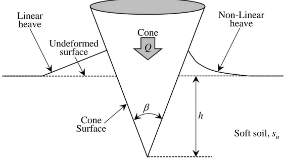
Fig. 2.2 shows a schematic diagram of the final configuration in the fall cone test. According to Koumoto & Houlsby (2001), the load Q at the end of the penetration process can be approximated by bearing capacity theory resulting in:





soil is taken into account, A is the cone surface in contact with the soil, and  is the cone tip angle.

Koumoto & Houlsby (2001) also calculated values of Nch by means of the method of

characteristics, using a linear simplification of the heave (left-hand side of Fig. 2.2). Hazell (2008) applied the finite element method with adaptive meshing to assess the influence of the curved heaved surface on the Nch factor (right-hand side of Fig. 2.2).

Fig. 2.2. Schematic illustration of the cone indentation. The left-hand side represents the analysis by Koumoto & Houlsby (2001), and the right-hand side represents finite element analysis results by Hazell (2008).

By combining the quasi-static and dynamic analyses, Koumoto & Houlsby (2001) expressed the fall cone factor K as:





shear strength (sud) from the fall cone test.

Further studies showed that the bluntness of the cone point has no effect on the K factor (Claveau-Mallet et al., 2012). The equation (2.9) is often used to estimate K based on assumed values for Nch and  or using previous experimental observations. This procedure is

not recommended for the type of cone used here because results from the 30° cone test are highly sensitive to cone surface roughness. Experimental calibration is highly recommended, and this issue is pursued in this thesis.

Despite the above, it is very common in the recent literature to adopt a cone factor from classical or previous references instead applying proper calibration (i.e. Stone & Kyambadde, 2007; Mahajan & Budhu, 2009; Cevikbilen & Budhu, 2011; Vinod & Bindu, 2011; Azadi & Monfared, 2012; Boukpeti et al., 2012; Claveau-Mallet et al., 2012; O‘Kelly, 2012; Das et al., 2013). Calibration procedures are presented by Sharma & Bora (2003), Rajasekaran & Narasimha Rao (2004), and Zentar et al. (2009). However, these lack proper interpretation



under the fall cone test theory. Classical works by Hansbo (1957), Karlson (1977), Wood (1982) and Wood (1985) can also be found; some of these results will be discussed later.

2.6 NUMERICAL MODELLING OF LANDSLIDES (THE RUN-OUT)

The increase of urban activities near or in mountainous areas requires more attention to the mitigation of threats due to landslides. Landslides are caused by hydrological, environmental, or anthropogenic changes. Due to the potential velocity, impacting forces or run-out distances, a slope failure may result in large movement of mass with serious consequences to people and infrastructure. Even if a potential landslide can be predicted, it remains the question on how far the debris can travel. The answer is critical to prevent further losses and mitigate the hazard by the use of protection barriers (Kishi et al. 2000; Peila & Ronco 2009; Shin et al. 2010; Brighenti et al. 2013; Mast et al. 2014). Another important step is the quantification of the force imparted by the landslide (Ashwood, 2014) to optimize engineering structures and barriers.

According to Skempton & Hutchinson (1969), a landslide involves three stages: (i) pre-failure deformations; (ii) the pre-failure itself; and (iii) post-pre-failure displacements or deformation. The degree of shear resistance loss during failure determines the velocity of the run out. This failure stage also involves kinematic changes from sliding to flow or fall, which is also relevant to the post-failure behaviour and destructiveness of the landslide (Hungr et al., 2014). Slope stability analysis in geotechnical engineering practice is currently focused on establishing the pre-failure state and determining the physical conditions that may trigger the slide. Typical analyses use limit equilibrium methods, plastic limit theorems or the finite element method (FEM) (e.g. Hughes, 1984; Griffiths & Lane, 1999; Belytschko et al., 2013; Zienkiewicz & Taylor, 2013).

The pre-failure state of a slope is usually assessed by quantification of the so-called Factor of Safety (FOS). However, the traditional approach of slope stability analysis disregards the potential consequences of a landslide. The most recent approaches from a technical point of view are focused in the quantification of risk (Coelho-Netto et al., 2007; Uzielli et al., 2008, 2015; Jaiswal et al., 2010; Li et al., 2010), and monitoring, analysis and forecasting of hazards (Dai et al., 2002; Ho & Ko, 2009; Calvello et al., 2015). As described before, the MPM features make it very attractive to evaluate the consequences of large deformation processes as in rapid landslides. Thus, the analysis presented in this research will be focused on the predictive capabilities of the method to estimate the consequences of a landslide. More traditional approaches (e.g. FOS quantification) are then disregarded.

The only real case study using the MPM found in the literature is the work by Andersen & Andersen (2009) on a landslide near Lønstrup, Denmark, in 2008. Therefore, this work aims at further exploring the capabilities of the MPM for modelling real landslides.

Total stress analysis incorporated in the current MPM is appropriate for the post-failure analysis of slopes. Nevertheless, a more detailed approach may be possible using effective stress analysis considering the liquid-solid interaction. Some novel examples to solve the resulting coupled formulation can be found in Pedroso (2015a) and Pedroso (2015b) where the mixture theory has been applied considering each constituent (e.g. liquid and solid). As a consequence, mass balance equations must be solved, and the process is slower. The effective stress analysis of landslides with MPM is a future topic outside the limits of this thesis. To this end, other aspects such as dealing with some limitations due to post-failure behaviour (Abe et al., 2014; Bandara & Soga, 2015) must be investigated as well.

Other alternative techniques that allow for a proper geometrical and constitutive representation of run-out processes exist as well, although mostly based on computational fluid dynamics such as the works by Hungr (1995); McDougall and Hungr (2004); Sawada et

al. (2004); Ward & Day (2011); Vacondio et al. (2013); Chen & Zhang (2014); Sawada et al.,

(2015). The run-out model specific to solid mechanics includes the work by Lo et al. (2013); Zhang et al. (2013); Pastor et al. (2014); Sassa et al. (2014); Boon et al. (2014) and Albaba et

al. (2015). However, as Mast et al. (2014) states, the main drawback with some these

alternative methods are related to the scale of the domain and even the constitutive models derived for Non-Newtonian fluids. Finally, empirical and analytical methods are also available as described by Hungr et al. (1984) and Corominas (1996); however, they have many limitations.

3. PROPOSED METHODOLOGIES FOR THE CALIBRATION OF

CONE PENETRATION TESTS AND OBTAINING CRITICAL

STATE PARAMETERS

In this chapter, it is initially presented a simple methodology to calibrate the so-called cone factor K, proposed by Hansbo (1957), with the aid of mini-vane shear tests. Based on these two tests it is later proposed a simple methodology to obtain the main compressibility and strength parameters of critical state models. The methodologies will be validated in the next chapter.

3.1 THE FALL CONE TEST AND ITS CALIBRATION For the sake of convenience, equation (2.7) is rewritten as:

2 1

u

s F h _(3.1)

where the new factor is simply F1=KQ.

Thus plotting pairs of (h-2, su) obtained experimentally and fitting a linear regression would

readily give an estimate of F1, from which the cone factor K can be directly obtained for a

known value of the cone weight (Q). The values of penetration h can be obtained from cone penetration tests, and the values of undrained shear strength (su) can be obtained from

mini-vane tests with clays in the same conditions. This methodology will be applied later in the thesis.

Koumoto & Houlsby (2001) noted that equation (2.8) could be simplified to: 2

2

u

Q s F h _(3.2)

where the factor F2 can be expressed as:





2

2 ch tan 2

F  N  

(3.3) Comparing equations equation (2.7) and (3.2), it is clear that F2 equals the inverse of factor

K. Therefore, calibration of F2, using experimental pairs of (Q/su, h2) and a linear regression

or (Q/su, h) and a quadratic regression, gives a basis for interpreting the relation between the

cone factor K and the cone bearing capacity factor the Nch.

With a calibrated fall cone factor K, for a given cone, the fall cone test can be used to estimate the undrained shear strength (su) for a range of clayey soils; i.e., the calibration

procedure just needs to be performed once, since the K factor depends only on the cone roughness characteristics. Re-calibration is recommended to check the results.

The methodology to calibrate the fall cone used in this thesis can be summarized as follows:

1. Plot the results of cone penetration (h) and vane shear tests (su), with the value

of h-2 in the abscissa versus su in the ordinates. Later, fit the best straight line through the

origin. It is possible to find the slope F1 and consequently the value of the cone factor K

using equations (2.7) and (3.1);

2. The test data can be fitted applying equation (3.2). Thus, the bearing capacity factor Nch of the cone is determined using equation (3.3);

3. Combining the experimental values of K and Nch, the strain ratio applied by the

cone can be estimated back-calculating  variable from equation (2.9) 3.2 CRITICAL STATE PARAMETERS

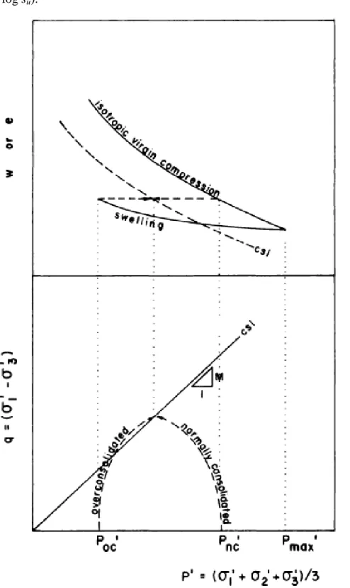
The critical state concept is usually used to predict the undrained strength of clayey soils. For an isotropically consolidated soil that has undergone a load and unload cycle, it may be assumed that the stress path will reach the failure point on the critical state line (CSL). The main idea can be depicted in Fig. 3.1. It must be noted that the isotropic virgin compression curve or normally consolidation curve describes a straight line in a semi-log space usually denoted by . Similarly, the swelling or recompression curve also describes a straight line usually denoted by . These parameters;  and  define de deformability characteristics of the soil whereas the strength is defined by the slope M. This research will focus its effort in the estimation and validation of the material parameters , and M. The Poisson‘s ratio , is assumed constant as 0.499 unless a different value is specified, consistent with undrained conditions for saturated clayey soils. Moreover, the state parameters are disregarded.

Koumoto & Houlsby (2001) proposed a procedure to determine fitting variables a and b related to the traditional critical state parameters. The key assumptions for this computation are briefly described here for the sake of completeness. Furthermore, the theoretical derivations of equations (3.4)-(3.11) are largely the same as Koumoto & Houlsby (2001). However, we show improvements in the procedure for the experimental data interpretation. The following relationship between the gravimetric moisture content (w) and the undrained shear strength (su) is established:

b u a s w a p         (3.4)

where pa is the atmospheric pressure, and a and b are empirical fitting coefficients. These

coefficients can easily be determined from a linear fitting of equation (3.4) in the logarithmic space (log w–log su).

Fig. 3.1. The critical state concept for isotropically consolidated soils. Taken from Mayne (1980)

Parameter a is related to the water absorption, and retention capacity of the soil and b is related to soil compressibility (O‘Kelly, 2013). Combining equations (2.7) and (3.4), the following expression is obtained:

2 K b a Q w a p h         (3.5)

Equation (3.5) can be further extended by considering critical state theory, which establishes the well-known relationships for the Critical State Line (CSL), expressed by:

' ln a a p e e p      _{ }   (3.6)

In the equation (3.6), p’ is the mean effective stress p’=(’1+’2+’3)/3,  is the

compressibility coefficient and ea is the void ratio for p’= pa. A reference pressure pa=100

kPa (1 bar) is usually adopted.

Instead of equation (3.6), Koumoto & Houlsby (2001) proposed the following expression, which is linear in the bi-log (e-p’) space (see also Hashiguchi & Chen, 1998):

' ln( ) ln( )_a ln a p e e p      _{ }   or ' a a p e e p          (3.7)

Using the relationship Gsw=Se, for a saturated condition (S=1, and assuming that the

specific gravity of the pore water is unity), and the gravimetric moisture content w, expressed in percentage, equation (3.7)-b becomes:

' 100 a s a e p w G p      _{ }   (3.8)

where Gs is the specific gravity of the soil particles.

The mean effective stress p‘ can be related to the deviatoric stress qf (index f for failure) at

the critical state according to the following expression:

f q Mp (3.9) where:



 











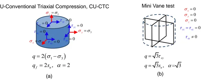
For conventional triaxial compression tests (e.g. CU-CTC, it is consolidated undrained conventional triaxial compression), the stress state is such that x=y=3, z=1 and

xy=yz=xz=0, then q=(1-3) resulting in qf=2su at failure. This is the value used by Koumoto

& Houlsby (2001). However, the normal stresses during the vane shear test are negligible, and the stress state is better represented by x=y=z=0, yz=xz=0 and xy≠0, then q= 3xy and

qf= 3 su at failure, see Fig. 3.2. Both cases are conveniently represented in this thesis by a

relationship between the deviatoric stress qf and the undrained shear strength (su) as follows:

f u

q s (3.11)

where =2, as assumed by Koumoto & Houlsby (2001) for CU-CTC and =√3 for the mini-vane shear test. As a result, M is not constant and depends on the stress and deformation conditions. This is further illustrated in the following section.

Fig. 3.2. Stress state during different strength testing; (a) CU-CTC; (b) Mini-Vane test

It is worth noting that the cross-section of the true failure envelope on a deviatoric plane is circular (von Mises) since the fall cone test is considered to happen under undrained conditions in a clayey soil. Note that drained conditions can lead to different shapes such as the Matsuoka-Nakai criterion (Matsuoka & Nakai, 1974).

Finally, by substituting equation (3.11) into equation (3.9), and the resulting expression for

p‘ into equation (3.8), the following equation is obtained: 100 a u s a e s w G M p     _{ }    _{   }  _{  } (3.12) (a)

CU-Conventional Triaxial Compression, CU-CTC Mini Vane test

1 z   0 zy   0 zx   0 xy   3 x   0 xz   y3 0 yz   0 yx   0 z   0 xy   0 x   0 y   0 yz xz    3 3 , = 3 xy u q q s    





By comparing equations (3.4) and (3.12), the following expressions relating the coefficients a and b and the Cam Clay parameters (ea,  and M) are found:

100 _a s e a G M        _{ }   (3.13) b (3.14)

which are similar to those derived by Koumoto & Houlsby (2001), with the exception of the  factor. With these coefficients and related expressions, the results of the fall cone and vane shear tests can be used to calibrate the deformability and strength parameters of the Cam-clay model as proposed by Roscoe et al. (1958).

The coefficient b, according to the equation (3.14), gives the parameter, whereas the a parameter describes a single equation (3.13) for two unknowns (ea and M); hence an iterative

methodology has to be considered for calibrating the fall cone test.

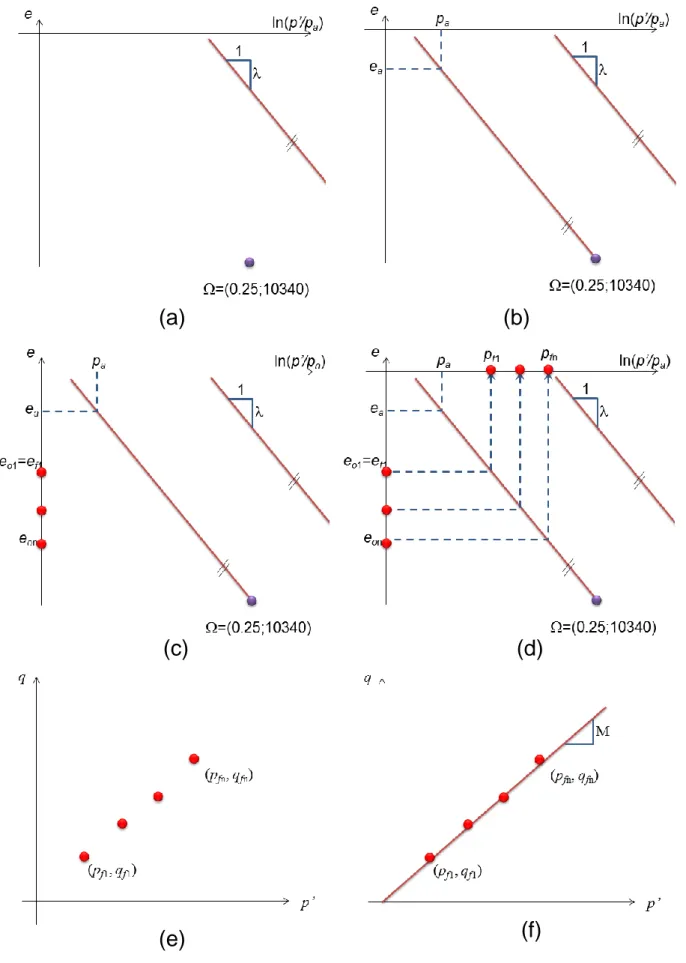
3.2.1 ITERATIVE COMPUTATION OF CRITICAL STATE PARAMETERS

The results of a calibrated fall cone test, or those obtained directly from the vane shear test, can now be used to estimate the position of the critical state line (ea) and its slope (M or cs).

The methodology proposed here to obtain these parameters is described as follows:

1. The process starts by computing the a and b coefficients by fitting the test data according to the equation (3.4) and exploring the relation w - su. Note that, from

equation (3.14), b corresponds to slope of the NCL, i.e., the virgin compressibility coefficient (See Fig. 3.3 (a)

2. The slope of the critical state (, assumed parallel to the NCL, is already determined. Thus the CSL becomes completely determined if a point = (e, p) is

selected – the initial guess for this point is discussed in Section 4.2See Fig. 3.3 (b); 3. Using the values of  and =(e, p) in equation (3.6), the value of the void ratio (ea) for the reference pressure (pa) is establishedSee Fig. 3.3 (b);

4. Because the samples in the fall cone test and the vane shear test are considered undrained, the initial and final void ratios ei are equal to each other at failure; hence

5. Using the values of void ratio (ef =ei) and the CSL equation, the values of

mean effective stresses at failure (p’f) are obtained using equation (3.6). See Fig. 3.3

(d);

6. Now, for each initial void ratio condition, the corresponding deviatoric strength (qf) is obtained from the computed (or experimental) undrained shear strength (su) via

equation (3.11). See Fig. 3.3 (e);

7. With p’f obtained as in step 5 and qf from step 6, the best linear regression

through the origin and fitting the points (p’f, qf) is computed. Then, the slope M of the

critical state line is obtained, and the corresponding friction angle at critical state (cs)

can be readily calculated by means of (see Fig. 3.3 (f)):

1 3 sin 6 cs M M  _     _   ; (3.15)

8. By using the computed value of the slope M (and ), a new ea is obtained

considering the coefficient a from step 1 via equation (3.13). This means that a new position of the CSL based on the new value ea is established;

9. Finally, by comparing the new reference void ratio ea with the value previously

estimated the process is repeated from step 2 if the difference is not acceptable. In step 2, last computed value of ea is the input value. Iterations are performed until

convergence on ea (smaller than a tolerance) is obtained.

A Matlab routine for solving the algorithm is included in Appendix A of the thesis.

Note that the derivations presented here do not account for the effect of anisotropy on the undrained shear strength, this means that the procedure applies for remoulded soils. This limitation is not severe when considering critical state conditions because a remoulded soil can constitutively be described by residual parameters.

Note also that equation (3.15) is valid in CU-CTC conditions only; the relationship between M and cs varies with the Lode angle (conveniently observed in the octahedral

plane). Here, it is assumed that M is constant as in the classical Cam-clay model. Nonetheless, more appropriate failure criteria are available in literature such as Matsuoka & Nakai (1974).

Fig. 3.3. Illustration of the iterative process to determine critical state parameters.

(a)

(b)

(c)

(d)

4. LABORATORY TESTING

The main objectives of the laboratory tests described in this Chapter were to generate data for the calibration of cone penetration apparatus and to test the proposed methodology to obtain critical state parameters of saturated clays. The cone penetration results are also used to verify the ability of the MPM to simulate this type of indentation problem in the next chapter. The fall cone measurements comply with the procedures described in the British Standards (BS 1377-2, 1990), see Fig. 4.1(a).

(a) (b)

Fig. 4.1. Equipment used (a) Fall cone test; (b) Mini-vane shear test.

Commercial kaolin clay was used in all tests. The following tests were performed besides the falling cone: material characterization; mini-vane shear; consolidated undrained conventional triaxial compression (CU-CTC); and one-dimensional consolidation.

The mini-vane shear tests follow the standard ASTM D 4648M (2010), see Fig. 4.1(b).. The vane shear apparatus is equipped with a calibrated spring and a dial gauge to measure the

angular strain. The vane blades are 13 mm in height and width. Seven moisture contents ranging from w=40% to w=63% were considered, see Table 4.1; three soil samples per each moisture content were tested for repeatability. Hence, three fall cone and three vane shear tests were performed, and the average results were analysed. To avoid bias errors, all tests were performed with the same equipment and by the same operator.

Table 4.1. Water content for each one of seven tested samples.

Sample Water content (%)

1 40 2 42 3 45 4 50 5 55 6 60 7 63

To further asses the proposed calibration procedure, data from other authors performing similar tests with the 30° fall cone test and mini-vane shear tests were compared. A classical reference involving Speswhite kaolin and the Cambridge Gault clay was considered (Wood, 1985). It is important to note that there are three main differences between the tests described herein and those found in Wood (1985):

1. The fall cone used by Wood (1985) was wiped with an oily cloth before the test in order to minimise soil-cone friction. This practice is not considered in the BS 1377-2 (1990) standard and has consequences as discussed later.

2. The fall cone used by Wood (1985) had a mass of 100 g instead of the standard 80 g; however, this is less critical since the main expressions presented in this work take into account the cone weight.

3. The geometry of the vane shear blades used by Wood (1985) is different to that used in the present tests; however, the mechanisms and deformation rates are comparable.

More recent results are also considered, such as tests on kaolin and organic sediments gathered in northern France by Zentar et al. (2009), and tests performed by O‘Kelly (2012)