Osmotic stress on concentrated colloidal suspensions: a path towards equilibrium?
A.S. Robbes(*,**), F. Cousin (*), and G. M´eriguet(**)
(*) Laboratoire L´eon Brillouin, CEA-CNRS, CEA-Saclay, 91191 Gif-sur-Yvette, France and (**) Laboratoire des Liquides Ioniques et Interfaces Charg´ees, CNRS UMR 7612,case 63,
Universit´e Pierre et Marie Curie, 4, Place Jussieu, 75252 Paris cedex 05, France∗ (Received on 1 July, 2008)
We discuss in this study the advantages and limitations of the osmotic stress method that enables to set the osmotic pressure to a given system. By investigating aqueous suspension of monodisperse silica nanoparticles of radius 78 ˚Aat an ionic strength of 10−2mol/L, we show that the method is very accurate to probe the phase behavior of colloidal suspensions because it allows to prepare samples all along the equation of state of the system at constant ionic strength without any aggregation and with a well defined structure, as shown by Small-Angle Neutron Scattering (SANS) experiments. However the method fails to yield crystalline structures, since solid samples obtained are always glassy, even when the fluid-solid transition is crossed with small successive jumps of 1000 Pa. This phenomenon comes from the kinetics of the process which exhibits in our experimental conditions an exponential decay time with a characteristic time of≈3 hours that induces a very strong change of the volume fraction of the suspension in the early stages of the stress. When the jump of pressure is very important, the system is frozen in the vicinity of the dialysis bag and forms a dense shell that eventually prevents some spatial regions of the sample to reach equilibrium. In this case, the osmotic stress forces the sample to get a structure very spatially heterogeneous at macroscopic scale.
Keywords: osmotic stress, colloidal suspensions, SANS.
I. INTRODUCTION
For more than fifty years, there has been a constant inter-est for the study of the phase behavior of colloidal suspen-sions, both from the theoretical and the experimental points of view. Apart from the industrial applications, this inter-est for colloidal suspensions is mainly driven by the fact that they are very good model systems. First of all, they perfectly mimic atomic system in the framework of the so-called ’one-component model’ where the colloidal nanoparticles are con-sidered as objects and the solvent as a continuum medium that only acts on the interparticle interaction [1]. The volume fraction of nanoparticlesφcan thus directly be identified with the densityρ and the osmotic pressure∏ with the pressure P. But the shape and amplitude of the interparticle potential in colloidal suspensions can be very easily tuned experimen-tally within a very large range by simply playing on exper-imental parameters such as pH or ionic strength for electro-statically stabilized systems. Second, they allow to consider objects with an anisotropic shapes as 1-D rods [2] or 2-D discs or platelets [3] which are experimentally available and which display richer phase diagrams than pure spheres [4, 5]. They can for example present nematic or smectic phases at high volume content. There are nevertheless two main dif-ferences between colloidal systems and atomic systems: (i) at very short range the Van der Waals attractive forces are al-ways dominant in colloidal systems and have to be overcome by repulsive forces to reach ’stable’ colloidal state otherwise they drive the system to irreversible aggregation and thus do not always allow to explore all the phase spaces (ii) the struc-tural relaxation time of an objectτr≈R2/D(with R the radius of object and D its self-diffusion coefficient), that is the time taken by an object to diffuse on a typical length of its size, is typically 109higher for colloidal systems than atomic ones
∗Electronic address:[email protected]
which lead to very long times to reach equilibrium in colloidal systems (up to several days..) [1].
The experimental difficulties for the study of phase behav-ior of colloidal systems arise when one wants to study high
φphases (crystals, glasses, nematics) and concentrate the ob-jects while controlling the other parameters. The concentra-tion by solvent evaporaconcentra-tion cannot be used because it implies huge gradients, possible irreversible aggregation and above all, it does not allow keeping constant the physico-chemical parameters that play on the interactions (pH, salinity, poly-mer in solution for sterically stabilized systems). Thus his-torically all the first experimental studies that have dealt with the highφand that have shown the possibility to make col-loidal crystals [6–9] have concerned objects with a typical size of a few hundreds of nm or more. In such systems, the size of the objects is large enough to enable the system to slowly sediment with time owing to the gravitational forces, which enable a very progressive concentration of the system. But this way to concentrate systems cannot be used for sys-tems involving objects of around 10 nm because in this case the gravitational energy is much lower than kT. Such systems have nevertheless a great interest compared to larger system because these are the only ones for which the typical ranges of interactions (depletion range of sterically stabilized systems, magnetic dipolar interactions in ferrofluids, electrostatic re-pulsions) are of the order of size of the objects. This en-ables to get very rich behaviors such as gas-liquid transitions [10, 11], eventually associated with a critical point [12].
poly-mer and fixes the chemical potential of water. Since water and ions can cross the dialysis bag, the reservoir finally imposes its osmotic pressure to the colloidal suspension for a given set of electrostatic physico-chemical parameters. The finalφ
of the colloidal suspension has simply to be measured after-wards. This way of controlling the osmotic pressure of any aqueous suspension is unique and is thus now very popular. It has been used these last years to prepare aqueous suspen-sions of silica spheres [14], clays [15], ferrofluids [16][17], and even binary mixtures [18].
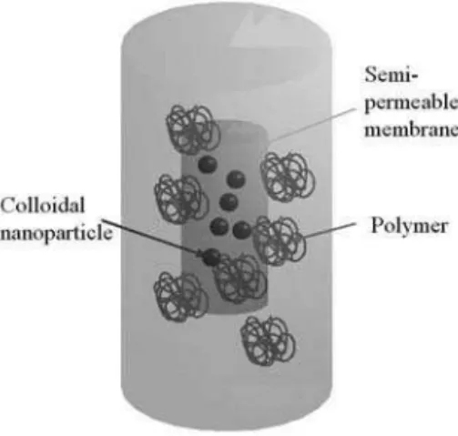
FIG. 1: Principle of an osmotic stress experiment. The nanoparticles are placed in a bag made of a membrane only permeable to water and small ions in a reservoir containing a polymer which osmotic pressure only depends on its concentration. See text for more details.
But the principle of preparation of sample by osmotic stress may prevent to explore the whole space of phases for the study of solid samples, crystals or glasses, starting from di-lute samples. It is indeed possible that the sample preparation leads to the vitrification of the system if the kinetics of the stress, driven by the chemical potential of water, is faster than the kinetics of the colloidal objects to reach equilibrium. In other words, does the osmotic stress freeze the system and trap it in configurations that do not enable to compare ex-periments to the theories or simulations that predict glasses or crystals depending on parameters such as volume frac-tion [19] or polydispersity [20]?
We address this question in this paper by studying the structure of vitreous samples on a model system made of monodisperse nanospheres with a radius of≈7.5 nm dis-persed in aqueous media. We choose this system because it is to our knowledge the only one for which colloidal crystals of nanospheres have been obtained by osmotic stress [14]. More precisely, we answer the following questions here: (i) What is the difference in the final structure if the stress is done in a single step or if it is done is numerous bathes with a slight in-crease of the osmotic pressure between each bath? (ii) What is the kinetics of the compression? (iii) Is a sample perfectly homogenous if it is frozen by imposing a huge osmotic pres-sure jump to the system?
II. MATERIALS AND METHODS
The silica nanoparticles are purchased from Aldrich (ludox LS 420808). They are initially dispersed in aqueous media with a high volume fraction (φ= 0.18, measured by gravime-try) in alcaline media (pH≈9). The pH was later set to 7 and the ionic strength I to 10−2mol/L of NaCl by osmotic stress for all the experiments described in the paper.
The polymer used in the reservoir to impose the osmotic pressure during osmotic stress is PolyEthylenGlycol (PEG) with a molar mass Mw of 20000. It is purchased from Roth. The mass concentration used to set the osmotic pressure is determined from the PEG20000 equation of state available in the database available at [21]:
logΠ=1.57+2.75×(φw)0.21 (1) whereΠis the osmotic pressure (in dynes/cm−2) andφ
wthe mass fraction (in %).
The dialysis bags were purchased from Roth-Sochiel (France). They are made in cellulose with a cutoff much lower than the PEG molar mass. Two bags were used with different vol/length: a small one with a vol/length of 0.32ml/cm and a cutoff of membrane of 6000-8000 Da and a large one with a vol/length of 1.98ml/cm and a cutoff of membrane of 12000-14000 Da. All experiments were per-formed with the small dialysis bag except for specific exper-iments described in the text. At the end of the compression, the volume fraction is measured by gravimetry. The sam-ples are weighted, then placed during 24 hours in an oven at 130oC and weighted again. Except for specific experiments described later, we use the conditions usually considered as correct to obtain a system at equilibrium when making an os-motic stress: the reservoir has been changed 4 times, waiting several days between each change of reservoir.
SANS experiments were carried out on the PAXY spec-trometer at LLB with two configurations (2 sample-detector distance: 6.7m, 2m; neutron wavelengthλ= 8 ˚A) leading to a q-range 0.005 - 0.15 ˚A−1 with a scattering-vector resolu-tion ∆q/q≈10%.The standard corrections for sample vol-ume, neutron beam transmission, empty cell signal subtrac-tion, detector efficiency, subtraction of incoherent scattering and solvent buffer were applied to get the scattered intensities in absolute scale values. In the following we will present all the SANS results in term of structure factors S(q) that gives the organization of the mass center of the particles in the sus-pension. For centrosymmetrical objects such as spherical par-ticles, the scattering can be written like:
I(q)(cm−1) =φV∆ρ2P(q)S(q) (2) where∆ρis the difference of scattering length densities be-tween particles and solvent, V is the volume of the particle, P(q) the form factor and S(q) the structure factor.
When a solution is diluted enough, the interactions are neg-ligible in the system and S(q)≈1 in equation 2. The structure factor S(q) of a concentrated suspension ofφconccan thus eas-ily be extracted from the division of the scattering intensity of the concentrated solution by the form factor of a suspension obtained from the scattering intensity of a diluted sample:
The form factor of the suspension has been measured on a diluted suspension of nanoparticles at φ = 0.012 in light water with I = 10−2mol/L. The ionic strength is sufficiently high to screen electrostatic repulsions between nanoparticles interactions without inducing aggregation (that occurs around I = 0.2 mol/L). Since the polydispersity of suspension is very weak [14], we have fitted the form factor with a gaussian dis-tribution of the diameters that take into account both poly-dispersity effects and spectrometer resolution. It is fitted in absolute scale using the classical form factor of spheres with
φ= 0.012, a mean diameterR0= 78 ˚A, a standard deviation
σ= 0.17 and∆ρ2=(ρ
SiO2−ρH2O)2= 1.731021cm−4. In the following, the structure factors are obtained by dividing the experimental scattered curves of concentrated samples by the calculated scattering curve of the form factor. Φconc is ob-tained both by SANS (from Equ 3) and gravimetry that give reproducible results.
III. RESULTS AND DISCUSSION
A. Equation of state of the system
We have first measured the equation of state of the system in a large range of osmotic pressure to test the accuracy of the osmotic stress method and to measure the volume frac-tion thresholdΦT between fluid and solid samples. From a rheological point of view, fluid samples flow and are often described as ’liquids’, even if it does not match their ther-modynamic behavior, which is almost always fluid in case of electrostatically stabilized colloidal suspensions. We thus simply define their mechanical behavior by macroscopic ob-servation: a sample isfluidif it flows andsolidif it is does not. Such a definition is obviously ambiguous when the system is very close to transition,i.ewhen a fluid sample becomes very viscous. When a macroscopic observation of a sample does not allow a clear-cut between the two behaviors, we define its state as’close to transition’. We present in Figure 2 the equation of state of the system for a salinity imposed by the reservoir of 10−2mol/L. It has been obtained by the standard procedure for osmotic stress. We are aware that the salinity may be slightly different in the inner part of the dialysis bag where the suspension of nanoparticles is placed than in the reservoir owing to the Donnan effect [22] that can be briefly summarized as follows: the charge of the nanoparticles within the bag adds a supplementary electrostatic term in the chem-ical potential of water which is compensated by the system by an excess of salinity in the reservoir than in the inner of the dialysis bag. This Donnan effect is nevertheless only im-portant in salt-free/deionized water and is negligible in the conditions used in the paper.
Looking at the equation of state, the first striking result concerns the robustness of the osmotic stress method. Start-ing from samples that are all similar at the beginnStart-ing of the experiment since there are directly taken from the stock so-lution bottle, the change of volume fraction within the bag induced by the stress enable to get a series of experimental points that forms the nice equation of state of figure 2. For example, according to Equ 1, the two points in the equation of state at 20000 Pa and 21800 Pa correspond respectively to two reservoirs ofPEG20000at 40g/L andPEG20000at 42g/L.
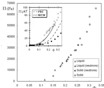
FIG. 2: Equation of state of the silica nanoparticles at I = 10−2mol/L. The filled symbols correspond to the samples studied by SANS and presented in figure 3. Inset: comparison of our exper-imental measured curve (open circles) with the experexper-imental curve measured by Changet al[14] (filled black circles) and with the dif-ferent theoretical modeling of the equation of state proposed in ref [14] (see text).
Macroscopically the transition between fluid and solid samples occurs at low volume fraction atΦT ≈0.23 for an osmotic pressure close to 23000 Pa though it occurs at much larger value for suspensions of hard spheres aroundΦspheresT
≈0.5 [1]. The simplest model that can be imagined [7, 16] to model the threshold transition is to describe the nanoparticles as hard-spheres with an effective radiusR0+δ, sum of their radius and a characteristic range of repulsionsδ. This corre-sponds to an effective renormalized effective volume fraction
Φe f f:
Φe f f=Φ
1+ δ
R0 3
(4) According to the celebrated DLVO theory [23], the typical range of repulsions in our electrostatically stabilized system is the Debye lengthκ−1which value is 31 ˚Afor an ionic strength of 10−2mol/L. A calculation ofΦe f f
T with such a repulsion range gives ≈0.6 which is in the correct range of order of volume fraction for the transition.
[22]. Our system is indeed well described by an MCM model calculation on exactly the same system proposed by Changet alin Ref [14] since our experimentally measured equation of state nicely matches their calculation (see inset of Figure 2).
B. Structure factors of samples made with the standard osmotic stress method
We present in figure 3.a the structure factors of all the sam-ples forming the equation of state of figure 2 in the region of the phase diagram located close toΦT.
FIG. 3: Structure factors of samples in the vicinity of the fluid-solid transition. (a) : structure factors; inset : zoom on the q-range of the correlation peak; (b) low q regime and determination ofκT; (c)
Check of the homogeneous distribution of the centers of mass of nanoparticles within the samples.
It appears at first sight that all these structure factors have the characteristics features of repulsive fluid systems: They have a very small intensity at low q that increases up to a strongly marked correlation peak at q* in the interme-diate q-range, corresponding to the most probable distance between nanoparticles, followed by its harmonics, and ul-timately tends towards 1 at large q. None of the samples presents the Bragg peaks one would have obtained in col-loidal crystals. The solid samples are thus glassy. Even if the polydispersity of the suspension is negligible, the system has not crystallized in the solid part of the phase diagram. In the low q regime, one probes the fluctuations of density at large scale. Since the scattering is very low in this region, there are absolutely no aggregates in the system. When q tends towards 0,S(q)q→0tends towardsΦkTκT whereκT = (δΠ)/(δΦ)−T1is the isothermal compressibility of the system. Inset of figure 3.b shows thatS(q)q→0and thusκT decrease when increases
Π, proving that the system becomes more and more
repul-sive when the osmotic pressure is increased. Nicely, figure 3.b shows that 1/S(q)q→0, a parameter directly measured on
the nanoparticles, is linear withΠ/Φ, a parameter extracted from the PEG20000concentration, showing that the osmotic pressure of the polymer solution is indeed transferred to the suspension of nanoparticles.
Since the system is repulsive, the centers of mass of nanoparticles in the fluid samples should be spatially homo-geneously distributed whatever the samples. This can be eas-ily checked with the position of the correlation peak q* that provides a mean distance between particles ofdmean(2π/q*). If the nanoparticles are homogeneously dispersed, the mean distance between nanoparticles would be varying withΦlike:
dmean= (2R0)( π 6Φ)
1/3 (5)
This hypothesis is checked in Figure 3.c forΦ≤ΦT that proves thatd3meanis linear with 1/Φ. The slope of the curve enables to recover the radius of the nanoparticles. We get here R0= 73±5 ˚A, in accordance with the radius obtained from the form factor measurement.
The shape and the value of the maximum of the intensity of the correlation peak Smax provide an insight of the local order of the organization of the system. The more marked the correlation peak, the better the organization of the sys-tem. One expects thus thatSmaxwould progressively increase with an enhancement of the electrostatic repulsions, that de-creasesκT, provoked by an increase of the osmotic pressure. This is true as long as the samples remain fluid with a volume fraction far lower fromΦT. ButSmaxdecays with an increase ofΦwhen approachingΦT. This decay is compensated by a widening of the correlation peak. This is particularly visible for the two glassy solid samples whom second order peak is also strongly affected. This suggests that the system is less or-ganized in the glass state that in the fluid one. This shows that the system has not explored all the space of phases available to get its optimal configuration due to the vitreous transition. It is particularly striking that the fluid samples just belowΦT start to be affected by freezing, in accordance to the slowing of dynamics observed close to the glass transition of colloids [17, 25].
C. Crossing the fluid-solid transition by small jumps of osmotic pressure
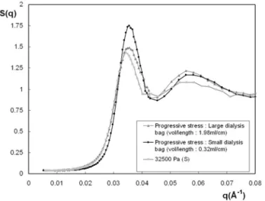
compared with one of the samples already shown in figure 3, prepared with the standard procedure for osmotic stress, that has a close osmotic pressure. It appears that the two sam-ples are glassy. Even with the procedure we use, the jump of pressure of 1000 Pa from one bath to another was too high to allow crystallization. But the way of preparation has clearly an impact. The samples prepared with the progressive stress are better organized than with the standard procedure: the correlation peak and the second maximum are more marked in case of the progressive stress. This is particularly true for the sample prepared by progressive stress with the smallest vol/length: itsSmax has a value of≈1.8 though it is around 1.4 for the sample prepared in the same bag with the standard procedure. For the sample with the larger vol/length, Smax is slightly higher (≈1.5) than for the sample made with the standard procedure. Reciprocally, the decay of the structure factor towards q = 0 in the low q region is sharper for the sam-ple prepared with the progressive stress. This experiment also proves that the specific surface of the bag has a huge influence on the final structure. The system is indeed much better orga-nized when the surface exchange with the reservoir is favored (compare the correlation peak of the sample in small and large dialysis bags in Figure 4). This suggests that there may have spatial heterogeneities of structure, at the macroscopic scale, in the sample made in the large bag.
FIG. 4: Structure factor of samples that have crossed the fluid-solid transition by small jumps of osmotic pressure for different dialysis bags (see text), compared with a sample made with the standard pro-cedure.
This experiment definitely proves that the system can ex-plore more efficiently the space of states if it is let during a rather long time close to the fluid-solid transition and if it has a large surface of exchange with the reservoir. It is likely that a progressive compression which smaller jumps of osmotic pressure such as 100 Pa enables the formation of a crystal, but such an experiment is very time consuming. On the basis of the conclusion of this experiment, we have thus decided to get a deeper insight on the kinetics of the process of the os-motic pressure and of the spatial homogeneity at macroscopic scale of solid samples after an osmotic stress.
D. Kinetics of evolution of the structure of the system during an osmotic stress experiment close toΦT
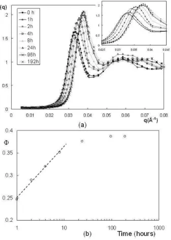
In order to measure the kinetics of an osmotic stress exper-iment we have performed the following experexper-iment: we have prepared a very large reservoir with a given osmotic pressure of 25000 Pa just below the fluid-solid transition. We have prepared 8 dialysis bags with the same amount of nanopar-ticles and placed all the bags in the reservoir. We have then changed the reservoir several times up to the equilibrium. We have then removed one bag and placed all the others in a reser-voir with an osmotic pressure 10000 Pa higher than the initial one (Π= 35000 Pa, t =0). We have then removed the dialysis bags at different times after the start of the pressure jump. It appears that the first samples where rheologically liquid up to 8 hours with an increasing viscosity. At t = 24 hours, the sample was close to the fluid-solid transition and samples at later times were solid. The structure factors obtained at the different times are presented in Figure 5.a. It shows that the structure factor of the sample strongly evolves with time dur-ing compression but keeps the main features observed for the samples at equilibrium time: (i) a strong correlation peak and (ii) a very weak compressibility, proving that the structure of the suspension remains continuously homogeneous during the compression stage. It also clearly appears that the system orders progressively during this compression stage because the intensity of the maximum of the correlation peak Smax increases: It is around 1.6 after 1 hour and increases up to 2.05 after 1 week. Conversely, S(q)q→0 decreases. Figure 5.b shows the evolution of the volume fraction of suspension during the kinetics, as extracted from SANS (see Equ 3). It strongly increases in the first hours of the compression stage and reaches a plateau after 24 hours, showing that the system is close to equilibrium after that time. The increase of the volume fraction as a function of time is linear in a log-linear representation, showing that the volume fraction evolves to-wards a stationary state with an exponential decay time. It enables to extract a characteristic time of≈3 hours. This ki-netics study shows that the evolution of the system is very fast in the early stages of the compression and that the system has reached equilibrium after several days. This is consistent with the procedure usually used in the literature: 3 or 4 changes of baths on a 3 weeks period (our kinetic study was limited to a single change of bath). But it clearly demonstrates that if one wants to compare the characteristic time of a given system with a characteristic time of an osmotic stress experiment, the relevant experimental time of the osmotic stress is the one provided by the kinetic study of the stress (3 hours here) but not the full time of experiment chosen to ensure that equilib-rium is reached (3 weeks usually). At this stage, we can say that the time extracted from our experiment is very probably not universal and that it can be presumably affected by param-eters such as the intensity of the osmotic pressure jump, the initial volume fraction of the suspension, the Debye length...
E. Spatial macroscopic homogeneity of a sample after a strong jump of osmotic pressure close toΦT
FIG. 5: (a) Kinetic evolution of the structure factor of the sample during an osmotic stress experiment; (b) Kinetic evolution of the vol-ume fraction of nanoparticles during an osmotic stress experiment. The dashed line is a guide for the eye.
prepared by the standard procedure≈10ml of suspension in a large dialysis bag (vol/length = 1.98ml/cm) just below the fluid-solid transition at 25000 Pa. We put then sample in a reservoir with a very large osmotic pressure of 220000 Pa (130g/L ofPEG20000!). After one day, the dialysis bag was nevertheless strongly shrunk and has fallen down in the bot-tom of the reservoir. This comes from the fact that a large cohesive solid sample with a high content of silica nanopar-ticles (of density≈2.2 g/cm−3) becomes sensitive to grav-ity. Moreover the bag was larger in the bottom of the reser-voir than in the middle. This gives a rather anisotropic ’pear’ shape to the sample (see inset of figure 6). We still let the sus-pension one week more in the reservoir and removed it from the bag. The sample was strongly solid and was unmoulded with great caution, gently cutting the membrane bag with a knife. The sample was then cut in different parts in order to measure its structure in different spatial regions. 5 parts were tested, as represented in the inset of Fig. 6. The first striking result on this sample concerns its mechanical behav-ior: the texture was not homogeneous. At the border of the sample, it was rock-solid and breakable whereas in the center of the sample it was more jelly-like. The elastic moduli G’ should thus be very different in the different parts of the sam-ple. Please note that G’ is in practice very difficult to measure because the sample dries very fast if it is not kept in a sealed tube. The structure factors derived from SANS confirm that the local structure of the sample differs from one region to
an-other (Figure 6). There are thus density heterogenities within the sample at macroscopic scale. The correlations peaks and compressibilities are very different in the different regions of the sample: The maximum of the correlation peakSmaxhas a higher value in the parts located in the borders of the sample than in the center, respectivelyκT is much lower in the bor-ders than in the center. The system is thus better organized in the borders of the sample in the regions that were close to the dialysis bag than in the regions far from the bag in the center of the sample. Plus, there are small differences in the position of the q* that show that the most probable distance between nanoparticles also slightly differs within the sample.
FIG. 6: Structure factors in the different parts of a large sample ob-tained by a strong jump of osmotic pressure during an osmotic stress pictured in the inset in the upper left.
Since we have shown that the kinetics of compression is fast in the early stages, the following scenario can explain the formation of such spatial heterogeneities. In the early stages of compression, the areas of the sample in contact with the membrane, i.ewhere the exchange of water with the reser-voir occurs by diffusion, are expected to vitrify sooner than the center of the sample. Since the pressure imposed here is very high, the sample becomes very rigid in the vicinity of the membrane, thus forming a continuous shell. The inner part of the sample, which has not reached kinetic equilibrium so far, is now enclosed rigidly by the outer part and thus its relaxation towards kinetic equilibrium is hindered mechani-cally. The outer part of the sample, as it is rigid, keep a con-stant volume to the sample, preventing the compression from going further on and maintaining the inner part at a lower os-motic pressure as if the outer part was a solid container not transmitting the pressure constraint.
This last experiment shows thus that the osmotic stress method forces the sample to have a very heterogeneous glassy structure when the pressure imposed is very high.
IV. CONCLUSION
diagram of a given colloidal system in the region of the high volume fractions, and especially crystalline samples because it does not always allow to reach thermodynamic equilibrium. The technique tends to induce the vitrification of the system, even if the fluid-solid transition is approached by small jumps of pressure. We have indeed not succeeded to get a crys-tal with rather monodisperse silica nanoparticles by jumps of 1000Pa. The kinetics of the osmotic stress process is indeed fast in its early stages as it has an exponential decay time with a characteristic time of a few hours in our experimental con-ditions. Moreover, a strong jump of osmotic pressure during an experiment can freeze the system enough that it becomes macroscopically heterogeneous.
We believe nevertheless that the technique is unequaled to properly prepare colloidal aqueous suspensions with con-trolled physico-chemical parameters. But some rules have to be respected for the preparation of samples with high volume fraction content (crystals, gels, glasses, nematics):
- The parameters that may influence electrostatic interac-tions (pH and salinity) should be first imposed by several stresses at low osmotic pressure in the fluid state; otherwise they may produce an important jump of pressure in the early stages of the stress that may induce irreversible aggregation.
- The dialysis bag should have the lower vol/length possible to increase exchange with reservoir.
- The increase of pressure towards concentrated regions of the diagram should be done by very small jumps of pressure, keeping the bag in the reservoir at least for 24 hours at each step. A further continuation of this work would obviously be to apply these rules on the same systems to try to obtain the crystalline structure observed by Changet al[14]. An other exciting experiment would be to test the influence of the os-motic stress method on the reversibility of the fluid/crystal transition, starting from a colloidal crystal, decaying the os-motic pressure up to the fluid state and coming back to its initial osmotic pressure.
[1] P.N. Pusey, in Liquids, freezing and glass transitions, edited by J.P Hansen, D. levesque, J. Zinn-Justin, (North-Holland, Ams-terdam 765 (2002)).
[2] P.A. Buining, A.P. Philipse, H.N.W. Lekkerkerker, Langmuir,
10, 2106-2114, (1994). P. Davidson, C. Bourgaux, L. Schout-teten, P. Sergot, C. Willams, J. Livage, Journal de Physique II,5(10), 1577-1596, (1995).
[3] F.M. Van der Kooij, H. N. W. Lekkerkerker, J. Phys. Chem. B,102, 7829, (1998). F. M. Van der Kooij, K. Kassapidou, H. N. W. Lekkerkerker, Nature,406, 868, (2000). A.B.D. Brown, S.M. Clarke, A.R. Rennie, Langmuir,14, 3129-3132, (1998). A.B.D. Brown, C. Ferrero, T. Narayanan, A.R. Rennie, Eur. Phys. J. B,11, 481-489, (1999). D. Van der Beek, H. N. W. Lekkerkerker, Europhys. Lett.,61, 702, 2003. D. Van der Beek, H. N. W. Lekkerkerker, Langmuir,20, 8582-8586, (2004). [4] P.A. Forsyth , S. Marcelja, D.J. Mitchell, B.W. Ninham, Adv
Coll Int Sci,9, 37-60, (1978).
[5] G. J. Vroege, H. N. W. Lekkerkerker, Rep. Prog. Phys., 55, 1241, (1992).
[6] S. Hachichu, Y. Kobayashi, A. Kose, J. Coll. Int. Sci,40(2), 342-348, (1973).
[7] P.N. Pusey, W. Van Megen, Nature 320, 340,1986.
[8] E.B Sirota, H.D Ouyang, S.K. Sinha, P.M. Chaikin, J.D. Axe, Y. Fujii, Phys. Rev. Lett.,62(13), 1524-1527 (1989).
[9] Y. Monovoukas, A.P. Gast, J. Coll. Int. Sci, 128, 533-548, (1989).
[10] B. Vincent, J. Edwards, S. Emmett, R. Croot, Colloids and Sur-faces,31, 267-298, (1988).
[11] E. Dubois, R. Perzynski, F. Bou´e, V. Cabuil, Langmuir, 16, 5617-5625, (2000).
[12] F.Cousin, E. Dubois, V.Cabuil, J. Chem. Phys.,115(13), 6051-6057, (2001).
[13] V.A. Parsegian, N. Fuller and R.P. Rand., Proc. Nat. Acad. Sci.,
76(6), 2750, (1979).
[14] J. Chang, P. Lesieur, M. Delsanti, L. Belloni, C. Bonnet-Gonnet, B. Cabane, J. Phys. Chem.,99,15993-16001, (1995). [15] A. Mourchid, A. Delville, J. Lambard, E. Lcolier, P. Levitz,
Langmuir, 11(6), 1942-1950, (1995). P. Levitz, E. Lecolier, A. Mourchid, A. Delville, S. Lyonnard, Europhys. Lett,49(5), 672, (2000).
[16] F.Cousin, E. Dubois., V.Cabuil, Phys. Rev. E, 68, 021405, (2003).
[17] G. M´eriguet, E. Dubois, V. Dupuis, R. Perzynski, J. Phys. Con-dens. Matter,18(45), 10119-10132 (2006).
[18] F.Cousin, V.Cabuil, P.Levitz, Langmuir, 18, 1466-1473, (2002).
[19] C.F. Tejero, A. Daanoun, H.N.W. Lekkerkerker, M. Baus, Phys. Rev. Lett.,73(5)), 752 (1994). C.F. Tejero, A. Daanoun, H.N.W. Lekkerkerker, M. Baus, Phys. Rev. E.,51(1))), 558, (1995).
[20] P. Bartlett, J. Chem. Phys.,107, 188 (1997).
[21] http://www.brocku.ca/researchers/peter rand/osmotic/data/peg20000
[22] C. Bonnet-Gonnet, L. Belloni, B. Cabane, Langmuir,10, 4012-4021 (1994).
[23] B.V. Derjaguin, L. Landau, Acta Physicochim. CCCP,14, 633-662, (1941). E.J.W. Verwey, J.T.G. Overbeek, Theory of the stability of Lyophobic colloids, Elsevier, Amsterdam, (1948).
cited in: J. Israelachvili, Intermolecular and Surface Forces, Academic Press, New York, (1992).
[24] N.F. Carnahan, K.E. Starling, J. Chem. Phys.,51, 635 (1969). [25] A. Robert, E. Wandersman, E. Dubois, V. Dupuis, R.