The Proton Momentum Distribution in Water and Ice
G.F. Reiter,
Physics Department, University of Houston, Houston, Texas, USA
J. C. Li,
Department of Physics, University of Manchester, PO Box 88, M60 1QD, UK
J. Mayers, T. Abdul-Redah,
ISIS Facility, Rutherford -Appleton Laboratory, Chilton, Didcot, OX11 0QX, UK
and P. Platzman,
Lucent Technologies, Murray Hill, New Jersey, USA
Received on 21 October, 2003.
Deep Inelastic Neutron Scattering (Neutron Compton Scattering), is used to measure the momentum distribu-tion of the protons in water from temperatures slightly below freezing to the supercritical phase. The momentum distribution is determined almost entirely by quantum localization effects, and hence is a sensitive probe of the local environment of the proton. The distribution shows dramatic changes as the hydrogen bond network be-comes more disordered. Within a single particle interpretation, the proton moves from an essentially harmonic well in ice to a slightly anharmonic well in room temperature water, to a deeply anharmonic potential in the supercritical phase that is best described by a double well potential with a separation of the wells along the bond axis of about 0.3 Angstrom. Confining the supercritical water in the interstices of a C60powder enhances this
anharmonicity and enhances the localization of the protons. The changes in the distribution are consistent with gas phase formation at the hydrophobic boundaries and inconsistent with the formation of ice there.
1
Introduction
The development of pulsed neutron sources such as ISIS at the Rutherford Laboratory in England have, for the first time, made possible the measurement of proton momentum distributions in solids and liquids. These measurements are analogous to the measurement of electron momentum distri-butions by Compton scattering[1] of light and measurement of nucleon form factors by Deep Inelastic Electron Scatter-ing [2]. The method is known as Neutron Compton Scat-tering (NCS) or Deep Inelastic Neutron ScatScat-tering (DINS). All three techniques rely upon the fact that if the momen-tum transferred from the incident to target particle is suffi-ciently large, the impulse approximation (IA) can be used to interpret the data. In the IA, momentum andkineticenergy are conserved. From a measurement of the momentum and energy change of the neutron, the momentum of the target nucleus before the collision can be determined. The valid-ity of the impulse approximation is due to the fact that as the momentum transfer increases, the characteristic time for the scattering decreases, and the forces on the particle due to its surroundings have less effect, until in the large q limit, the particle behaves as though it is free for the duration of the scattering event [3]. The scattering at these energies is entirely incoherent, each particle scattering independently.
SM(~q, ω), the scattering function for a particle of mass M,
is related to the momentum distribution of the particlen(~p) in this limit by the relation
SM(~q, ω) = Z
n(~p)δ(ω− ~q
2
2M − ~ p.~q
M)d~p (1)
where~ωis the energy transfer, M is the mass of the pro-ton, and q=|~q|is the magnitude of the wave-vector transfer. The small mass of the proton leads to a broad distribution in energy of the scattered neutrons, centered at ~22Mq2, that is
well separated from the scattering from the heavier ions such as oxygen, which appear as nearly elastic contributions[4]. This, together with its large incoherent cross-section, make hydrogen an ideal candidate for these measurements, al-though they are feasible on other light ions as well.
2
Experimental Setup
by a resonance filter difference technique[7]. The water and poly-crystalline ice data were taken in standard aluminum sample holders, 10cm by 10cm by 1mm, thin enough to lead to small multiple scattering, which was in all cases, corrected for. A high pressure cell was designed specif-ically for the high temperature measurements. The back-ground from this ZrTi cell appears as inelastic scattering and is readily subtracted[4]. It can take pressure up to 2000 bar and temperature up to 450oC. The sample size in the
cell is 7 mm in diameter and 30 mm in height. The heaters and temperature sensors were all inserted in the cell. A 1 mm steel pipe leads to an external water-pressurizer (i.e. a pump) which provided the required pressure. The water used as pressure transfer media and the sample volume was distilled H2O.The smaller volume of water in the beam for
the high temperature measurements accounts largely for the poorer statistics. The time scale for the measurements is
10−15−10−16 sec[3], much shorter than the time for the
dissolution of a particular hydrogen bond, so that the mo-mentum distribution we measure can be thought of as re-sulting from a static local structure.
3
Data Analysis
It is clear from Eq. 1 that the measurements do not give directly the momentum distribution, but rather the Radon transform of that distribution. Fortunately, no information is lost from what appears at first sight to be an averaging pro-cedure, and the transform is invertible to obtainn(~p). We representSM(~q, ω)as Mq J(ˆq, y)wherey = Mq (ω−
~q2
2M).
When the sample is either poly-crystalline or a liquid, the average momentum distribution has no angular dependence, andJ(ˆq, y)is independent ofqˆ. It is then straightforward to show thatn(p)can be determined fromJ(y)as
n(p) = −1 2πy
δJ(y)
δy |y=p (2)
We will not use this, but fit the data with a series expansion of the form
J(y) = e
−y2
2σ2 √
2πσ X
n an
22nn!H2n( y
√
2σ) (3)
where theHn(y)are Hermite polynomials.
This series is truncated at some order(2n = 14in this case). The coefficientsanthen determine the measuredn(p)
directly as a series in Laguerre polynomials [4]:
n(p) = e
− p2
2σ2
(√2πσ)3
X
n
an(−1)nL
1 2
n( p
2
2σ2) (4)
A relation between the derivative of Hermite polynomials and Laguerre polynomials[8] ensures that Eq. 2 is satisfied. The procedure is a smoothing operation, which works with noisy data, and which also allows for the inclusion
of small corrections to the impulse approximation[4, 9]. The leading term of the correction has the functional form
H3(y)/q. This is added to the expansion in Eq. 3 with an
undetermined coefficient The entire expression is then con-volved with the instrumental resolution function and fit to the data to determine the coefficients in the expansion. The errors in the measuredn(~p) are determined by the uncer-tainty in the the measured coefficients, through their corre-lation matrix, which is calculated by the fitting program.The uncertainty in the measurement ofn(~p) at some point~pis due to the uncertainty in the measured coefficients. Denot-ing an arbitrary coefficient byρi, we have
δn(~p) =X
i δn(~p)
δρi
δρi (5)
The fitting program, after a minimum is obtained with some set of coefficients, calculates the correlation matrix
< δρiδρj >[10]. Hence, the variance in the momentum
distribution is
< δn(~p)2
>=X
i,j δn(~p)
δρi δn(~p)
δρj
< δρiδρj > (6)
A further refinement is that we set the coefficienta1to zero
in the expansion. This is necessary because the scale fac-tor,σ, in Eq. 3 is undetermined. The expansion is true for any value ofσ. As a consequence, the coefficienta1and the
Gaussian scale factorσin the expansion are strongly corre-lated in the least squares fit, leading to indeterminacy in the fits if botha1andσare varied. Settinga1to zero has the
fur-ther benefit that the total kinetic energy is then determined entirely byσ, even for strongly anharmonic momentum dis-tributions [11]. In units in which σ is measured in ˚A−1,
and the energy is expressed in milli-electron volts, the total kinetic energy(for a proton) is K.E.=6.2705σ2
.
4
Experimental Results
When fit in the way described above, which we will call a free fit,[10] since there is no model assumed, we find that in fact there are at most two coefficients that are statistically significant,a2anda3, for all the data except the room
tem-perature water, wherea5anda6are significant(barely). We
will consider room temperature water in more detail below. In order to make clear that the changes we see are not due to differences in the fitting functions used, we will present the results for all the fits with onlya2anda3included in the
Table 1. Parameters for Free Fit
Water Sample σ(A˚−1) a4 a6
Ice -4C 4.579 0.060±0.0014 −0.068±0.016
Water 23C 4.841 0.185±0.012 0.015±0.015
T=400C, P=750bar 6.363 0.271±.022 0.157±0.028
T=400C, P=750bar in C60 6.439 0.592±0.054 0.007±0.07
The values ofσare not given error bars because in the final fit, they are taken as scale parameters.
5
Interpretation of the Data
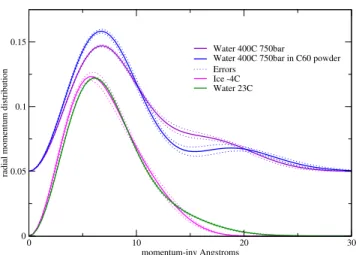
This representation should be regarded as the data forn(p)
determined by the measurement. We show in Fig. 1 a com-parison of the free fits to the data for ice, water at room tem-perature, supercritical water, and supercritical water con-tained in the interstices of a C60 powder. The typical size
for the interstices is 100 ˚A. The quantity4πp2
n(p), the ra-dial momentum distribution is presented, in order to com-pare quantities with the same normalization.
0 10 20 30
momentum-inv Angstroms 0
0.05 0.1 0.15
radial momentum distribution
Water 400C 750bar
Water 400C 750bar in C60 powder Errors
Ice -4C Water 23C
Proton Momentum Distribution in Water and Ice
Figure 1. Comparison of fits to the data of the radial momentum distribution, 4πp2
n(p) for a range of conditions from ice to su-percritical water, to susu-percritical water in the interstices of a C60
poly-crystalline powder, corresponding to increasing disorder in the hydrogen bond network. The 400oC data has been shifted up for clarity.
The kinetic energy due to the temperature has a small ef-fect on the momentum distribution. Even at the highest tem-perature, the thermal kinetic energy corresponds to a mo-mentum width of only about 3 ˚A−1. The corrections to the
momentum widths for the ice due to the finite temperature, are negligible along the bond and only a few percent trans-verse to the bond. What we are seeing is nearly entirely a quantum effect, reflecting the local structure of the proton environment. The structural changes in going from ice to water are noticeable in the data. The tail of the distribution is due to the momentum along the bond direction, since the proton is most tightly bound in this direction, and it is clear
that this width has increased. The shift to a higher momen-tum width along the bond axis can be interpreted as due to the slight increase in the average hydrogen bond distance, so that the proton becomes more tightly bound to its covalently bonded oxygen. The change in the covalent bond length is only about 4% but the measurements are clearly accurate enough to see this shift. This interpretation can also be ap-plied to the supercritical water data, where the density is only 0.65 gr/cc, explaining the greatly increased momentum width. However, the second peak in that data, is entirely un-expected from this simple picture of the bond. One could try to interpret the second peak as a small population of pro-tons with unusually high momentum. However, this would mean an rms energy of these protons of approximately 2.5 eV, and a localization length of about 0.05 Angstrom. We know of no mechanism for producing such energetic pro-tons, and will not consider this possibility further. We will interpret the data in terms of a single particle in an effective potential due to its neighbors. With this interpretation, the second peak indicates that the proton is coherent over two separated sites along the bond. This can be made clear by fitting the data phenomenologically.
To a first approximation, since the proton is surrounded by much heavier oxygen atoms, the proton momentum dis-tribution can be thought of as arising from its confinement in the potential well provided by the oxygens[12], which can be regarded as fixed in position. The interaction with other protons will modify this potential well. While their effect cannot be truly regarded as arising from a static potential, we will assume, in the spirit of a mean field approximation, that they provide an effective potential for the protons. We can then calculate the momentum distribution as though we had a single particle in a fixed effective potential. In fact, we will define the effective potential as the one that produces the observed momentum distribution when interpreted this way.
We will assume a model, in which, in a frame of refer-ence in which an individual bond is taken to lie along the z axis, the motion transverse to the bond is harmonic and along the bond given by a wavefunction that corresponds in real space to two Gaussians separated by a distanced. We will also assumeσx=σy. We have done fits with this
con-dition relaxed, and find that it is well satisfied. The parame-terσzgives the width of the Gaussians in real space through
anisotropic Gaussian momentum distribution.
n(px, py, pz) =
2cos2
(pzd
2~)
1 +e− d2σz2 2~2
Y
i e−
p2i
2σi2
(2πσi)
1 2
(7)
This Gaussian distribution is then averaged over all angles, the corresponding J(y)fit to the data, and the parameters of the model determined. It is the case that an anisotropic Gaussian, when spherically averaged, is not Gaussian, but has an expansion in the form of Eq. 3, in which σ2
= (2σx2+σz2)/3and the anharmonic terms are determined by
the difference between the momentum widths parallel and perpendicular to the bond[13].
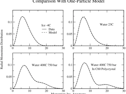
We show in Fig. 2 the fits to that model, and in Table 1 the parameters obtained for those fits. The ice data is very accurately described by an anisotropic Gaussian. The pa-rameters of the Gaussian correspond to vibrational energies in the transverse and longitudinal directions of 105 meV and 332 meV respectively. The water data is also well described this way, with a higher stretch frequency of367 meV and no change in the transverse frequency, although there are clearly additional anharmonicities that make small
correc-tions that are visible in the figure. These may be due to a variation of the effective potential from site to site in the water. Indeed, if the distribution were due entirely to a rota-tionally averaged gaussian, the coefficient ofa3would have
to be negative, and it is not[13]. It may be due as well, how-ever, to an intrinsic anharmonicity in a single bond, perhaps the precursor to the strong anharmonicity seen in the su-percritical water data. Li et al[14] have measured the fre-quency of vibration for hydrogen impurities in D2O ice,
which should be comparable to the frequencies we infer from the anisotropic harmonic fit to our data. They find that the two transverse vibrations are at 105 meV and 200 meV, with the stretch mode at 405 meV. The additional contribu-tions to the anharmonic coefficients may be responsible for the discrepancy with Li et al’s results, since the difference in the transverse mode frequencies we obtain by fitting is very sensitive to the value ofa3.
The fits to the supercritical data require non zero values for the parameter d giving the separation of minima in the potential wells. That is the proton is coherent over sites sep-arated by a distance of approximately 0.3 Angstrom that are both local minima of the potential.
Table 2. Parameters for Model Fit
Water Sample σz(A˚−1) σx(A˚−1) d ( ˚A)
Ice -4C 6.29±0.51 3.53±0.31 0 Water 23C 6.73±0.08 3.51±0.04 0 T=400C, P=750bar 8.40±0.19 5.70±0.16 0.316±0.0045
T=400C, P=750bar in C60 9.47±0.26 5.025±0.11 0.274±0.0043
Momentum-Inv. Angstroms
Radial Momentum Distribution
Comparison With One-Particle Model
0 10 20 30
0 0.05 0.1
Data Model
0 10 20 30
0 0.05 0.1
0 10 20 30
0 0.05 0.1
0 10 20 30
0 0.05 0.1
Ice -4C Water 23C
Water 400C 750 bar Water 400C 750 bar In C60 Polycrystal
Figure 2. Comparison of radial momentum distribution, 4πp2
We know of no prediction of such an effect. The dis-order in the hydrogen bond network would lead to bifur-cated bonds, double bonds, bent bonds and missing bonds. It would seem that these would lead to tunnelling motions transverse to the bond. In our experiment, however, the tun-nelling, or more precisely, the coherence, shows up along the axis with a high momentum width, which is surely the axis of stretching of the covalent bond. To the extent that there are linear bonds, this would be the bond axis. In fact, it is reasonable to think that the supercritical water is made up of small clusters that combine and break up on a time scale much longer than our observation time, so we are see-ing a snapshot average of the ground states for the proton in these small clusters. It is possible then, that what we are seeing is the effect of cooperative tunnelling between bifur-cated bonds and single bonds, as observed in trimers and small clusters [15]. Although the cooperative tunneling mo-tion in these small clusters involves primarily the transverse motion, this could be accompanied by changes in the length of the covalent bond, which is what we see. It is also the case that the temperature is higher than the tunnel splitting in small clusters[15] so we would not expect to see the trans-verse coherence even if the interference it produces occurred at a sufficiently small momentum as to be observable.
The wells are sufficiently separated that the wave-function actually becomes bimodal. We show in Fig. 3 the probability, (the wave-function squared) corresponding to the fitted momentum distributions for the four measure-ments, together with the potential that would produce that wavefunction.
-0.4 -0.2 0 0.2 0.4
Angstroms 0
500 1000
Energy-meV
Probability
23C
400C in C60 polycrystal 400C
Effective Potential and Proton Probability Distribution
Figure 3. Comparison of probability, based on an effective sin-gle particle model, for finding proton at a position along the bond. The zero position is unknown from our experiments, so that the coordinate is relative to the most probable position. The ice and room temperature results are Gaussian, corresponding to harmonic wells. The high temperature wavefunctions are assumed to be the sum of two Gaussians separated by some distance (Table 2), and the potential is that which would produce those wavefunctions.
We note that the interpretation in terms of a single
par-ticle effective potential, although it describes the data well, is not entirely consistent. The tunnel splitting in the two high temperature effective potentials is about 35 meV. With the temperature approximately 70 meV, the two lowest lev-els would be nearly equally populated, and the coherence in the ground state would not be observable. The effective po-tential is then only a phenomenological representation of a more complex many-body phenomenon.
For the water in the interstices of the powdered C60, one
can expect that the the hydrogen bond network will be even more distorted than in the pure water, and we will be seeing an average over bonds that are near the surface with those that are relatively “in the bulk”. The size of the surface layer at ordinary temperatures is in some dispute[16, 17], ranging from 1.5-5nm and it seems certain that it would be signif-icantly larger for the supercritical water. It is conceivable, given the size of the interstices in the C60poly-crystal, that
the entire volume of water would be strongly affected by the contact with the surfaces. Consistent with this, we find that the protons are more localized in the C60 interstices than
in the “free” supercritical water, with both the width of the individual Gaussians in the spatial wave function and their separation decreasing when the water is contained in the C60
interstices.
There is no sign of ice formation at the surfaces. This might be regarded as not terribly surprising, given the tem-perature, but the bond energies involved are still large com-pared to the temperature, and it is conceivable that the pres-ence of the repulsive surface would be sufficient to cause the ice phase to form. We would expect then to see a nar-rowing, rather than a broadening, of the distribution. In any case, the results are consistent with the formation of the gas phase there. Indeed the kinetic energy for the supercritical water(25±6meV is slightly greater than that calculated for the free water molecule (214 meV) at the same temperature and pressure [18].
As is clear from Fig. 2, the room temperature water data is not fit perfectly by the anisotropic Gaussian model. We show in Table 3 a more refined fit of the data with coeffi-cients up toa6included, compared with the prediction from
give accurate results for supercritical water. At low tem-peratures, when the potential is harmonic, the centroid of the proton wavefunction is all that is needed to describe the motion. That can be done classically, as there is no distor-tion of the shape of the Gaussian wave packet as the proton moves. However, the strong anharmonicity present in the effective potential at high temperatures, whatever its origin, would couple the centroid motion with changes in the shape of the wave function, an effect that can not be included in a classical calculation.
Table 3. Comparison of an extended fit of the data for room tem-perature water with those derived from a rotationally averaged anisotropic Gaussian model.
Coefficient Water Data23oC Model Prediction σ 4.848 ˚A−1 4.827 ˚A−1 a2 0.205±0.020 0.168
a3 0.053±0.045 -0.044
a4 0 -0.061
a5 −0.099±0.093 -0.034
a6 −0.094±0.078 -0.032
6
Conclusions
In conclusion, the results shown here, in addition to provid-ing a detailed picture of the dynamics of the proton in water, show that the momentum distribution of the proton, which is sensitive to the local structure of the proton, can be mea-sured with sufficient accuracy to provide detailed informa-tion about that structure, even in liquids or powder samples.
Acknowledgements
One of us (G.R.) would like to thank Tony Haymet and Ariel Chialvo for useful discussions.
References
[1] P. M. Platzmann inMomentum Distributions, ed R. N. Silver and P. E. Sokol (Plenum Press, New York, 1989, p249).
[2] I. Sick in ref 1, page 175.
[3] R. Silver and G. Reiter, Phys. Rev. Letts.54, 1047 (1985).
[4] G. Reiter, J. Mayers, and J. Noreland, Phys. Rev. B 65, 104305 (2002).
[5] P. M. Platzmann, inMomentum Distributions,ed R. N. Silver and P. E. Sokol (Plenum Press, New York, 1989, p249).
[6] J. Mayers and A. C. Evans, Rutherford Appleton Laboratory Report No. RAL-TR-96-044,1996(unpublished).
[7] P. A. Seeger, A. D. Taylor, and R. M. Brugger Nuc. Inst. Meth. A240, 98 (1985).
[8] M. Abramowitz and I. Stegun, NBS Applied Mathematics Series55, P779, (1964).
[9] V. F. Sears, Phys. Rev.185, 200 (1969); Phys. Rev. A7, 340 (1973).
[10] D. Sivia, Data Analysis: A Bayesian Tutorial, Clarendon Press, Oxford (1996).
[11] By definition the kinetic energy isR 2pM2n(~p)d~p. Represent-ingp2
as−L 1 2
1 + 3
2, using Eq. 4 forn(p), and observing that
the Laguerre polynomials are orthogonal with the weighting
in that equation, we obtain K.E.= 3 2Mσ
2
whenL12
1 is omitted
from the sum in Eq. 4.
[12] M. Warner, S. W. Lovesey, and J. Smith, Z. Phys. B39, 2022 (1989).
[13] The average may be done analytically. For the case that the two transverse directions have the same variance, we find
< J(y) >is of the form given in Eq.3, with a1 = 0, σ2
= (2σ2
x+σ2
z)/3, andan=(δσ 2 σ2)
n<(1/3 −cos
2
(θ))n>, where δσ2
= (σ2
x−σ
2
z). Explicitly, a2=4/45(δσ
2 σ2)
2
and
a3= 16/945(δσ
2 σ2)
3
.
[14] J. C. Li, J. Chem. Phys.105, 6733, (2003).
[15] F. N. Keutsch and R. J. Saykally, Proc. Nat. Acad. Sci.98, 10533 (2001).
[16] T. R. Jensenet al., Phys. Rev. Lett.90, 86101 (2003).
[17] R. Steitzet al., Langmuir,19, 2409 (2003).