A comparative analysis of preprocessing
techniques of cardiac event series for
the study of heart rhythm variability
using simulated signals
Laboratório de Hipertensão, Departamento de Fisiologia e Biofísica, Instituto de Ciências Biológicas, Universidade Federal de Minas Gerais, Belo Horizonte, MG, Brasil
H.N. Guimarães and R.A.S. Santos
Abstract
In the present study, using noise-free simulated signals, we performed a comparative examination of several preprocessing techniques that are used to transform the cardiac event series in a regularly sampled time series, appropriate for spectral analysis of heart rhythm variabil-ity (HRV). First, a group of noise-free simulated point event series, which represents a time series of heartbeats, was generated by an integral pulse frequency modulation model. In order to evaluate the performance of the preprocessing methods, the differences between the spectra of the preprocessed simulated signals and the true spectrum (spectrum of the model input modulating signals) were surveyed by visual analysis and by contrasting merit indices. It is desired that estimated spectra match the true spectrum as close as possible, show-ing a minimum of harmonic components and other artifacts. The merit indices proposed to quantify these mismatches were the leakage rate, defined as a measure of leakage components (located outside some narrow windows centered at frequencies of model input modulating signals) with respect to the whole spectral components, and the numbers of leakage components with amplitudes greater than 1%, 5% and 10% of the total spectral components. Our data, obtained from a noise-free simulation, indicate that the utilization of heart rate values instead of heart period values in the derivation of signals representa-tive of heart rhythm results in more accurate spectra. Furthermore, our data support the efficiency of the widely used preprocessing technique based on the convolution of inverse interval function values with a rectangular window, and suggest the preprocessing technique based on a cubic polynomial interpolation of inverse interval function values and succeeding spectral analysis as another efficient and fast method for the analysis of HRV signals.
Correspondence
R.A.S. Santos
Departamento de Fisiologia e Biofísica, ICB, UFMG Av. Antônio Carlos, 6627 31270-901 Belo Horizonte, MG Brasil
Fax: 55 (031) 499-2924
Research supported by CNPq, FAPEMIG and PRPq-UFMG. H.N. Guimarães was the recipient of a CNPq fellowship.
Received May 3, 1996 Accepted October 24, 1997
Key words
•Heart rhythm variability
•Heart rate variability
•Spectral analysis
•Data preprocessing
Introduction
Since the initial experiments of Akselrod et al. (1,2), Pomeranz et al. (3) and Pagani et al. (4), who suggested that the spectral anal-ysis of heart rhythm variability (HRV) could be used as a novel and powerful noninvasive tool for indirect assessment of the sympatho-vagal modulating activity of cardiovascular function, the technique has been extensively used, not only in basic research, but also in clinical medicine (5-8). In the frequency do-main, three underlying frequency bands have been defined through the HRV spectrum observation (1-10) and named: a) “high-fre-quency band” or “respiratory sinus arrhyth-mia related band”, which occurs at about the mean breathing frequency of the patient or experimental animal; b) “low-frequency band” or “Mayer wave-like sinus arrhythmia related band”, which occurs at about 0.1 Hz spontaneous vasomotor activity, and c) “very-low-frequency band”, which is the band of less than 0.05-Hz frequencies. Power alter-ations in the high-frequency band have been attributed to changes in cardiac parasympa-thetic activity, whereas in the low-frequency band they have been related to changes in both sympathetic and parasympathetic ac-tivities (1-8). In contrast, the physiological elucidation of the very-low-frequency band power is much less established (8), albeit some researchers have related it to ther-moregulatory activity, to the renangio-tensin system and to other systems that in-volve humoral factors (1,2,9,10).
The analysis of signals in the frequency domain can be performed either by classical techniques, such as Blackman-Tukey’s correlogram and Welch’s periodogram (11) - both based on the fast Fourier transform (FFT) algorithm (12) -, or by autoregressive modern techniques (11). However, the pro-cessing of a series of non-equidistant point events, constituted by successive heartbeats (cardiac event series), and their analysis in the frequency domain are not
straightfor-ward. Spectra can be estimated only from regularly sampled signals (11), although some techniques propose the direct estimation of the spectra of unevenly sampled data (13,14), but these algorithms are computationally cumbersome. Therefore, the cardiac point processes must be first submitted to math-ematical approaches, denoted in this report as preprocessing procedures, to produce a series of equidistantly sampled data suitable for spectral analysis. This implies that differ-ent spectra can be defined by differdiffer-ent forms of preprocessing. Moreover, the signal of HRV can be either heart period or heart rate, defined as the reciprocal values of each other. These signals have the same informative content, but the results obtained from each have shown considerable discrepancies, in-asmuch as the relationship between them is non-linear (15).
spectra) and a well-defined comparison (us-ing merit indices to quantify the mismatches between the estimated spectra and the true spectrum) of the several methods that can be employed in the signal preprocessing for the analysis of HRV.
Methods
Signal simulation
For the evaluation of the performance of the several methods that can be employed in the signal preprocessing for the analysis of HRV, we used as input signals for the pre-processing algorithms three noise-free com-puter-simulated temporal series of heartbeat intervals generated by an IPFM model.
Information embedded in a series of point events will be described by an IPFM model if, and only if, any two consecutive point event occurrence times, t[n] and t[n + 1], are related by the following equation
T m m t dt
t n t n
= +
+
∫
[ ( ) ][ ] [ ]
0 1 1
Eq. 1 where T is the integrator’s threshold value,
m1(t) is the modulating signal, and m0 is a
constant that links the unmodulated point events rate (intrinsic frequency) with the inverse of the integrator’s threshold value by the relation ƒ0 = m0/T (17-21). The IPFM
model can also be seen as a device that integrates its input signal m(t) = m0 + m1(t)
until the integrated value M(t) reaches a fixed threshold value T, at which time the device generates a point event, resets the integrator to zero and initiates a new cycle of integration. The IPFM model was first em-ployed in electrophysiology for the study of the nerve cell impulse generation process (19) and later Hyndman and Mohn (20) sug-gested it as a functional description of the cardiac sinus node electrophysiology. For the sinus node pacemaker cells, the value
M(t) resembles the membrane potential that
rises until the threshold value is reached and causes an action potential to occur. The dia-stolic depolarization contribution is related to the value m0, and the humoral and
auto-nomic neural influences are represented by the value m1(t). Obviously, when m1(t)
in-creases, equivalent to the preponderance of sympathetic influence, the intervals between the point events shorten, contributing to an increase in heart rate.
In the simulation of the heartbeat inter-vals by the IPFM model, the L feasible modu-latory activities that are lumped together in the value m1(t) have been considered as
os-cillatory components and consequently mod-eled by sinusoidal signals,
m t a l f l t
l L
1
1
2
( )= [ ] sin ( [ ] )
=
∑
π Eq. 2where a[l] and ƒ[l] are, respectively, the am-plitude and the frequency of the l-sinusoid (17,18). In the current study, we simulated three time series of 512 data (henceforth referred to as time series #1, #2 and #3), for which the model’s threshold value T was 1.05 s, m0 = 1, and the other parameters were
established in the following fashion: a) m1(t)
= 0.3sin(2π0.16t) for time series #1; b) m1(t)
= 0.3sin(2π0.12t) + 0.3sin(2π0.16t) for time series #2, and c) m1(t) = 0.3sin(2π0.07t) +
0.3sin(2π0.16t) + 0.3sin(2π0.28t) for time series #3. The parameters used in the forma-tion of the time series #1 and #2 were chosen to carry out the same simulations previously reported by De-Boer et al. (16,17) and Berger et al. (18). In addition, we simulated a third time series, in which the modulating signal was comprised of three oscillatory compo-nents with frequencies equal to 0.07, 0.16 and 0.28 Hz. The values of T = 1.05 s and
m0 = 1 imply, by definition, an intrinsic
results in heartbeat intervals whose length is up to approximately 30% different from the mean value.
Signal preprocessing
The term preprocessing is employed in the current report to designate the math-ematical approaches used in the derivation of an equidistantly sampled time series from irregularly sampled cardiac event series. The several spectra that were studied in this re-port (listed in Table 1) are defined below.
The spectrum of heart periods (or spec-trum of intervals) is the specspec-trum of the interval tachogram, which is defined as the series of heartbeat intervals as a function of interval number (9,16-18,22,23). In this man-ner, the intervals can be visualized as regu-larly spaced, but, as a consequence, the units of the frequency axis of these spectra are “cycles per beats” rather than “Hertz”. In a different way, if the intervals should be con-sidered evenly spaced with distances equal
to the average interval length, the frequency unit will be “cycles per second” or “Hertz equivalent”. This method has been exten-sively used (4-8) since it was first suggested by Sayers (9).
Additionally, a large class of spectra arises from a spectral estimation of the series ob-tained by a regular sampling of sectionally continuous functions derived from the car-diac event series. We labeled this class as
spectrum of sampled sectionally continuous interval function. For the determination of these functions, numerous possibilities ex-ist, and in the current study we used the following ones: a) The function values are maintained constant from the time of occur-rence of the nth cardiac event, t[n], to the time of occurrence of the succeeding one,
t[n + 1], and this constant value can be the instantaneous heart period (ƒ(t) = t[n + 1]
-t[n] for t[n] ≤t < t[n + 1]) or the delayed heart period (ƒ(t) = t[n] - t[n - 1] for t[n] ≤ t <
t[n + 1]). These sectionally continuous inter-val functions are known as instantaneous heart period signal and delayed heart period signal, respectively (21). b) The function val-ues are determined through the convolution of the instantaneous heart period signal with a rectangular window of width equal to twice the sampling period of the posterior sam-pling procedure, divided by the window width. It is important to note that the convo-lution of a signal with a rectangular window in the time domain corresponds, in the fre-quency domain, to the multiplication of the Fourier transform of this signal with a low-pass filter with a transfer function equal to
H f f T
f
w
( )= sin (π )
π Eq. 3
where Tw is the window width (12).
Conse-quently, when this type of preprocessing technique is used, the power spectrum esti-mate can be improved if multiplied by the correction factor [Tw/H(ƒ)]2. Furthermore,
the spectral estimate can be considered ac-curate only for 0<ƒ<ƒs/4, where ƒs is the
Table 1 - Spectrum types of heart rhythm variability derived from the various prepro-cessing techniques used to transform the cardiac event series into a regularly sampled time series.
Spectrum Description
Cluster 1: spectra derived from the heart periods
#1 spectrum of heart period (spectrum of intervals) #2 spectrum of sampled delayed heart period signal #3 spectrum of sampled instantaneous heart period signal
#4 spectrum of sampled function of linear-interpolated heart period values #5 spectrum of sampled function of cubic-interpolated heart period values #6 spectrum of sampled function of 5-degree-interpolated heart period values #7 spectrum of sampled instantaneous heart period signal convoluted with
a rectangular window
Cluster 2: spectra derived from the heart rate
#8 spectrum of heart rate (spectrum of inverse intervals) #9 spectrum of sampled delayed heart rate signal #10 spectrum of sampled instantaneous heart rate signal
#11 spectrum of sampled function of linear-interpolated heart rate values #12 spectrum of sampled function of cubic-interpolated heart rate values #13 spectrum of sampled function of 5-degree-interpolated heart rate values #14 spectrum of sampled instantaneous heart rate signal convoluted with
a rectangular window
sampling frequency. This method was sug-gested by Berger et al. (18), who used the instantaneous heart rate signal instead of the instantaneous heart period signal as described here. c) The function values are determined by means of some kind of interpolation of the interval function values. The interval function is defined as the series of heartbeat intervals as a function of time, in which impulses are formed only at the event occur-rence times with an amplitude equal to the length of the preceding interval (23,24). In the current study, we employed the efficient Neville’s algorithm for evaluation of poly-nomial interpolations (13).
Finally, another spectrum can be assessed in a straightforward manner from the non-equidistant cardiac event series in which the series of cardiac events was replaced with a train of impulse functions (Dirac’s delta func-tions),
p t
t t n
n N
( )
=
(
[ ])
=
∑
δ
-0 1
Eq. 4
where N is the number of cardiac events and
t[n] (n∈ N; 0 ≤n≤N - 1) is the occurrence time of the nth event. This power spectrum, known as spectrum of counts (14,16-18,25), is defined as the low-frequency part of the squared Fourier transform of the sequence of impulse functions p(t), and can be analyti-cally calculated as
+ − = ∑ = 2 1 -0
2 cos(2 [ ])
] 1 -[ 2 ) ] 1 -[ 2 ( sin ] 1 -[ ) ( N n n t f N t f N t f N N N t f P π π π +∑ = 2 1 -0 ) ] [ 2 ( sin ] 1 -[ 2 ) 1 -) ] 1 -[ 2 ( cos ( N n n t f N t f N t f N π π π Eq. 5
As pointed out by Berger et al. (18), equation 5 embodies terms that compensate for the truncation effects that are brought about by the computation of the Fourier transform of a finite set of impulse functions.
With the exception of the spectrum of counts, a further set of spectra can be ob-tained in the same manner as those defined
above if reciprocals of intervals (heart rates) are considered instead of intervals (heart periods).
Signal processing
In the processing of equidistantly sam-pled time series resulting from the prepro-cessing procedures, the spectra were com-puted by means of a windowed FFT algo-rithm (11,12,26), except for the spectrum of counts which was calculated using equation 5. For the sake of comparison with the previ-ous works of De-Boer et al. (16,17) and Berger et al. (18), the amplitude spectrum (the square root of the power spectrum) was adopted. This method has been extensively used to accentuate the presence of harmon-ics and other artifacts, which is helpful in the evaluation of the performance of the spectra (16-18).
Performance evaluation
In an attempt to evaluate the various esti-mated spectrum performances mentioned in Table 1, their shapes were compared to that of the spectrum of the IPFM model modulat-ing signal (true spectrum), responsible for the generation of the simulated heartbeat interval series. These comparisons can be made both by visual analysis (16-18), in which we look for the presence of harmonic peaks and other artifacts in the estimated spectra, or by contrasting merit indices, de-signed for evaluating the performance. As previously noted, it is desired that estimated spectra match the true spectrum as closely as possible and therefore the merit indices used in this study were empirically designed in order to quantify these mismatches. In this study, we proposed the following indices: a) the foremost, named leakage rate (SL), is
compo-maining spectrum. b) The numbers of leak-age spectral components with amplitudes greater than 1% (n1%), 5% (n5%) and 10%
(n10%) of the total spectral components.
Results
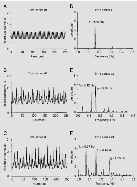
Figure 1A-C shows the interval tacho-grams of the first 250 (of 512) simulated values of time series #1, #2 and #3, respec-tively. These graphs illustrate the increased irregularity (complexity) in the output signal of an IPFM model when more than one modulatory element are lumped together to compound the input model signal. It is a highly laborious task to analyze the nature of the modulating signals only by simple obser-vation of Figure 1C.
For the spectral analysis of the prepro-cessed signals, some commonly used time windows (Bartlett, Hanning, Hamming and Blackman) (26) were first tested and we utilized the Blackman window since this invariably produced the least leakage rate in amplitude spectra.
Figure 1D-F shows the amplitude spectra estimated from the time series #1, #2 and #3, respectively, preprocessed by means of a polynomial cubic interpolation (spectrum of sampled function of cubic-interpolated heart period values). The spectrum shown in Fig-ure 1D contains, in addition to a peak related to modulatory frequency (0.16 Hz), a sec-ond and third harmonic peak (0.32 Hz and 0.48 Hz, respectively). The spectra of Figure 1E and 1F embody peaks at sum and differ-ence frequencies of the model’s modulating frequencies. In Figure 1E, which shows the spectrum related to the signal composed by the modulating frequencies ƒ1 = 0.12 Hz and ƒ2 = 0.16 Hz, the main artifactual peaks are
0.4 Hz (ƒ2 - ƒ1), 0.24 Hz (2ƒ1), 0.28 Hz (ƒ1 + ƒ2) and 0.32 Hz (2ƒ2). In the spectrum of
Figure 1F, the most salient artifactual peaks are 0.02 Hz (ƒ2 - 2ƒ1), 0.09 Hz (ƒ2 - ƒ1),
0.12 Hz (ƒ3 - ƒ2), 0.14 Hz (2ƒ1), 0.21 Hz
(3ƒ1), 0.23 Hz (ƒ1 + ƒ2), 0.30 Hz (2ƒ1 + ƒ2),
Heartbeat interval (s)
3
A
Time series #1
2
1
0
Heartbeat interval (s)
3
B
2
1
0
Time series #2
Heartbeat interval (s)
3
C
2
1
0
Time series #3
Amplitude
8
D
6
4
0
Time series #1
2
Amplitude
8
E
6
4
0
Time series #2
2
Amplitude
8
F
6
4
0
Time series #3
2 0 50 100 150 200 250
Heartbeat
0.0 0.1 0.2 0.3 0.4 0.5 Frequency (Hz)
0 50 100 150 200 250 Heartbeat
0.0 0.1 0.2 0.3 0.4 0.5 Frequency (Hz)
0 50 100 150 200 250 Heartbeat
0.0 0.1 0.2 0.3 0.4 0.5 Frequency (Hz)
f = 0.16 Hz
f1 = 0.12 Hz
f2 = 0.16 Hz
f1 = 0.07 Hz
f2 = 0.16 Hz
f3 = 0.28 Hz
Figure 1 - A, B, C, Interval tachograms of the first 250 (of 512) values of three noise-free simulated time series produced by means of an IPFM model in which the threshold value was 1.05 s and the input signals consisted of a summation of modulating sinusoids with frequencies equal to 0.16 Hz (A), 0.12 and 0.16 Hz (B), and 0.07, 0.16 and 0.28 Hz (C). D, E, F, Amplitude spectra estimated from the three simulated time series preprocessed by means of a polynomial cubic interpolation (spectrum of sampled function of cubic-interpo-lated heart period values).
nents are those located outside some narrow windows (spectrum signal bands) centered at frequencies of IPFM model modulating signals. We have experimentally determined that a width of 12 ∆ƒ (where ∆ƒ = ƒs/N) for
re-0.32 Hz (2ƒ2), 0.35 Hz (ƒ1 + ƒ3), 0.37 Hz
(3ƒ1 + ƒ2) and 0.44 Hz (ƒ2 + ƒ3), where the
modulating frequencies are ƒ1 = 0.07 Hz, ƒ2
= 0.16 Hz and ƒ3 = 0.28 Hz. As can be seen,
besides interval tachograms, the intricacy of spectra markedly increases with the number of modulatory elements at the model input.
For the present analysis, the 15 types of amplitude spectra grouped in Table 1 were divided into three clusters, as follow: a) cluster 1 aggregated the set of spectra derived from the intervals (heart periods), which are spec-tra #1 to #7, b) cluster 2 aggregated the set of spectra derived from the reciprocals of inter-vals (heart rates), which are spectra #8 to #14, and c) cluster 3 consisted of the spec-trum of counts (specspec-trum #15).
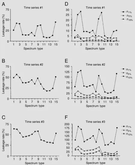
Figure 2A-C presents the computed leak-age rate of the spectra estimated from the time series #1, #2 and #3, respectively, while Figure 2D-F exhibits the numbers of leakage spectral components (n1%, n5% and n10%).
Figure 2A shows that, for the time series #1 and cluster 1, spectra #5, #6 and #4 presented the lowest leakage rates (13.97%, 14.39% and 14.84%, respectively), whereas spectra #2 and #3 presented the highest ones (41.64% and 40.55%, respectively). For clus-ter 2, spectra #12, #13 and #11 presented the lowest leakage rates (8.13%, 8.48% and 9.93%, respectively), whereas spectra #10 and #9 presented the highest ones (37.59% and 35.69%, respectively). Spectrum #15 of group 3 presented a leakage rate of 44.57%. Spectrum #12 presented the lowest leakage rate (8.13%), whereas spectrum #15 pre-sented the highest one (44.57%), implying a variation of 448% between the lowest and the highest leakage rate.
As shown in Figure 2B, for the time series #2 and cluster 1, spectra #5 and #4 presented the lowest leakage rates (36.98% and 37.28%, respectively), whereas spectra #2, #3 and #1 presented the highest ones (56.13%, 49.09% and 48.83%, respectively). For cluster 2, spectra #12 and #13 presented the lowest leakage rates (18.00% and 18.64%,
Leakage rate (%)
75
A
Time series #1
50
25
0
B
C
D
0
Time series #1
E
F
1 3 5 7 9 11 Spectrum type
13 15 30
20
10
1 3 5 7 9 11 13 15 25
15
5
Spectrum type
n1%
n5%
n10%
Leakage rate (%)
75
50
25
0
1 3 5 7 9 11 Spectrum type
13 15
Time series #2 Time series #2
Time series #3 Time series #3
Leakage rate (%)
75
50
25
0
1 3 5 7 9 11 Spectrum type
13 15 0 150
100
50
1 3 5 7 9 11 13 15 125
75
25
Spectrum type
0 200
150
100
1 3 5 7 9 11 13 15 175
125
75
Spectrum type 50
25
Figure 2 - Values of merit indices calculated to assess the performance of the spectra estimated from three noise-free simulated time series. These series were produced by means of an IPFM model in which the threshold value was 1.05 s and the input signals consisted of a summation of modulating sinusoids with frequencies equal to 0.16 Hz (A, D), 0.12 and 0.16 Hz (B, E), and 0.07, 0.16 and 0.28 Hz (C, F). The 15 types of spectra shown here are discriminated in Table 1. A, B, C, Leakage rate. D, E, F, Numbers of leakage spectral components with amplitudes greater than 1% (n1%), 5% (n5%) and 10% (n10%) of the total spectral components.
respectively), whereas spectrum #9 presented the highest one (47.58%). Spectrum #15 pre-sented a leakage rate of 50.55%. Spectrum #12 presented the lowest leakage rate (18.00%), whereas spectrum #2 presented the highest one (56.13%), implying a varia-tion of 212%.
As shown in Figure 2C, for the time series #3 and cluster 1, spectra #4 and #5 presented the lowest leakage rates (44.41% and 45.68%, respectively), whereas spectra
n1%
n5%
n10%
n1%
n5%
#1 and #2 presented the highest ones (63.78% and 62.70%, respectively). For cluster 2, spectra #14, #13 and #12 presented the low-est leakage rates (29.98%, 31.37% and 31.84%, respectively), and spectra #9 and #8 presented the highest ones (58.19% and 57.47%, respectively). Spectrum #15 of group 3 presented a leakage rate of 52.95%. Spectrum #14 presented the lowest leakage rate (29.98%) and spectrum #1 presented the highest one (63.78%), indicating a variation of 113%.
Both the analysis of the numbers of leak-age spectral components n1%, n5% and n10%
(see Figure 2D-F) and the visual examina-tion of the spectrum shapes corroborated the results described above. As evidenced by Figure 2A-F and the analysis reported above, the spectrum of sampled function of cubic-interpolated heart rate values (spectrum #12), the spectrum of sampled function of 5-de-gree-interpolated heart rate values (spectrum #13) and the spectrum of sampled instanta-neous heart rate signals convoluted with a rectangular window (spectrum #14) appear to be the most appropriate for analysis of the HRV signal in the frequency domain.
Discussion
In the present study we compared several methods for the preprocessing of cardiac event series for the analysis of HRV. Our major objective was to extend the studies conducted by De-Boer et al. (16,17) and Berger et al. (18) in two aspects: a) these previous studies only investigated the spec-trum of intervals (16-18), the specspec-trum of inverse intervals (17,18), the spectrum of counts (16-18) and the spectrum of sampled instantaneous heart rate signal convoluted with a rectangular window (18). In the cur-rent study we analyzed a more comprehen-sive group consisting of 15 types of spectra, as described in Table 1. b) In the above mentioned studies the spectra were com-pared only by means of visual contrasting,
while in the current study, besides visual analysis, we performed a well-defined com-parison based on merit indices, designed to quantify the mismatches between the esti-mated spectra and the true spectrum.
The spectrum of intervals - owing to its simplicity - and the spectrum of sampled instantaneous heart rate signal convoluted with a rectangular window - owing to its good performance reported in the study of Berger et al. (18) - are still the most fre-quently employed techniques for the study of HRV signals (1-9). The results obtained in the present study contraindicate the spec-trum of intervals, reinforce the efficiency of the algorithm suggested by Berger et al. (18) and indicate another simple approach which is also efficient for the study of HRV, as discussed below.
We noticed that if the classical methods of spectral estimation are chosen for the analysis of HRV, then the multiplication of the time series with a Blackman window before the signal processing procedures will result in a spectrum with the least leakage rate. In addition, the matched comparison between the spectra of clusters 1 and 2 and their own merit indices indicate a marked decrease in the leakage rate when the heart rates were used instead of the heart period values in the derivation of signals represen-tative of heart rhythm. This result agrees with data reported by Mohn (22), which suggested that the spectrum of inverse inter-vals is superior to the spectrum of interinter-vals. However, the reasons for these discrepan-cies are not clear. The influence of the choice of heart rate or heart period values in the study of HRV has not been sufficiently con-sidered. Only a few recent reports (15,27,28) have speculated this questionable point.
function of cubic-interpolated heart rate val-ues is the most suitable for the study of HRV signals, inasmuch as it more closely matches the true spectrum at the input of the IPFM model when the model’s modulating signal is composed of one or two sinusoidal noise-free signals. Consequently, we conclude that the preprocessing technique based on a cu-bic polynomial interpolation of inverse in-terval function values is an adequate ap-proach for the derivation of an equidistantly sampled time series, representative of the heart rhythm, from the irregular cardiac event series. Furthermore, we observed that the spectrum of sampled function of 5-degree-interpolated heart rate values and the spec-trum of sampled instantaneous heart rate signal convoluted with a rectangular win-dow also closely match the true spectrum, particularly for the case of three sinusoidal noise-free modulating signals. However, from a computational point of view, the assessment of regularly sampled data by means of cubic polynomial interpolation us-ing Neville’s algorithm is the most efficient
and effortless procedure. Conversely, the spectrum of intervals, which is among the techniques most frequently used, is the least effective estimate in the sense that it di-verges considerably from the true spectrum. The results reported here indicate that an accurate and successful spectral estimation is a sine qua non of a carefully selected preprocessing technique. The use of heart rate values instead of the heart period values in the derivation of signals representative of heart rhythm results in more correct spectra. Furthermore, our data derived from math-ematical modeling and noise-free simula-tions reinforce the efficiency of the wide-spread adopted preprocessing technique based on the convolution of inverse interval function values with a rectangular window, and recommend the technique based on a cubic polynomial interpolation of inverse interval function values and succeeding spec-tral analysis as another efficient, fast and more effortless computer implementation set of procedures for the analysis of HRV sig-nals.
References
1. Akselrod S, Gordon D, Ubel FA, Shannon DC, Berger AC & Cohen RJ (1981). Power spectrum analysis of heart rate fluctua-tion: a quantitative probe of beat-to-beat cardiovascular control. Science, 213: 220-222.
2. Akselrod S, Gordon D, Madwed JB, Snidman NC, Shannon DC & Cohen RJ (1985). Hemodynamic regulation: investi-gation by spectral analysis. American Journal of Physiology, 249: H867-H875. 3. Pomeranz B, Macaulay RJB, Caudill MA,
Kutz I, Adam D, Gordon D, Kilborn KM, Barger AC, Shannon DC, Cohen RJ & Benson H (1985). Assessment of auto-nomic function in humans by heart rate spectral analysis. American Journal of Physiology, 248: H151-H153.
4. Pagani M, Lombardi F, Guzzetti S, Rimoldi O, Furlan R, Pizzinelli P, Sandrone G, Malfatto G, Dell’Orto S, Piccaluga E, Turiel M, Baselli G, Cerutti S & Malliani A (1986). Power spectral analysis of heart rate and arterial pressure variabilities as a marker
of sympatho-vagal interaction in man and conscious dog. Circulation Research, 59: 178-193.
5. Malliani A, Pagani M, Lombardi F & Cerutti S (1991). Cardiovascular neural regulation explored in the frequency domain. Circu-lation, 84: 482-492.
6. Van-Ravenswaaij-Arts CMA, Kollée LAA, Hopman JCW, Stoelinga GBA & Van-Geijn HP (1993). Heart rate variability. Annals of Internal Medicine, 118: 436-447. 7. Malik M & Camm AJ (Editors) (1995).
Heart Rate Variability. Futura Publishing Company, Armonk, New York.
8. Task Force of the European Society of Cardiology and the North American Soci-ety of Pacing and Electrophysiology (1996). Heart rate variability - standards of measurement, physiological interpreta-tion and clinical use. Circulainterpreta-tion, 93: 1043-1065.
9. Sayers BMcA (1973). Analysis of heart rate variability. Ergonomics, 16: 17-32. 10. Kitney RI (1987). Beat-by-beat
interrela-tionships between heart rate, blood pres-sure, and respiration. In: Kitney RI & Rompelman O (Editors), The Beat-by-Beat Investigation of Cardiovascular Function. Clarendon Press, Oxford.
11. Kay SM & Marple SL (1981). Spectrum analysis - a modern perspective. Proceed-ings of the IEEE, 69: 1380-1419. 12. Brigham EO (1974). The Fast Fourier
Transform. Prentice Hall, Englewood Cliffs.
13. Press WH, Teukolsky SA, Vetterling WT & Flannery BP (1992). Numerical Recipes in C - The Art of Scientific Computing. Cambridge University Press, New York. 14. Van-Steenis HG, Tulen JHM & Mulder
LJM (1994). Heart rate variability spectra based on non-equidistant sampling: the spectrum of counts and the instantaneous heart rate spectrum. Medical Engineering and Physics, 16: 355-362.
logarithms. Medical and Biological Engi-neering and Computing, 33: 323-330. 16. De-Boer RW, Karemaker JM & Strackee J
(1984). Comparing spectra of a series of point events particularly of heart rate vari-ability data. IEEE Transactions on Bio-medical Engineering, 31: 384-387. 17. De-Boer RW, Karemaker JM & Strackee J
(1985). Spectrum of a series of point events, generated by the integral pulse frequency modulation model. Medical and Biological Engineering and Computing, 23: 138-142.
18. Berger RD, Akselrod S, Gordon D & Cohen RJ (1986). An efficient algorithm for spectral analysis of heart rate variabil-ity. IEEE Transactions on Biomedical En-gineering, 33: 900-904.
19. Bayly EJ (1968). Spectral analysis of pulse frequency modulation in the nervous sys-tems. IEEE Transactions on Biomedical Engineering, 15: 257-265.
20. Hyndman BW & Mohn RK (1975). A mo-del of the cardiac pacemaker and its use in decoding the information content of cardiac intervals. Automedica, 1: 239-252. 21. De-Boer RW, Karemaker JM & Strackee J (1985). Description of heart-rate variability data in accordance with a physiological model for the genesis of heartbeats. Psy-chophysiology, 22: 147-155.
22. Mohn RK (1976). Suggestions for the har-monic analysis of point process data. Computers and Biomedical Research, 9: 521-530.
23. Rompelman O, Coenen AJRM & Kitney RI (1977). Measurement of heart rate vari-ability. Part 1. Comparative study of heart rate variability analysis methods. Medical and Biological Engineering and Comput-ing, 15: 233-239.
24. Luczak H & Laurig W (1973). An analysis of heart rate variability. Ergonomics, 16: 85-97.
25. Rompelman O, Snijders JBIM & Van-Spronsen CJ (1982). The measurement of heart rate variability spectra with the help of a personal computer. IEEE Trans-actions on Biomedical Engineering, 29: 503-510.
26. Harris FJ (1978). On the use of windows for harmonic analysis with the discrete Fourier transform. Proceedings of the IEEE, 66: 51-83.
27. Courtemanche M, Talajic M & Kaplan D (1992). Multiparameter quantification of 24-hour heart rate variability. Proceedings of Computers in Cardiology. IEEE Com-puter Society Press, Durham, 299-302. 28. Janssen MJA, Swenne CA, De-Bie J,