HESSD
10, 11983–12026, 2013Senstitivity of water balance components
E. Morán-Tejeda et al.
Title Page
Abstract Introduction
Conclusions References
Tables Figures
◭ ◮
◭ ◮
Back Close
Full Screen / Esc
Printer-friendly Version Interactive Discussion
Discussion
P
a
per
|
D
iscussion
P
a
per
|
Discussion
P
a
per
|
Discuss
ion
P
a
per
Hydrol. Earth Syst. Sci. Discuss., 10, 11983–12026, 2013 www.hydrol-earth-syst-sci-discuss.net/10/11983/2013/ doi:10.5194/hessd-10-11983-2013
© Author(s) 2013. CC Attribution 3.0 License.
Hydrology and Earth System
Sciences
Open Access
Discussions
This discussion paper is/has been under review for the journal Hydrology and Earth System Sciences (HESS). Please refer to the corresponding final paper in HESS if available.
Senstitivity of water balance components
to environmental changes in
a mountainous watershed: uncertainty
assessment based on models comparison
E. Morán-Tejeda1, J. Zabalza2, K. Rahman1, A. Gago-Silva1, J. I. López-Moreno2, S. Vicente-Serrano2, A. Lehmann1, C. L. Tague3, and M. Beniston1
1
Institute for Environmental Studies, University of Geneva, Switzerland 2
Pyrenean Institute of Ecology, CSIC, Spain 3
Bren School of Environmental Science and Management, University of California, USA
Received: 6 September 2013 – Accepted: 21 September 2013 – Published: 1 October 2013
Correspondence to: E. Morán-Tejeda ([email protected])
HESSD
10, 11983–12026, 2013Senstitivity of water balance components
E. Morán-Tejeda et al.
Title Page
Abstract Introduction
Conclusions References
Tables Figures
◭ ◮
◭ ◮
Back Close
Full Screen / Esc
Printer-friendly Version Interactive Discussion
Discussion
P
a
per
|
D
iscussion
P
a
per
|
Discussion
P
a
per
|
Discuss
ion
P
a
per
|
Abstract
This paper evaluates the response of stream flow and other components of the wa-ter balance to changes in climate and land-use in a Pyrenean wawa-tershed. It further provides a measure of uncertainty in water resources forecasts by comparing the per-formance of two hydrological models: Soil and Water Assessment Tool (SWAT) and
5
Regional Hydro-Ecological Simulation System (RHESSys). Regional Climate Model outputs for the 2021–2050 time-frame, and hypothetical (but plausible) land-use sce-narios considering re-vegetation and wildfire processes were used as inputs to the models. Results indicate an overall decrease in river flows when the scenarios are considered, except for the post-fire vegetation scenario, in which stream flows are
sim-10
ulated to increase. However the magnitude of these projections varies between the two models used, as SWAT tends to produce larger hydrological changes under climate change scenarios, and RHESSys shows more sensitivity to changes in land-cover. The final prediction will therefore depend largely on the combination of the land-use and climate scenarios, and on the model utilized.
15
1 Introduction
Water availability and water resources management are key aspects of the environ-ment and socio-economic systems of the Mediterranean region (García-Ruiz et al., 2011). The climate and consequently the river regimes display high variability both on inter and intra-annual time scales. The high dependence of economies on
sum-20
mer tourism or on intensive irrigated agriculture implies that higher demand of water coincides with the timing of the least availability of water. Therefore it is often neces-sary to use hydraulic infrastructures and complex management schemes that enable to respond to the water needs of different users (López-Moreno et al., 2008). In these environments mountains play an essential role for water availability because they are
25
HESSD
10, 11983–12026, 2013Senstitivity of water balance components
E. Morán-Tejeda et al.
Title Page
Abstract Introduction
Conclusions References
Tables Figures
◭ ◮
◭ ◮
Back Close
Full Screen / Esc
Printer-friendly Version Interactive Discussion
Discussion
P
a
per
|
D
iscussion
P
a
per
|
Discussion
P
a
per
|
Discuss
ion
P
a
per
Mountains store water in both liquid and solid phases and release runoffto streams on a permanent basis, ensuring fresh water availability even during the dry season.
The social and demographic changes related to economic development during the last decades have had contrasted impacts in mountains and downstream areas. In Mediterranean countries, such Spain, mountains have suffered an intense
depopula-5
tion and abandonment of traditional activities, and downstream areas have experienced the opposite trend, with an increase of population and industrial activities. Numerous studies have demonstrated that the decrease of human pressure on mountains re-sulting from the abandonment of rural activities have resulted in increasing vegetation cover, due to natural re-vegetation of slopes, including the substitution of croplands
10
and rangelands by shrubs or even an expansion of forests (Lasanta-Martínez et al., 2005; Vicente-Serrano et al., 2004; Poyatos et al., 2003). The abandonment of lands is related to the increase of wildfires in the Mediterranean region. Specifically in Spain wildfires have experienced a significant increase since the 70s due to climate and land-use changes as demonstrated by Pausas (2004). Wildfires are responsible for
15
landscape degradation and they can also modify their hydrological dynamics, due to their effect on vegetation and soil properties (Shakesby, 2011; Mayor et al., 2007). To-gether with changes in land-cover, systematic changes in the climatic variables involved in the water cycle (e.g. precipitation, temperature, evapotranspiration) may induce no-table alterations in the runoffreleased by mountains. Hydrological processes in
moun-20
tains are highly sensitive to changes in climate, as both precipitation and temperature can experience abrupt changes over short distances due to the altitudinal gradients and differing exposures to radiation and winds (Beniston, 2005). Increasing temper-atures affect evapotranspiration rates and, in snow-dominated mountain regions can have a large impact on the amount of accumulated snow and in the timing of
accumu-25
lation and melting, with subsequent alteration of hydrological regimes (López-Moreno and García-Ruiz, 2004; Tague and Peng, 2013).
HESSD
10, 11983–12026, 2013Senstitivity of water balance components
E. Morán-Tejeda et al.
Title Page
Abstract Introduction
Conclusions References
Tables Figures
◭ ◮
◭ ◮
Back Close
Full Screen / Esc
Printer-friendly Version Interactive Discussion
Discussion
P
a
per
|
D
iscussion
P
a
per
|
Discussion
P
a
per
|
Discuss
ion
P
a
per
|
areas. For this headwater areas present an advantage with respect to floodplain areas, as a result of the lack of disturbance by reservoirs or artificial channels for water di-version. However, climatic and hydrological monitoring in mountains is difficult, due to the high costs and human effort for the installation and maintenance of monitoring stations. Therefore the density of stations in the headwater areas is much lower than
5
that of the downstream areas. In order to overcome this problem, hydrological mod-els can be used; not only do they represent a successful tool to overcome the lack of observational data, they also allow predicting the possible response of hydrological pa-rameters to changes in input conditions. Whereas simplistic conceptual models such as rainfall-runoff models can be useful for climate impacts studies in homogeneous
10
environments, more complex physically-based models are required when spatial het-erogeneities in the watersheds are to be investigated (Krysanova and Arnold, 2008) The “process-based” hydrological models allow reproducing, through empirical equa-tions, the physical processes of the watersheds, and they yield hydrological variables including runoff, evapotranspiration, groundwater recharge or snowpack water content,
15
in a distributed fashion and at different spatial and temporal scales. These models therefore constitute valuable tools for water management and decision making in the context of environmental change (Borah and Bera, 2004).
However, it is widely recognized that hydrological modeling involves a wide range of uncertainties and it is the responsibility of the model user to acknowledge them
20
(Pappenberger and Beven, 2006). These include uncertainties related to the input data, those pertaining to the complexity in the structure of the model, those linked to the cal-ibration of an excessive number of parameters, or related to scale (see sources of uncertainty in: Wagener and Gupta, 2005). Complex statistical algorithms have been developed by modelers in order to deal with uncertainties related with calibration
pro-25
HESSD
10, 11983–12026, 2013Senstitivity of water balance components
E. Morán-Tejeda et al.
Title Page
Abstract Introduction
Conclusions References
Tables Figures
◭ ◮
◭ ◮
Back Close
Full Screen / Esc
Printer-friendly Version Interactive Discussion
Discussion
P
a
per
|
D
iscussion
P
a
per
|
Discussion
P
a
per
|
Discuss
ion
P
a
per
is that a major source of uncertainty can be linked to the selection of the model used for hydrological forecasting.
The objective of this paper is to assess the hydrological sensitivity of a mountainous watershed to changes in land-cover and climate by comparing the performance of two process-based hydrological models of contrasted conception and applicability: the
Re-5
gional Hydro-Ecologic Simulation System (RHESSys), and the Soil Water Assessment Tool (SWAT) Results of this comparison provide an assessment of uncertainty in hydro-logic model due to model selection in the context of estimating land-cover and climate change for mountain headwaters. The selected catchment has a crucial resource man-agement importance as it feeds the Yesa reservoir, which provides water for irrigated
10
croplands located in the semi-arid region of the Ebro basin.
2 Study area
The upper Aragón catchment is located in the Central Pyrenees (northern Spain) and it is drained by the Aragón River and its tributaries (Fig. 1). It has a spatial extent of almost 1500 km2, and a mean altitude of 1170 m. The lower point of the catchment
15
(492 m) coincides with the hydrological station at the mouth of the Yesa reservoir; therefore the reservoir is excluded from the study area, in order to focus on stream-flows following a natural unmanaged regime. The Aragón catchment exhibits relatively moist climatic conditions, with precipitation ranging from 750 mm yr−1in the valley bot-tom, up to 1600 mm yr−1in the highest and northernmost parts of the catchment. The
20
mean annual temperature at the station of Canfranc (1115 m) is≈8◦C, and lower val-ues are registered in the highest parts of the basin (>2600 m), favoring the consolida-tion of a snowpack during the winter season. Outside the limits of the catchment, the Yesa reservoir collects the flows from the Aragón river during the period of high flows (winter-spring) and provides water during summer to the irrigated croplands located in
25
HESSD
10, 11983–12026, 2013Senstitivity of water balance components
E. Morán-Tejeda et al.
Title Page
Abstract Introduction
Conclusions References
Tables Figures
◭ ◮
◭ ◮
Back Close
Full Screen / Esc
Printer-friendly Version Interactive Discussion
Discussion
P
a
per
|
D
iscussion
P
a
per
|
Discussion
P
a
per
|
Discuss
ion
P
a
per
|
The Aragón River, whose catchment can be considered representative of many other Pyrenean catchments, is a tributary of the Ebro river, one of the largest rivers in Spain. The Ebro basin is characterized by semi-arid conditions in the valley bottom, with low precipitation totals (≈300 mm yr−1) and high rates of potential
evapotranspi-ration (≈1200 mm yr−1); however the river banks are occupied by irrigated croplands
5
throughout the entire valley, as this is one of the most productive irrigated areas of northern Spain. Therefore, the fresh water released within the Pyrenees is of crucial importance for the economic development of the region, where highly populated and industrial cities such as Zaragoza or Lleida are located.
3 Material and methods
10
In this section the basic characteristics of the models used, as well as the necessary input data for model building, and the calibration procedures are described.
3.1 Models description
The selection of RHESSys and SWAT models for this study was based on different criteria including: the need of process-based distributed models in order to compare
15
the effects of spatially distributed processes of change (land-use, climate change) at different spatial scales and over different components of the water balance; the need of two models of differing conception and purpose but with similar spatial partitioning, input requirements and hydrological output to make possible the comparison of results The Regional Hydro-Ecological Simulation System (RHESSys) was designed to
sim-20
ulate integrated water, carbon and nutrient cycling and transport over complex terrain at small to medium scales (Tague and Band, 2004) Basins are subdivided into landscape units following a hierarchical classification, which enables modeling at various scales. At the finest scale patches are typically defined by areas on the order of m2, while basins (order of km2) define the largest scale. Various hydro-ecological processes are
HESSD
10, 11983–12026, 2013Senstitivity of water balance components
E. Morán-Tejeda et al.
Title Page
Abstract Introduction
Conclusions References
Tables Figures
◭ ◮
◭ ◮
Back Close
Full Screen / Esc
Printer-friendly Version Interactive Discussion
Discussion
P
a
per
|
D
iscussion
P
a
per
|
Discussion
P
a
per
|
Discuss
ion
P
a
per
simulated including vertical energy and associated moisture fluxes (interception, infil-tration, transpiration, evapotranspiration from littler and soil stores, subsurface drainage and groundwater recharge), and lateral moisture fluxes between spatial units based on topography and soil characteristics (Tague and Band, 2004).
The Soil and Water Assessment Tool (SWAT, Arnold et al., 1998) subdivides the
wa-5
tershed into sub-basins connected with the river network, and each sub-basin is divided into small and independent units called hydrological response units (HRUs). Each HRU represent a unique combination of land use, soil and slope. HRUs are non-spatially dis-tributed assuming there is no interaction and dependency (Neitsch et al., 2005). SWAT has been successfully applied worldwide for solving various environmental issues for
10
water quality and quantity studies (see review in: Gassman et al., 2007) SWAT sim-ulates energy, hydrology, soil temperature, mass transport and land management at subbasin and HRU level.
The two models differ in the basic equations governing water partitioning and runoff generation, and this can be therefore the cause of possible differences in the results
15
obtained from the analyses. Here we describe briefly the equations responsible for snowmelt, evapotranspiration, and surface runoff processes, in each model. The in-terested reader can find further details in the theoretical documentation manuals for SWAT (Neitsch et al., 2005) and RHESSys (Tague and Band, 2004).
3.1.1 Snowmelt
20
For RHESSys, snowmelt (qmelt) is computed based on a quasi-energy budget model
that sums up the melting from radiation (Mrad), sensible and latent heat fluxes (MT) and
advection (Mv) (from rain on snow) on a daily basis:
qmelt=Mrad+MT+Mv, (1)
where melt from temperature and advection occurs only when the snowpack is
ma-25
HESSD
10, 11983–12026, 2013Senstitivity of water balance components
E. Morán-Tejeda et al.
Title Page
Abstract Introduction
Conclusions References
Tables Figures
◭ ◮
◭ ◮
Back Close
Full Screen / Esc
Printer-friendly Version Interactive Discussion
Discussion
P
a
per
|
D
iscussion
P
a
per
|
Discussion
P
a
per
|
Discuss
ion
P
a
per
|
In SWAT snowmelt is based on a temperature-index model, and computed as following:
SNOmlt=bmltsnocov
T
snow+Tmx
2 −Tmlt
(2)
where SNOmltis the amount of snow melt in a given day (mm),bmltis the melt factor for the day (mm d−1◦C−1), snocov is the fraction of the HRU area covered by snow,Tsnowis
5
the snowpack temperature of the given day (◦C),Tmx is the maximum air temperature
of the day (◦C) andTmltis the base temperature above which snow melt is allowed.
3.1.2 Evapotranspiration
Evapotranspiration includes all processes by which water at the earth’s surface re-turns to the atmosphere as water vapor. It includes evaporation from the soil and plant
10
canopy, transpiration by plants and sublimation.
In RHESSys evapotranspiration is calculated using the standard Penman–Monteith (Monteith, 1965) equation:
ETo=∆(Rn−G)+ρacp(δe)ga
(∆ +γ(1+ga/gs))lv
(3)
where ETo is the water volume evapotranspired (mm day
−1
), ∆ is the rate of change
15
of saturation specific humidity with air temperature (KPa◦C−1),Rnis the net irradiance
(MJ m−2day−1), G is the heat flux density to the ground (MJ m−2day−1) pa is the dry
air density (kg m−3),cp is the specific heat at constant pressure (MJ Kg−1◦C−1), δe is
the vapor pressure deficit or relative humidity (Pa),gais the conductivity of air (m s
−1
),
γis the psychrometric constant (Pa K−1),gsis the surface conductance (m s−1) andlv
20
is the volumetric latent heat of vaporization (MJ m−3). For soil and litter evaporation,gs
HESSD
10, 11983–12026, 2013Senstitivity of water balance components
E. Morán-Tejeda et al.
Title Page
Abstract Introduction
Conclusions References
Tables Figures
◭ ◮
◭ ◮
Back Close
Full Screen / Esc
Printer-friendly Version Interactive Discussion
Discussion
P
a
per
|
D
iscussion
P
a
per
|
Discussion
P
a
per
|
Discuss
ion
P
a
per
model (Jarvis, 1976), accounting for radiation, vapor pressure deficit, rooting zone soil moisture, CO2, and temperature controls. We compute transpiration separately for
sun-lit and shaded leaves and scale these by respective sunsun-lit and shaded leaf area based on Chen et al. (1999). Leaf-scale transpiration is then scaled to canopy-transpiration by integrating over the leaf area index.
5
In SWAT, for modeling actual evapotranspiration (ET), the model first need to es-timate the potential evapotranspiration (ETP), which is the rate of evapotranspiration that would occur in conditions of unlimited availability of water for plants. The user can choose amongst different methods for ETP calculation, including the Penman–Monteith equation. However, when using this method for SWAT, results, both in real
evapotran-10
spiration (ET) and water yield were completely out of bounds, therefore we decided to use the Hargreaves method (Hargreaves and Samani, 1985), which calculates ETP as follows:
E0=
0.0023H0(Tmx−Tmn)0.5(T+17.8)
λ (4)
whereE0 is the potential evapotranspiration (mm day
−1
), H is the extraterrestrial
ra-15
diation (MJ m−2day−1), Tmx the maximum air temperature (
◦
C), Tmn the minimum air
temperature (◦C), T the mean air temperature and λ the latent heat of vaporization (MJ Kg−1).
Actual evapotranspiration is then calculated as a function of potential evapotranspi-ration, water storage in the plant canopy, leaf area index, sublimation and evaporation
20
from the soil, according to the equations specified in (Neitsch et al., 2005).
3.1.3 Surface runoff
Surface runoffoccurs when soil is saturated by water (saturation excess) or the rate of water influx is higher than the infiltration rate (infiltration excess). For infiltration excess, surface runoffwill therefore depend on how the model computes infiltration.
HESSD
10, 11983–12026, 2013Senstitivity of water balance components
E. Morán-Tejeda et al.
Title Page
Abstract Introduction
Conclusions References
Tables Figures
◭ ◮
◭ ◮
Back Close
Full Screen / Esc
Printer-friendly Version Interactive Discussion
Discussion
P
a
per
|
D
iscussion
P
a
per
|
Discussion
P
a
per
|
Discuss
ion
P
a
per
|
In RHESSys infiltration is computed using the equation proposed by (Philip, 1957):
qinfil=Itp+Sp
q
tp+tp+Ksats(td−tp) for td>tp
qinfil=Itd for td<tp (5)
whereqinfil is infiltration;I andtdare input intensity and duration;Ksats is saturated
hy-5
draulic conductivity at the wetting front.Sp is sorptivity and tp is time to ponding. For saturation excess, runoffis generated when the water table of a given spatial unit has reached the surface. In this study region, this commonly occurs in riparian areas near the stream. RHESSys computation of vertical drainage and lateral moisture redistri-bution determines the saturation deficit for each spatial unit. RHESSys also computes
10
shallow subsurface throughflow which can contribute to streamflow. Additional details are provided in Tague and Band (2004) and Tague et al. (2008).
In SWAT, the SCS curve number method is used for estimating surface runoff. The equation (SCS, 1972) is:
Qsurf= Rday−Ia
2
Rday−Ia+S
(6)
15
whereQsurf is the accumulated runoffor rainfall excess, Rday is the rainfall depth for the day,Ia is the initial abstractions which includes surface storage, interception and
infiltration prior to runoff, andSis the retention parameter, which depends on the SCS curve number of the day.
Runoff will occur when Rday>Ia, and the SCS curve number is a function of the
20
HESSD
10, 11983–12026, 2013Senstitivity of water balance components
E. Morán-Tejeda et al.
Title Page
Abstract Introduction
Conclusions References
Tables Figures
◭ ◮
◭ ◮
Back Close
Full Screen / Esc
Printer-friendly Version Interactive Discussion
Discussion
P
a
per
|
D
iscussion
P
a
per
|
Discussion
P
a
per
|
Discuss
ion
P
a
per
3.2 Input data
One of the advantages of comparing RHESSys and SWAT models is that the basic input data requirements are the same, i.e., a terrain elevation model, land cover types, soil classes, daily precipitation and daily maximum and minimum temperature.
Climatic data (daily precipitation, minimum and maximum temperature) were
ob-5
tained from the Spanish Meteorological Agency (AEMET, Agencia Estatal de Mete-orología) at 15 climatic stations located within and close to the watershed. Hydrologi-cal data used for Hydrologi-calibration and validation purposes were provided by the Ebro Basin Authorities (Confederación Hidrográfica del Ebro).
The land cover types were obtained from the Spanish National Forest Inventory
10
(1997–2007). A reclassification of the original land-cover types was necessary in or-der to reduce the number of classes. This was done on the basis of similarities in the hydrological response between classes, for example all deciduous forest species (e.g.
Fagus sylvatica, Corillus avellana, Betula pendula) were merged into “deciduous
for-est” class, or the different kind of coniferous species (e.g.:Pinus sylvestris, Pinus nigra,
15
Pinus uncinata) were merged into “pine forest”. The final number of land-cover classes
was 9, including six vegetation classes: deciduous forest, pine forest, oak forest, crops, shrubs, and pasture; and three non-vegetation classes: bare soil-rock, urban areas and water bodies (Fig. 1b).
The soil type layer was obtained from the European Soils Database (Joint Research
20
Centre, http://eusoils.jrc.ec.europa.eu/). Soil classes are provided together with an al-phanumeric database that contains information about the physical and chemical char-acteristic of the soils. From these we obtained the hydrological properties of soils (e.g.: available water content, saturated hydraulic conductivity) that are needed by the mod-els to simulate the paths of water once it reaches the soil. The predominant soils in the
25
HESSD
10, 11983–12026, 2013Senstitivity of water balance components
E. Morán-Tejeda et al.
Title Page
Abstract Introduction
Conclusions References
Tables Figures
◭ ◮
◭ ◮
Back Close
Full Screen / Esc
Printer-friendly Version Interactive Discussion
Discussion
P
a
per
|
D
iscussion
P
a
per
|
Discussion
P
a
per
|
Discuss
ion
P
a
per
|
3.3 Model calibration
Calibration is a critical process to assess model performance as it involves the adjust-ment of model parameters until a reasonable statistical agreeadjust-ment between observed and simulated outputs is obtained. In this case we performed calibration based on ob-served stream flows in the outlet of the basin for the period 1996–2006. Each model
5
was calibrated separately based on standard methods, and calibration included two phases In the first phase, for both models, parameters that control the development of the foliar mass in vegetation where manually adjusted until the models simulated reasonable values of leaf area index (LAI) according to literature review (Llorens and Domingo, 2007; White et al., 2000). LAI is a key variable controlling the amount of
wa-10
ter from precipitation reaching the soil through the vegetation canopy, as well as the amount of evapotranspiration from the canopy. Having realistic values of LAI is essen-tial when simulating effects of land-use changes on water balance components. For SWAT, LAI is estimated in the context of a plant growth model that considers the ac-cumulation of heat units (temperature-based) that let the plant’s foliar mass develop
15
until a maximum LAI is reached; the plant becomes then dormant in the winter months, when the LAI is set the minimum value. Plants resume growth when daily air temper-ature exceeds a minimum tempertemper-ature required and heat units restart accumulating. More details on heat units and leaf area index estimation for SWAT can be found in Neitsch et al. (2005) RHESSys, on the other hand, contains a dynamic carbon cycling
20
model that is fully coupled to the hydrology model. The model estimates photosyn-thesis and plant and soil respiration at a daily time step and allocates carbon to leaf, root and stem growth. The model also estimates daily and seasonal turnover of these plant components. Land cover classes discussed above are used to select ecophysio-logical parameters from available RHESSys parameter files. Vegetation carbon stores,
25
HESSD
10, 11983–12026, 2013Senstitivity of water balance components
E. Morán-Tejeda et al.
Title Page
Abstract Introduction
Conclusions References
Tables Figures
◭ ◮
◭ ◮
Back Close
Full Screen / Esc
Printer-friendly Version Interactive Discussion
Discussion
P
a
per
|
D
iscussion
P
a
per
|
Discussion
P
a
per
|
Discuss
ion
P
a
per
varies by vegetation type is used to compute LAI from leaf carbon. Details of the car-bon cycling process model are available in Tague and Band (2004) and more detailed discussion of spinup and validation of the couple carbon-hydrology in Zierl et al. (2007) and Tague et al. (2009).
The second phase included the automatic (multiple iterations) calibration of
param-5
eters For RHESSys, a Montecarlo simulation (up to 1600 runs) was performed, in-cluding the random combinations of two pairs of parameters responsible for the hy-drological properties of the soil, as recommended in RHESSys online manual (http: //wiki.icess.ucsb.edu/rhessys/Main_Page) and Tague and Band (2004). SWAT was cal-ibrated based on AMALGAM (Vrugt and Robinson, 2007), which is a combination of
10
four different algorithms of parameters optimization adapted for SWAT by Rahman et al. (2013). A number of soil parameters as well as parameters responsible for snow-fall and melting processes to occur were calibrated. For the two calibration processes the objective criteria selected for parameter optimization were the Nash–Sutcliffe Ef-ficiency (NSE, Nash and Sutcliffe, 1970) and Percent Bias (PBIAS) statistics, which
15
are amongst the statistical indices recommended by Moriasi et al. (2007) for model performance evaluation. NSE measures the variability of the model residuals with re-spect to the variability of the observations, and implicitly compares the performance of the hydrological model used, to that of a hypothetical model that yields as predic-tions the mean (constant) value of observapredic-tions (Schaefli and Gupta, 2007). Its values
20
range from−∞to+1.0, with 1.0 being optimal performance, 0.0 indicating equal per-formance of the model to that of the mean of observations and NSE<0.0 indicating totally unacceptable performance. PBIAS measures the deviation, in percentage, of simulated data with respect to observed data. PBIAS=0.0 indicates accurate simula-tion; positive values indicate model underestimation bias and negative values indicate
25
HESSD
10, 11983–12026, 2013Senstitivity of water balance components
E. Morán-Tejeda et al.
Title Page
Abstract Introduction
Conclusions References
Tables Figures
◭ ◮
◭ ◮
Back Close
Full Screen / Esc
Printer-friendly Version Interactive Discussion
Discussion
P
a
per
|
D
iscussion
P
a
per
|
Discussion
P
a
per
|
Discuss
ion
P
a
per
|
about objective criteria and the equations for the two used statistics can be found in the aforementioned works.
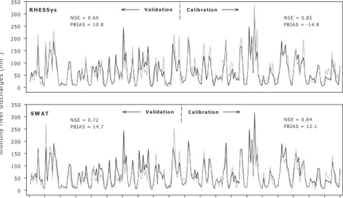
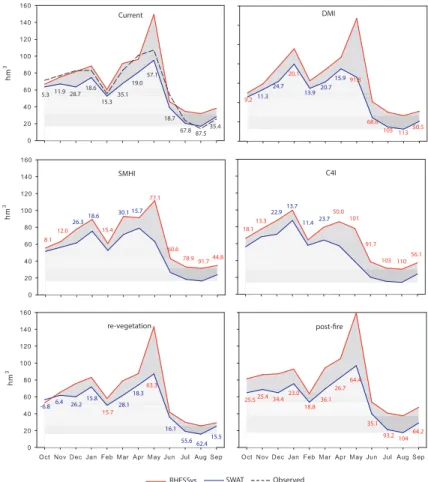
After calibration, performance of calibrated parameters needs to be assessed for an independent set of data (different time period) with no further adjustment of pa-rameters. This is referred to as “validation”, and for this work we selected the time
5
period 1986–1995. In Fig. 2 we show the performance of the two models after param-eter optimization, for the calibration and the validation periods. For both RHESSys and SWAT, simulated river flows show a high level of agreement with observations after the calibration of parameters, with NSE>0.8 for the calibration period and NSE≈0.7 for the validation period, and PBIAS values<15 % A little discordance between
mod-10
els is observed, however, according to PBIAS. While RHESSys slightly overestimates river flows for the calibration period and underestimate for the validation period, SWAT underestimates, on average, river flows for both calibration and validation periods. De-spite differences, both models are able to accurately simulate the water yield of the watershed, respecting the variability of river flows, and with small levels of bias.
15
3.4 Climate and land-use scenarios
The models were run and calibrated for observed climate, land-cover and soil types in the watersheds. For assessing the sensitivity of each model’s outputs to land-cover and climate changes, the models were then re-run (keeping constant the calibrated parameters) for a number of land-use scenarios and the outputs from various climate
20
models.
For climate change simulations we considered the outputs of three regional climate models (RCMs) for the time slice 2021–2050, from the ENSEMBLES project database (http://www.ensembles-eu.org/, Hewitt, 2004). This comprises a number of transient simulations of climate from 1950 to 2100 at high spatial resolution (25 km2 grid size;
25
time-HESSD
10, 11983–12026, 2013Senstitivity of water balance components
E. Morán-Tejeda et al.
Title Page
Abstract Introduction
Conclusions References
Tables Figures
◭ ◮
◭ ◮
Back Close
Full Screen / Esc
Printer-friendly Version Interactive Discussion
Discussion
P
a
per
|
D
iscussion
P
a
per
|
Discussion
P
a
per
|
Discuss
ion
P
a
per
slice with respect to control period (1970–2007). We selected the following RCM’s (driving Global Climate Model): C4I (HadCM3Q16), which projects the highest temper-ature increase (3.1◦C); DMI (ECHAM5-r3), which projects the lowest increase (1.1◦C); and SMHI (HadCM3Q3), which provides results located around the median (1.46◦C) of the temperature increase inter-model range. The three models show fairly good
sta-5
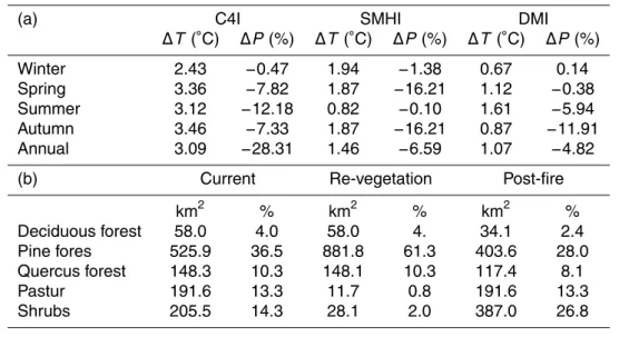
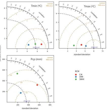
tistical agreement with observations for the control period for maximum and minimum temperatures. For precipitation only DMI is capable of reproducing the statistical char-acteristics of the observations, whereas C4I and SMHI present poorest performance (see the Taylor diagram in Fig. 3). Table 1a shows the projected changes in temperature and precipitation for each RCM.
10
The current land-use distribution in the watershed is the result of various anthro-pogenic and natural processes that have occurred during the last five decades, includ-ing the diminishinclud-ing and abandonment of rural activities such as croppinclud-ing and grazinclud-ing, or the afforestation of slopes for economic and environmental purposes. This has led to an expansion of forested area, which nowadays occupies nearly 50 % of the
wa-15
tershed’s area. The two other predominant land-uses are agricultural lands (14 %) in the valley bottom and sub-alpine pastures (13 %) in the high elevated areas of the watershed. Besides the current land-use scenario, two other potential scenarios were generated, based on realistic assumptions. On the one hand, we considered a fur-ther increase of altitudinal forest expansion. The current tree line is below its natural
20
limit due to human intervention in the past to gain land for feeding livestock. How-ever, currently land is undergoing afforestation as a consequence of reduced grazing and warmer temperatures (García-Ruiz et al., 2011). Therefore, the “re-vegetation sce-nario” includes the substitution of mountainous shrub and sub-alpine pasture by pine forests up to 2000 m, and the substitution of pastures by shrub (pine forest near the
25
tree line limit, therefore with shrub-like morphology) up to 2200 m (the altitude limit for
thePinus uncinata in the Pyrenees stands around 2200–2400 m according to
HESSD
10, 11983–12026, 2013Senstitivity of water balance components
E. Morán-Tejeda et al.
Title Page
Abstract Introduction
Conclusions References
Tables Figures
◭ ◮
◭ ◮
Back Close
Full Screen / Esc
Printer-friendly Version Interactive Discussion
Discussion
P
a
per
|
D
iscussion
P
a
per
|
Discussion
P
a
per
|
Discuss
ion
P
a
per
|
Mediterranean. Here we consider a post-fire scenario in a high altitude sector of the basin, in which forest has disappeared and shrub lands have colonized the soil, thus becoming the predominant feature of land-cover together with the mountainous pas-tures. The extension of each changing class for the different scenarios is shown in Table 1b.
5
The combination of the three land-use scenarios and the four climate scenarios (cur-rent and three RCMs), leads to 12 (1 baseline + 11 potential) scenarios, for which a number of water balance components were simulated, and compared between the two hydrological models The comparison of the different components was undertaken at two spatial scales: (1) the water yield (river discharges in hm3) comparison was
car-10
ried out for the entire watershed; (2) the surface runoff, snowpack water content, and evapotranspiration, were compared at a sub-basin scale, as this is the spatial unit at which the models generate those variables. We selected a sub-basin with relatively small size within the basin, to facilitate the performance of model runs and avoid the influence of stream flow aggregation processes which could mask the sensitivity of
15
water balance components to changing input conditions. The selected sub-basin in-cluded a mosaic of land-uses (deciduous forest, pine forest, shrub lands, pasture. . . ) and a high mean altitude. We focused on a high altitude sub-basin where snowfall and snowmelt occur to highlight the sensitivity of these processes to climate scenarios. The selected sub-basin is located in the north-west sector of the watershed (Fig. 1),
20
has 44.6 km2of extension and a mean altitude of 1580 m a.s.l.
4 Results
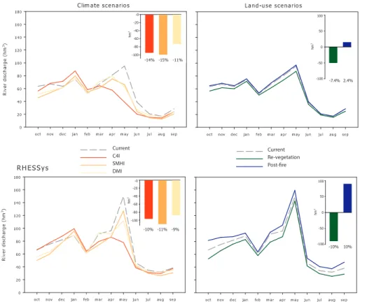
4.1 Changes in water yield at the watershed scale
Figure 4 shows the monthly and annual changes in water yield at the basin scale between the simulation for current conditions and the simulations for the climate and
25
HESSD
10, 11983–12026, 2013Senstitivity of water balance components
E. Morán-Tejeda et al.
Title Page
Abstract Introduction
Conclusions References
Tables Figures
◭ ◮
◭ ◮
Back Close
Full Screen / Esc
Printer-friendly Version Interactive Discussion
Discussion
P
a
per
|
D
iscussion
P
a
per
|
Discussion
P
a
per
|
Discuss
ion
P
a
per
first observe that the largest overall change is exhibited by the climate conditions sim-ulated by the SMHI model, with a decrease in annual water yield of 15 % and 13 % for the SWAT and RHESSys models respectively. The reason for this is that, as shown in Table 1b SMHI projects the largest decrease (16 %) of precipitation in autumn, which together with winter is the moist season of the year in the study area. Besides the
5
decrease in annual water yield, which is a common feature for all climate scenarios, the most manifest change is the loss of the spring peak flows, and the consequent in-crease of winter flows. This change is most remarkable for C4I, which is the model that projects the strongest warming at both seasonal and annual scales (Table 1b). Thus warmer temperatures will reduce the ratio of winter precipitation falling as snow and
10
will trigger an earlier melting of snowpack as well, thus explaining the observed shift in the hydrograph. To better appreciate the shift in the timing of flows under warmer con-ditions we have calculated the day of center of mass (Dcm: the day of the water year in
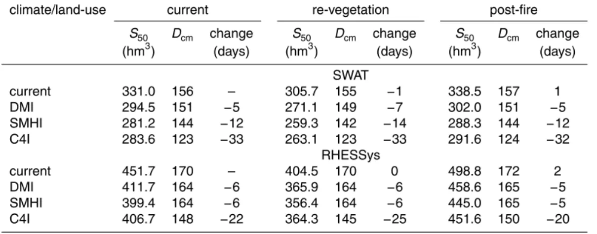
which the 50 % of the total streamflow occurs) for each scenario (Table 2). We thus ob-serve that for SWAT, in the most optimistic warming scenario scenario (DMI), the 50 %
15
of volume of water would be reached only 5 days earlier than under current conditions, whereas for the most pessimistic scenario (C4I), this would happen 33 days earlier, indicating a dramatic shift in the stream flows timing. For RHESSys the changes are less accentuated withDcm occurring 6 and 22 days earlier for DMI and C4I scenarios,
respectively. Although both SWAT and RHESSys show the same patterns of change
20
in water yield with varying climate conditions, this first results show that SWAT always projects a larger decrease in annual river flows than RHESSys, when forcing climate variables to change.
For the re-vegetation scenario (increase of forest altitude limit up to 2200 m) esti-mates show annual water losses of 7.4 % for SWAT and 10 % for RHESSys, with the
25
HESSD
10, 11983–12026, 2013Senstitivity of water balance components
E. Morán-Tejeda et al.
Title Page
Abstract Introduction
Conclusions References
Tables Figures
◭ ◮
◭ ◮
Back Close
Full Screen / Esc
Printer-friendly Version Interactive Discussion
Discussion
P
a
per
|
D
iscussion
P
a
per
|
Discussion
P
a
per
|
Discuss
ion
P
a
per
|
changes have to do with the impact of land-use on evapotranspiration, and in this case RHESSys produces larger changes than SWAT.
We thus see in a first approach that SWAT seems more sensitive to changes in cli-mate than RHESSys, and RHESSys is more sensitive to land-use change than SWAT in terms of the changes projected in water yield. In order to quantify these differences
5
we plot in Fig. 5 the seasonal (monthly-averaged) changes in stream flow for the 11 al-tered scenarios in comparison with the control scenario, for both SWAT (left-side semi-circles) and RHESSys (right-side semisemi-circles). An overall look at the plot confirms the previous observation (i.e. greater sensitivity of SWAT and RHESSys to climate change and land-use change, respectively). These model differences can also be seen when
10
combined climate and land-use scenarios are considered, and any decrease/increase in water yield will depend on the scenario and hydrological model considered. For example, in winter, SWAT shows larger water yield increase when only climate vari-ables are changed, but when considering a post-fire scenario the increase is larger for RHESSys for current and DMI climate scenarios. For the re-vegetation scenario,
15
increased forest cover counters the effects of increasing temperatures for both mod-els and a decrease of water yield is observed, except for the most extreme warming scenario (C4I). For the other seasons a decrease in water yield is evident for both RHESSys and SWAT and for all scenarios, except for the post-fire scenario. Thus for winter through summer, the models agree on the direction of change but differ only in
20
terms of the magnitude of change. For the post-fire scenario, model estimates differ both in the direction of change and in the magnitude of that change. In the case of SWAT, only when climate conditions remain unchanged, does the post-fire scenario show an increase in water yield; for RHESSys post-fire increases occur only for spring stream flows.
25
HESSD
10, 11983–12026, 2013Senstitivity of water balance components
E. Morán-Tejeda et al.
Title Page
Abstract Introduction
Conclusions References
Tables Figures
◭ ◮
◭ ◮
Back Close
Full Screen / Esc
Printer-friendly Version Interactive Discussion
Discussion
P
a
per
|
D
iscussion
P
a
per
|
Discussion
P
a
per
|
Discuss
ion
P
a
per
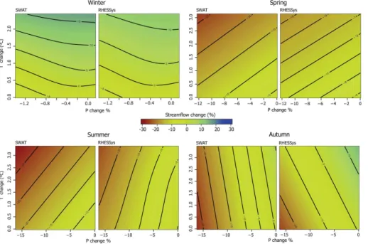
changing the climatic variables within the same range given by the RCMs, but only one or the other, i.e. changing seasonal temperatures according to values in Table 1a and maintaining current precipitation values, and vice versa. For an easier visual inter-pretation results of changes in stream flow were interpolated (using splines) in the 2-dimensional space, in order to create the surface plots of Fig. 6 in addition to the
5
greater amount of change in SWAT compared to RHESSys already mentioned, we also observe how the patterns of change differ among seasons and models, when considering changes in the climatic variables. In winter we observe how the precipita-tion change driven by RCMs is almost negligible, thus implying that the positive change in stream flow is driven essentially by the increase in temperatures. However the
sur-10
face trend shows how river flows start to increase only when temperature is raised by more than 0.5–1.0◦C. Below these values, precipitation is responsible for the decrease in stream flows. In the case of winter we observe how SWAT and RHESSys exhibit the same patterns of change, albeit with differences in magnitude. In spring, the same can be said for the SWAT and RHESSys intercomparisons (i.e. same pattern, different
15
magnitude) and we see how the pattern of change in stream flow is driven in an al-most symmetrical fashion by increasing temperatures and decreasing precipitation. In summer, we find the same pattern of change as in spring, i.e., a decrease in stream flow resulting from less precipitation and warmer temperatures (and thus enhanced evapotranspiration). However in the case of RHESSys the influence of temperatures
20
is smaller, as indicated for the more vertical contour lines of the plot. For autumn the pattern of change is opposite to that of spring. When decreasing precipitation, stream flows also decrease, whereas increasing temperatures have the opposite effect, i.e., increasing stream flows. The reason for this behavior is related to the effect of tem-peratures on snow accumulation. In late autumn (October–November) snowfalls are
25
HESSD
10, 11983–12026, 2013Senstitivity of water balance components
E. Morán-Tejeda et al.
Title Page
Abstract Introduction
Conclusions References
Tables Figures
◭ ◮
◭ ◮
Back Close
Full Screen / Esc
Printer-friendly Version Interactive Discussion
Discussion
P
a
per
|
D
iscussion
P
a
per
|
Discussion
P
a
per
|
Discuss
ion
P
a
per
|
precipitation will directly be converted to runoff, triggering the observed increase in au-tumn stream flows. This behavior is more evident for RHESSys than for SWAT, although again SWAT simulates the largest reduction of stream flow.
In this sub-section the different sensitivity of stream flow to land-use and climate changes between SWAT and RHESSys has been highlighted, and in general we have
5
demonstrated that SWAT produces larger changes in stream flow when climate vari-ables are forced to change while RHESSys yields greater changes when land-cover structure is changed. Taking into account that originally RHESSys produces an overall overestimation of flows and SWAT and overall underestimation (see PBIAS statistics in calibration) compared to observations, a systematic divergence between the two
mod-10
els is present. However, on the basis of results from these analyses, an increase or reduction of this divergence can be expected when considering the effects of climate and land-use changes on stream flow. Thus, in Fig. 7 we observe that under climate change scenarios, the divergence between SWAT and RHESSys usually decreases (blue figures) during the first half of the hydrological year, and drastically increases
15
(red figures) during the second half, especially in the peak flows of the spring and sum-mer. However, as temperature increases are higher (from DMI to C4I scenarios) there is a predominance of enhanced ranges of divergence between SWAT and RHESSys. In the re-vegetation scenario, the differences in results between the two models are gen-erally reduced when compared to the control simulations, and the opposite is observed
20
for the post-fire scenario.
4.2 Changes in water balance components at the sub-basin scale
The most remarkable changes observed under climate and land-use scenarios are the shifting of spring peak flows when increasing temperatures, the loss of water yield given by reduced precipitation, or the increase/decrease of water yield when land-cover
sce-25
HESSD
10, 11983–12026, 2013Senstitivity of water balance components
E. Morán-Tejeda et al.
Title Page
Abstract Introduction
Conclusions References
Tables Figures
◭ ◮
◭ ◮
Back Close
Full Screen / Esc
Printer-friendly Version Interactive Discussion
Discussion
P
a
per
|
D
iscussion
P
a
per
|
Discussion
P
a
per
|
Discuss
ion
P
a
per
plants surface plus the water transpired by plants), are essential water balance compo-nents for understanding the processes underlying the observed stream flow changes.
For a better assessment of the behavior of water balance components under chang-ing conditions a second set of analyses have been conducted at the sub-basin scale. In particular, this enables the effects of land-cover changes on stream flow to be analyzed
5
in depth, as the proposed changes have a greater magnitude (in relative terms) in the selected sub-basin than in the whole watershed. In addition, the contribution of snow-fall/snowmelt, surface runoffand evapotranspiration is better assessed at this smaller scale.
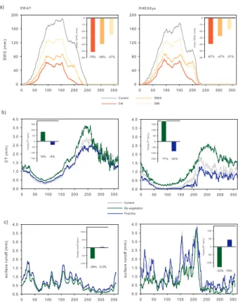
Figure 8a shows the daily (long-term average) snowpack water content (snow water
10
equivalent, SWE, in mm) in the sub-basin and the change in the mean yearly val-ues, between the control period and the three climate scenarios. We observe that for the control simulation, SWAT produces slightly greater values of SWE than RHESSys. However, when climate-change scenarios are considered, the amount of SWE de-creases drastically, and as already seen for the stream flow analyses, the decrease
15
is more pronounced for SWAT than for RHESSys. In this case, it is evident that the decrease in the amount of snow is closely related to the increase in temperatures in-duced by the climate models, as C4I (DMI) produces the greatest (smallest) loss of SWE. In Fig. 8b, the average amount of water loss by evapotranspiration (ET) from the subbasin simulated by SWAT and RHESSys is shown. Although the seasonal pattern
20
is similar for the two models, we observe that SWAT produces higher values of ET throughout the year, this being the possible cause for lower stream flows simulated by SWAT than by RHESSys. When considering the two land-use scenarios, the changes in ET are much more pronounced for RHESSys than for SWAT, the first (latter) showing a yearly increase of 71 % (19 %) for the re-vegetation scenario and a decrease of 34 %
25
(−6 %) for the post-fire scenario. These differences also seem to explain the greater
HESSD
10, 11983–12026, 2013Senstitivity of water balance components
E. Morán-Tejeda et al.
Title Page
Abstract Introduction
Conclusions References
Tables Figures
◭ ◮
◭ ◮
Back Close
Full Screen / Esc
Printer-friendly Version Interactive Discussion
Discussion
P
a
per
|
D
iscussion
P
a
per
|
Discussion
P
a
per
|
Discuss
ion
P
a
per
|
between models are even larger. The two models reproduce the same intra-annual vari-ability; however, RHESSys yields larger amounts of runoffthan SWAT. When changing land-use the two models respond in the same manner, i.e. decreasing runofffor the re-vegetation scenario, and increasing runoff for post-fire scenario, but again RHESSys produces the largest amount of change.
5
The effect of land-cover changes on stream flow are well captured by the models, although RHESSys shows more sensitivity than SWAT. A last experiment was carried out in order to investigate more thoroughly the response of water yield and evapotran-spiration to changes in land-cover, and to assess differences between the two models. In the selected sub-basin, the land-use “pasture” was substituted by “pine forest”
grad-10
ually i.e. 10 % of pasture extension into forest, 20 %, 30 % . . . and up 100 %. For each of these 10 land-use scenarios the water yield and the mean evapotranspiration of the basin were compared with current land-use scenario. Figure 9 shows the results in relative changes for the monthly (surface plots) and yearly (line plots). As expected, the changes generated by RHESSys are of greater magnitude than those of SWAT.
15
However, the major insight from this analysis is the evidence of a different behav-ior of the hydrological variables between the two models, when the forest expansion is increased in a linear way. The monthly pattern of change shows that the greatest decrease (in relative terms) in stream flow occurs in summer months for SWAT and between late summer and winter for RHESSys. Moreover, whereas SWAT yields a
de-20
crease in stream flow for all months and all scenarios, in RHESSys a slight increase is observed in spring months when pasture is change into forest up to a 50 % level. When looking at the yearly changes (right plots) we observe that the response of stream flow to increased forest cover is perfectly linear for SWAT. RHESSys on the contrary, shows a more complicated pattern with the slope of the curve (intensity of flow decrease)
be-25
HESSD
10, 11983–12026, 2013Senstitivity of water balance components
E. Morán-Tejeda et al.
Title Page
Abstract Introduction
Conclusions References
Tables Figures
◭ ◮
◭ ◮
Back Close
Full Screen / Esc
Printer-friendly Version Interactive Discussion
Discussion
P
a
per
|
D
iscussion
P
a
per
|
Discussion
P
a
per
|
Discuss
ion
P
a
per
in RHESSys again from the 50 % change of pasture to forest. On a monthly basis, the two models yield a similar pattern of change in ET, but the amount of increase for RHESSys is one order of magnitude greater than for SWAT (see the values of color scale).
5 Discussion
5
Substantial research has been carried out in the field of hydrology in order to predict the future behavior of river flows under changing environmental conditions, especially in the climate variables and the land-cover distribution. The process-based hydrolog-ical models are the most widely used tool for hydrologhydrolog-ical forecasting in both scien-tific and management fields, as they allow simulating through physical relationships
10
a number of processes and variables that integrate the water cycle. In general terms, a decrease of river flows can be expected according to the two models used in this work, if climate and land-use evolve as predicted. The process of re-vegetation in the studied area and other Mediterranean mountains is likely to continue in the manner discussed in this paper, i.e. shrubs evolving to forest and sub-alpine pastures being
15
colonized by shrubs (García-Ruiz and Lana-Renault, 2011; García-Ruiz et al., 2011). Moreover, climate projections agree in emphasizing the fact that the Mediterranean will become a hotspot of climate warming in future decades (Solomon et al., 2007; Giorgi, 2006) and mountains are expected to suffer both an increase in temperatures and a decrease in precipitation (Bravo et al., 2008). According to the SWAT model, climate
20
change will have greater impacts on the availability of water resources than land-cover changes. This fact has been emphasized by Koeplin et al. (2013) in a study on the Swiss Alps, although the latter will be affected by increasing glacier melting, which is not the case of the Pyrenees. Similar conclusions have been reported in other areas of the world when simulating stream flows under climate and land-cover scenarios with
25
HESSD
10, 11983–12026, 2013Senstitivity of water balance components
E. Morán-Tejeda et al.
Title Page
Abstract Introduction
Conclusions References
Tables Figures
◭ ◮
◭ ◮
Back Close
Full Screen / Esc
Printer-friendly Version Interactive Discussion
Discussion
P
a
per
|
D
iscussion
P
a
per
|
Discussion
P
a
per
|
Discuss
ion
P
a
per
|
on water resources than changes in the climate variables, in this specific environment. This highlights the importance of considering the combination of scenarios in order to understand the range of impacts of environmental changes in the future availability of water resources (Tong et al., 2012; Koeplin et al., 2013).
Despite the good performance of hydrological models to simulate stream flows in
5
a range of environments, a number of uncertainties nevertheless remain. One of the aims of this work has been to highlight the fact that another source of uncertainty in hydrological forecast resides in the choice of the hydrological model to be used. The two compared models have been previously applied in mountainous environments, and seem adequate to simulate water yield and other hydrological variables under changing
10
conditions at different spatial scales. RHESSys has been successfully applied to sim-ulate transpiration (Christensen et al., 2008), to assess the impacts of climate change on water yield (Zierl and Bugmann, 2005) or to simulate snow distribution in diff er-ent mountain regions of the world (Hartman et al., 1999), amongst other applications. SWAT, which was primarily developed for improving agricultural and irrigation
manage-15
ment, has been successively updated and is able to reproduce the water cycle in moun-tainous and snow-dominated environments (Fontaine et al., 2002; Rahman et al., 2013; Pradhanang et al., 2011; Debele et al., 2010; Zhang et al., 2008). We demonstrate that even when the two models have been calibrated, and therefore can satisfactorily re-produce the stream flows of a given river basin, their forecast for future availability of
20
water under hypothetical climate and land-use conditions may differ substantially from each other. Although the direction of changes estimated by the models was usually consistent, the magnitudes of these changes were substantially different. In the case of this study, SWAT tends to produce larger changes in hydrological variables under induced changes in climate variables, and RHESSys tends to produce larger
hydro-25
HESSD
10, 11983–12026, 2013Senstitivity of water balance components
E. Morán-Tejeda et al.
Title Page
Abstract Introduction
Conclusions References
Tables Figures
◭ ◮
◭ ◮
Back Close
Full Screen / Esc
Printer-friendly Version Interactive Discussion
Discussion
P
a
per
|
D
iscussion
P
a
per
|
Discussion
P
a
per
|
Discuss
ion
P
a
per
sensitivity to climate and especially to land-use change. To provide examples we ana-lyzed, at the sub-basin scale, the behavior of different variables (snow water equivalent, evapotranspiration and surface runoff) that are essential components of the water bal-ance. Regarding ET, we observe that it is the key element for understanding the effect of land-use changes on water yield. Forest expansion enhances evapotranspiration
5
given the larger surface of plant canopy to retain water from precipitation (interception) as well as for the increased amount of water used by plants for their biological activity (Crockford and Richardson, 2000; Zhang et al., 2001). This consequently implies less water available for runoffand an overall decrease in the catchment water yield. Our re-sults indicate that ET and water yield show a linear response when forest is gradually
10
increased in the SWAT model, and a non-linear response is observed for RHESSys, where an abrupt change is observed once a certain threshold of forest increase is reached. These differences in ET estimates are most likely related to the way that both models compute actual evapotranspiration. SWAT estimates actual evapotranspi-ration through empirical equations and as a function of potential evapotranspievapotranspi-ration,
15
water held in plant canopy or sublimation amongst other variables. On the contrary RHESSys has a more process-based evapotranspiration estimate, with a more com-plex representation of canopy controls on transpiration, through stomatal conductance, a time-varying rooting depth and sunlit and shaded leaves. While this representation may be more physiologically realistic it also requires additional parameterization that
20
can introduce further error. Testing of model estimates against measured evapotranspi-ration data across a range of vegetation types would be required to determine whether or not the additional physiological realism in RHESSys actually produces more accu-rate estimates, relative to SWAT. Regarding snow, both models simulate a decrease of SWE when climate scenarios are considered, and this seems to be the main cause for
25
HESSD
10, 11983–12026, 2013Senstitivity of water balance components
E. Morán-Tejeda et al.
Title Page
Abstract Introduction
Conclusions References
Tables Figures
◭ ◮
◭ ◮
Back Close
Full Screen / Esc
Printer-friendly Version Interactive Discussion
Discussion
P
a
per
|
D
iscussion
P
a
per
|
Discussion
P
a
per
|
Discuss
ion
P
a
per
|
is already a fact in many snow-dominated areas of the Mediterranean (García-Ruiz et al., 2011), and further changes in the future may require substantial modifications in the management of the numerous reservoirs in the region (López-Moreno et al., 2008), as the one located downstream of the studied area. Our estimates show greater reduc-tion in snow with climate scenarios found using SWAT. Again, the RHESSys model is
5
more physically realistic – accounting for both radiation and temperature driven melt –, but again further analysis would be needed to determine whether the additional param-eterization associated with this complexity actually produces more accurate results.
It must be taken into account as well the original conception of the models, as RHESSys was conceived for simulating carbon, water and nutrients cycling in natural
10
environments, whereas SWAT was in principle oriented to model water, sediment, or contaminant yields in crops and managed watersheds (Tague and Band, 2004; Neitsch et al., 2005). The question that arises from this observation is to what extent these di-vergences can be considered an overestimation or an underestimation from one model to another. In other words, is SWAT overestimating hydrological changes under climate
15
conditions, or is RHESSys underestimating them? (The same argument is applicable to land-use changes). The answer to this question is difficult to provide based on the observations of this study, thus it certainly requires further research, and even com-parisons with additional hydrological models in other areas and environments In the meanwhile it is the responsibility of model users to assess the uncertainty associated
20
to model predictions and recognize the strengths and limitations of the model used. Finally, our observations highlight that the degree of divergence (which can be con-sidered as a degree of uncertainty) in the forecasted stream flow between the two models may be enhanced or reduced depending on the combination of climate change and land-use change scenarios This can also be related to the calibration process. In
25
HESSD
10, 11983–12026, 2013Senstitivity of water balance components
E. Morán-Tejeda et al.
Title Page
Abstract Introduction
Conclusions References
Tables Figures
◭ ◮
◭ ◮
Back Close
Full Screen / Esc
Printer-friendly Version Interactive Discussion
Discussion
P
a
per
|
D
iscussion
P
a
per
|
Discussion
P
a
per
|
Discuss
ion
P
a
per
extent in RHESSys, therefore the uncertainty range (i.e., the divergence between the two models) is in this case reduced. The opposite is observed when vegetation is re-moved. For the case of climate change scenarios the pattern is less clear but there is a trend towards increasing uncertainty when the projections for temperature increase are more severe (i.e., the C4I scenario). This circumstance could be different for
ex-5
ample if other sets of parameterization had been used, in which the bias of modeled stream flow with respect to observations were of different magnitude or sign. This leads to the concept of “equifinality” (Beven, 2006) which in hydrological modeling refers to the possibility that different solutions or sets of model parameterizations may lead to op-timal model performance, and it is considered as an important component of a model’s
10
uncertainty. It was not our intention in this work to evaluate the performance of dif-ferent calibration solutions, but this will be done in further research in order to better understand the uncertainties related to hydrological modeling.
6 Conclusions
The components of water balance, including stream flow, evapotranspiration and
snow-15
pack water content were simulated for a Pyrenean watershed to assess its sensitivity to changes in climate and land-use change. Under climate change conditions (increas-ing temperatures and decreas(increas-ing precipitation), stream flows will suffer reductions and shifting peak flows, leading to a dramatic change in the shape and magnitude of the hydrographs, which depends on the degree of severity of the climate scenario
consid-20
ered. When two hypothetical (but plausible) land-use scenarios are considered, stream flows (and evapotranspiration) are affected as well, i.e. a decrease of river flows and an increase in evapotranspiration are observed in the case of a re-vegetation scenario, and the opposite effect is observed when a post-fire vegetation scenario is considered. The principal highlight of this work is the demonstration that model choice in
gen-25