www.geosci-model-dev.net/3/309/2010/
© Author(s) 2010. This work is distributed under the Creative Commons Attribution 3.0 License.
Geoscientific
Model Development
Assessment of bias-adjusted PM
2
.
5
air quality forecasts
over the continental United States during 2007
D. Kang1, R. Mathur2, and S. Trivikrama Rao2
1Computer Science Corporation, Research Triangle Park, 79 T.W. Alexander Drive, NC 27709, USA 2Atmospheric Modeling and Analysis Division, National Exposure Research Laboratory,
US Environmental Protection Agency, Research Triangle Park, NC, USA
Received: 29 October 2009 – Published in Geosci. Model Dev. Discuss.: 8 December 2009 Revised: 7 April 2010 – Accepted: 8 April 2010 – Published: 16 April 2010
Abstract. To develop fine particulate matter (PM2.5) air quality forecasts for the US, a National Air Quality Forecast Capability (NAQFC) system, which linked NOAA’s North American Mesoscale (NAM) meteorological model with EPA’s Community Multiscale Air Quality (CMAQ) model, was deployed in the developmental mode over the conti-nental United States during 2007. This study investigates the operational use of a bias-adjustment technique called the Kalman Filter Predictor approach for improving the accuracy of the PM2.5forecasts at monitoring locations. The Kalman Filter Predictor bias-adjustment technique is a recursive algo-rithm designed to optimally estimate bias-adjustment terms using the information extracted from previous measurements and forecasts.
The bias-adjustment technique is found to improve PM2.5 forecasts (i.e. reduced errors and increased correlation coeffi-cients) for the entire year at almost all locations. The NAQFC tends to overestimate PM2.5during the cool season and un-derestimate during the warm season in the eastern part of the continental US domain, but the opposite is true for the Pacific Coast. In the Rocky Mountain region, the NAQFC system overestimates PM2.5 for the whole year. The bias-adjusted forecasts can quickly (after 2–3 days’ lag) adjust to reflect the transition from one regime to the other. The modest computational requirements and systematic improve-ments in forecast outputs across all seasons suggest that this technique can be easily adapted to perform bias adjustment for real-time PM2.5air quality forecasts.
Correspondence to:D. Kang ([email protected])
1 Introduction
and unique data set for performing comprehensive evalua-tions of bias-corrected pollutant fields.
While it is recognized that PM2.5 pollution results from both primary emissions and secondary formation through complex photochemical and heterogeneous chemical path-ways, significant scientific and technical challenges sur-round the characterization of ambient PM2.5 distributions both through modeling and measurements (e.g., McMurry, 2000; Donahue et al., 2009). The emissions and physical, chemical, and removal processes controlling day-to-day lev-els of ambient PM2.5and precursor concentrations also ex-hibit seasonal variability, resulting in significant spatial and seasonal variability in ambient PM2.5mass and its chemical composition. Current uncertainties in these individual com-ponents pose enormous challenges for developing accurate short-term PM2.5 forecasts (Mathur et al., 2008; Yu et al., 2008). Nevertheless, a need exists for local air quality agen-cies to provide accurate forecast of PM2.5concentrations to alert the sensitive population on the onset and duration of unhealthy air associated with elevated PM2.5levels. To ad-dress this need, the utility of PM2.5 forecast guidance ob-tained from comprehensive atmospheric models can, in the short-term, be improved through post-processing of forecast output with bias-adjustment methods; this is the primary mo-tivation for the analysis presented in this study. It should be noted that post-processing bias-adjustment techniques are routinely used in conjunction with numerical weather pre-diction models, despite decades of research to improve the formulations in the meteorological models, to develop more accurate forecast products (Glahn and Lowry, 1972; http: //www.weather.gov/mdl/synop/products.php). Given the rel-atively early state of PM2.5forecast models and large uncer-tainties in process representations, the exploration of bias-adjustment techniques to improve the usefulness of PM2.5 forecasts is warranted.
Different adjustment (also referred to as bias-correction) techniques have been used for improving surface O3predictions in recent years (McKeen et al., 2005; Delle Monache et al., 2006; Wilczak et al., 2006; Delle Monache et al., 2008; and Kang et al., 2008). Among these techniques, the Kalman Filter (KF) predictor (hereafter referred to as KF bias-adjustment or simply KF) forecast method yielded the most forecast skill improvement. Kang et al. (2008) pre-sented the application of KF technique to O3forecasts over the continental US domain for a three-month period from July to September 2005. While the technique was found to improve the forecast skill for O3, it was not clear if they would be readily applicable for PM forecasts and whether they would yield similar improvements in PM forecast skill. This is primarily due to the fact that unlike O3, elevated PM2.5 concentrations are encountered throughout the year and that significant seasonal biases exist in current mod-els both in the representation of total PM2.5 mass as well as its composition (cf. Mathur et al., 2008; McKeen et al., 2007; Appel et al., 2008). Additionally, the chemical
con-stituent contributing to the bias could also vary both spatially and seasonally. Thus, for improved PM forecasts, the bias-adjustment techniques should be capable of correcting biases and errors that not only change with time, but that also may have widely varying sources of origin.
In this study, the KF bias-adjustment technique is applied to PM2.5forecasts for the year of 2007 over the continental US domain. To our knowledge, this is the first comprehen-sive assessment of the bias-adjustment technique for PM2.5 forecasts. Within the continental US domain, there are about 500 AIRNow sites that report hourly PM2.5 concentrations which are measured using the Tapered Element Oscillating Microbalance (TEOM) method. The year-long forecast pe-riod over the continental US has provided a unique data set covering a wide range of atmospheric conditions and a broad PM2.5 concentration range to test the performance of the bias-adjustment technique for PM2.5forecasts.
The objectives of this study include: (1) apply the KF post-processing technique to improve skills for real-time PM2.5 forecasts, (2) investigate the spatial and temporal character-istics of this technique when applied to PM2.5forecasts, and (3) analyze the impact of bias adjustment on forecast errors of different types (e.g., systematic versus unsystematic). Sec-tion 2 describes the modeling system, the implementaSec-tion of the KF bias-adjustment technique, observational data, and evaluation metrics. In Sect. 3 the performance evaluation results and discussions are presented. And the results and conclusions are summarized in Sect. 4.
2 Experiments and methods
2.1 The NAQFC system
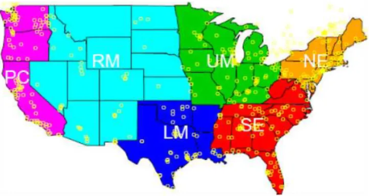
Fig. 1. Analysis sub-regions and monitoring sites (AIRnow net-work), the horizontal domain is discretized with a 442×265 12 km
grid cells. NE: Northeast, SE: southeast, UM: Upper Midwest, LM: Lower Midwest, RM: Rocky Mountains, PC: Pacific Coast.
on the Lambert Conformal map projection and 22 vertical layers of variable thickness set on a sigma coordinate rang-ing from the surface to 100 hPa. Since the PM2.5forecasts were in the developmental stage, changes or modifications to the AQF components were allowable to accommodate new developments reflecting evolving science. For instance, on 17 September 2007, the treatment for the PBL mixing height scheme in CMAQ was changed from the Turbulence Ki-netic Energy (TKE)-based method to the Asymmetric Con-vective Model-2 (ACM2)-based method, which on average decreased the PBL depth, helping reduce forecast errors for both O3and PM2.5in the Pacific Coast region. However, this study does not deal with the impacts of the various changes or modifications to the forecast model; rather, it focused on how the bias-adjustment technique can improve the forecast re-sults over the raw model forecasts. Since the bias-adjustment technique employed in this study is statistical type, it does not involve any modifications in the physical and chemical processes treated in the forecast model.
The emissions inventories used by the AQF system were updated from the US EPA’s 2001 national emission inventory to represent the 2007 forecast year (Eder et al., 2009). The biogenic emissions were processed using Biogenic Emis-sion Inventory System (BEIS) verEmis-sion 3.13 (Schwede et al., 2005). Emissions from sea salt, wild fires, and wind-blown dust were not considered for the AQF system, which may contribute to the underestimation of PM2.5 forecasts under some circumstances. The Carbon Bond chemical mechanism (version 4.2) is used to represent the photochemical reactions and AERO3 aerosol module is used to represent aerosol for-mation and distribution. The chemical fields for CMAQ are initialized using the previous forecast cycle. The primary NAM-CMAQ model forecast for the next 48-h surface-layer PM2.5 is based on the current day’s 06:00 UTC cycle, and this is the only cycle available for the developmental PM2.5 forecasts.
2.2 Observations
Hourly, near real-time, PM2.5 measurements (µg/m3) ob-tained from EPA’s AIRNow program are used in this study (http://www.epa.gov/airnow). All measurements are made using TEOM instruments and concentrations are averaged over hourly intervals from the beginning of one hour to the next. It should be recognized that TEOM measurements are somewhat uncertain and are believed to be lower limits to a “true” value because of volatilization of semivolatile ma-terial (ammonium nitrate and organic carbon) in the drying stages of the measurement (Eatough et al., 2003; Grover et al., 2005). Nevertheless, the TEOM measurements are the only real-time hourly PM2.5 observation data available for use in the purpose of this study. About 500 PM2.5 monitor-ing stations are available within the continental US domain (Fig. 1) for the year of 2007. For verification purposes and forecast products, the daily (24-h) mean PM2.5 concentra-tions are often used.
2.3 Implementation of the KF bias-adjustment method
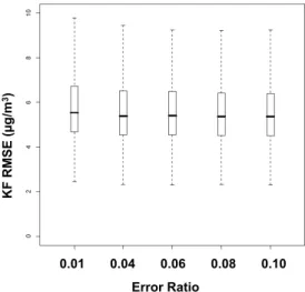
The KF predictor bias-adjustment algorithm (Kalman, 1960) was described in detail by Delle Monache et al. (2006) and a concise description of its implementation was provided by Kang et al. (2008). The specification of the error ratio, a key parameter in the KF approach which determines the relative weighting of observed and forecast values, was previously investigated extensively for O3forecasts. Even though the optimal error ratios were found to vary across space, the im-pact of using different optimal values over the model domain on the resultant bias-adjusted O3 predictions was insignif-icant when compared to using a representative fixed value across all locations (Kang et al., 2008). To test whether the same conclusion is valid for the PM2.5forecasts, error ratios ranging from 0.01 to 0.10 were selected to perform PM2.5 forecasts for all the sites across the domain over the entire year, and RMSE values were calculated at each site to gauge the impact of spatially different error ratio values on the fore-cast performance. As shown in Fig. 2, the impact of different error ratio values ranging from 0.04 to 0.10 on the forecast performance is small, and only when the error ratio of 0.01 was used, the RMSE values were relatively larger than using other values. Hence, in this study, we used the same single fixed error ratio value of 0.06 at all the locations for devel-oping bias-adjusted PM2.5forecasts. In these plots (and also applies to all the boxplots in this paper), the metric is calcu-lated at each site for the specific period and then is presented across all the sites within a region or the entire domain as a box plot, with the lower and upper borders of the box rep-resenting the first and third quartiles while the middle line represents the median value.
0.01 0.04 0.06 0.08 0.10
Error Ratio
KF RMSE (µg/m
3)
Fig. 2. Impact of error ratios on the performance (RMSE) of
Kalman Filter adjusted forecasts for the daily mean PM2.5
concen-trations (µg/m3).
hourly observations and raw model predictions for the prior 2 days. Then the updated parameters and the third day’s raw model forecasts are used to create bias-adjusted forecasts for the 3rd day. All updated KF parameters for each hour and at each site are saved into a file for use in the subsequent KF run. The KF runs then continue by reading the previ-ous day’s KF parameters and observations and raw model predictions from the prior 2 days to generate the next day’s bias-adjusted forecasts by combining with the next day’s raw model forecasts. Thus, in developing the daily KF forecasts, if data for two consecutive days are missing at a site, the KF will automatically drop this site from future bias-adjustment forecasts; however, if a new site with two consecutive days’ data appears in the observation data set, the KF will initial-ize the site with initial values of KF parameters and generate bias-adjusted forecasts further onward. This implementation is adaptable in real-time to the variable nature of monitoring stations which report hourly observations to the AIRNOW network and can be easily combined with AQF system to produce real-time bias-adjusted forecasts.
2.4 Verification statistics and spatial-temporal considerations
To assess the performance of the KF bias-adjusted forecasts, a variety of statistical metrics are used, including Root Mean Square Error (RMSE) and its systematic and unsystematic components, Normalized Mean Error (NME), Mean Bias (MB), Normalized Mean Bias (NMB), correlation coefficient (r), and Index Of Agreement (IOA). For a forecast product, it is also important to evaluate its performance over categorical forecasts (Kang et al., 2005). Two categorical metrics, False Alarm Ratio (FAR) and Hit Rate (H), are used in this study.
Mean Daily PM
2.5
(µg/m
3)
50 100 150 200 250 300 350
Day of the Year (1/15/07-12/30/07)
5 10 15 20 25
Fig. 3. Time series of observed, raw model forecast, and KF
bias-adjusted forecast daily mean PM2.5(µg/m3). OBS: observations,
KF: Kalman filter bias-adjustment, MOD: raw model.
Since the NAQFC domain covers the continental United States and given large region-to-region differences in the physical and chemical processes, the continental US domain is divided into six subregions following US state boundaries to facilitate the performance evaluations (Fig. 1). The four easternmost subregions, northeast (NE), southeast (SE), up-per Midwest (UM), and lower Midwest (LM), are based on O3and other chemical species climatology that identified ar-eas of homogeneous variability using principal component analysis (Eder et al., 1993; Gego et al., 2005). The domain-wide statistics are calculated using all the observations avail-able within the domain.
Figure 3 presents comparisons of time series of the domain-wide daily average observed, raw model forecasts, and KF bias-adjustment forecasts of PM2.5 concentrations during 2007. As shown in Fig. 3, the raw model tends to overpredict during the cool season (before mid-April and af-ter August) and underpredict during the warm season (mid-April to end of August) when compared with observations. To facilitate the temporal performance evaluations, the time series are divided into cool season (from January to 20 April and from September to December) and warm season (from 21 April to 31 August).
3 Results
3.1 General performance
50 100 150 200 250 300 350
Day of the Year (1/15/07-12/30/07)
Mean
Dail
y
PM
2.5
(µg/
m
3)
5 10 15 20 25 30
5 10 15 20 25 30
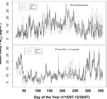
Fig. 4. Time series of observed, raw model forecast, and KF
bias-adjusted forecast daily mean PM2.5(µg/m3)at Southeast and
Pa-cific Coast.
a transitional period from underestimation to overestimation. From early September until the end of the year, the overesti-mation of the raw model became larger. This is partially at-tributed to the change of the PBL mixing scheme for CMAQ on 17 September, as mentioned before. Nevertheless, the KF bias-adjustment technique could quickly respond to the tran-sitions from one regime to another and tracked the observa-tions well in the time series. Since Fig. 3 presents the aggre-gate results for the entire domain, some important informa-tion may be hidden due to smoothing during the averaging process. Figure 4 displays same time series as Fig. 3 for two representative sub-regions: Southeast and Pacific Coast. The time series for the Southeast resembles that of the do-main, with raw model overestimating during cool season and underestimating during the warm season. However, the un-derestimation during the warm season is more pronounced for the Southeast than for the entire domain. The time se-ries of the Pacific Coast reveals a completely different story, in which the raw model generally over-predicted during the cool season and under-predicted during the warm season. The over-prediction was much stronger at the beginning of the year (January and early February) than that over the rest of cool season. The over-prediction for the later cool sea-son (from September to December) was reduced, and during most times the raw model could reproduce the observations quite well. The performance change of the raw model during cool season is attributable to the adoption of the new PBL mixing height parameterization when the TKE-based PBL height was replaced by the ACM2-based PBL height. The ACM2-based PBL height generally leads to higher PM2.5 concentrations than the TKE-based PBL height since the
(a) R2 = 0.43 (b) R2 = 0.90
Observed Daily Mean PM2.5 (µg/m3)
Model Daily Mean PM
2.5
(µg/m
3)
Model Daily Mean PM
2.5
(µg/m
3)
Fig. 5.Scatterplots between forecasts and observations for selected
percentiles for the daily mean PM2.5concentrations (µg/m3): (a)
raw model forecasts,(b)Kalman filter-adjusted forecasts.
ACM2-based PBL height is generally lower than the TKE-based PBL height. The under-prediction is thus reduced for the west region of the domain during the cool season, but the over-prediction is further aggravated for the eastern part of the domain during the same period. Nonetheless, the time se-ries of the KF bias-adjusted predictions tracked the observed time series better than the raw model predictions.
To further investigate the performance of the KF bias-adjusted forecasts and compare with the raw model forecasts, Fig. 5 displays the scatter plots of forecast and observed val-ues across various percentiles for the daily mean PM2.5for all the stations within the continental US domain. Follow-ing Mathur et al. (2008), at each site the time series of both measured and model (or KF bias-adjusted model) daily mean PM2.5over the entire year was examined and percentiles of the distribution over the study period were computed for both modeled and observed values. Scatter plots of specific per-centiles of the concentration distributions (e.g., median) of the model and observed time series are then examined to as-sess the ability of the model to capture the spatial variability in frequency distributions of PM2.5concentrations across the sites (Mathur et al., 2008). As shown in Fig. 5, compared with the raw model forecasts (left), the KF bias-adjusted forecasts displayed a much better match with the observed distributions as reflected by the reduced scatter about the 1:1 line, especially for the higher percentiles. The overall corre-lation between model forecasts and observations was greatly improved with the value ofR2increasing from 0.43 for the raw model forecasts to 0.90 for the KF bias-adjusted fore-casts. Similar improvements in O3forecasts after the appli-cation of the KF bias adjustment were previously reported in Kang et al. (2008).
Density
Daily mean PM2.5(µg/m3)
(a)
(b)
(c)
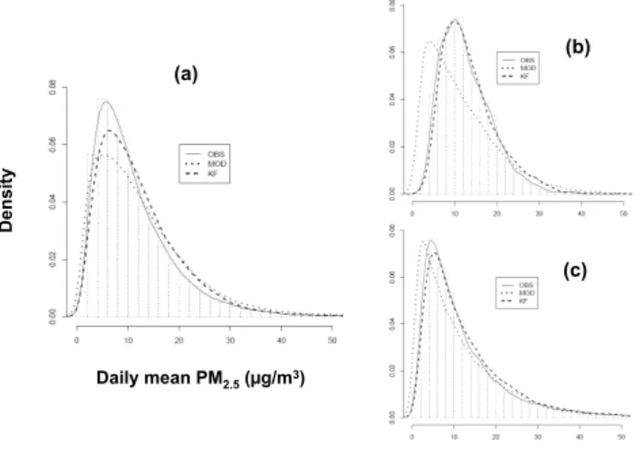
Fig. 6.The histogram of observed and the fitted Gaussian
probabil-ity densprobabil-ity function of observed, raw model forecast, and KF fore-cast daily mean PM2.5concentrations (µg/m3): (a)Domain over
entire year,(b) LM during warm season, and(c)PC during cool season.
distribution for the entire domain during 2007, while Fig. 6b presents the distribution for Lower Midwest during the warm season and Fig. 6c for Pacific Coast during the cool season to typify the sub-regional and seasonal signals. As seen in Fig. 6, the KF technique brings the PDFs of forecast values much closer to those of the observations. The improvements are more pronounced in the sub-regional and seasonal bution comparisons illustrated in Fig. 6b and c. The distri-butions of the raw model forecasts for both cases were out of phase compared to those of the observations, especially for Lower Midwest during the warm season. The KF bias-adjusted forecasts were able to reproduce the observations very well in both cases.
3.2 Regional performance
Tables 1 and 2 present the domain and sub-regional sum-mary of discrete statistics for the raw model and the KF bias-adjusted daily mean PM2.5forecasts during the cool and warm seasons, respectively. Examination of Table 1 reveals that during the cool season, the RMSE values range from 7.2 to 11.4 (µg/m3)for the raw model forecasts, and from 5.2 to 7.6 (µg/m3)for the KF bias-adjusted forecasts; this translates to about a 20% reduction in RMSE as a result of the application of the bias adjustment. Similar reductions are also noted for the NME. The MB and NMB indicate that during the cool season, the raw model systematically over-predicted daily mean PM2.5across all the sub-regions except the Pacific Coast where it under-predicted. The KF bias-adjusted forecast reduced NMB values across all the sub-regions. Correlation coefficients also increased significantly across all the regions as a result of the bias adjustment, with the largest increase in the LM and RM regions. The summary statistics during the warm season (Table 2) indicate
compara-ble improvement in the error statistics (RMSE and NME) for the KF bias-adjusted forecasts relative to the raw model. In contrast to the cool season, systematic under-predictions are noted in the warm season raw model PM2.5forecasts (Mathur et al., 2008). The application of the KF bias adjustment helps reduce both the cool season high bias and the warm season low bias, and also results in consistently improved correla-tions with measurements across all seasons.
Figure 7 presents comparisons of the distribution of monthly RMSE values of daily mean PM2.5 for the raw model and KF forecasts for the different sub-regions. As seen in Fig. 7, the RMSE values are consistently lower for the KF forecasts relative to those of the raw model across all sub-regions and months. In addition, the error distribu-tion range (the size of the boxes) for the KF forecasts is also much smaller than the raw model forecasts. During October– December, the raw model forecasts exhibited large RMSE values for both the UM and LM sub-regions (partly attributed to a change in the PBL height parameterization discussed ear-lier). The KF bias adjustment was able to reduce these large RMSEs significantly. In making comparisons across differ-ent regions, it should be noted that the relatively larger spread in RMSE for the RM and PC regions, especially for the raw model forecasts likely resulting from a combination of ef-fects related to complex topography, land-sea breeze transi-tions in the PC region, greater spatial heterogeneity in emis-sions, and their impact on chemistry leading to PM2.5 forma-tion and distribuforma-tion.
Figure 8 presents the spatial distribution of mean biases at each site within the modeling domain for both the cool and warm seasons. As illustrated in Fig. 8a, during the warm sea-son, the raw model predominantly under-predicted at most sites (orange and purple squares) in the eastern part of the do-main, over-predicted in the northwest regions and exhibited both over- and under-predictions at sites in California. Dur-ing the cool season, the raw model generally over-predicted (Fig. 8c) in the east, but under-predictions dominated at sites in western portions of the domain. The application of the KF bias adjustment was able to effectively reduce these biases at more than 90% of the sites (Fig. 8b and d) to less than 2 µg/m3. Even at the sites where absolute values of mean biases were greater than 2 µg/m3for the raw model, the mag-nitude of the bias was significantly reduced with bias correc-tion.
Table 1. Regional summary of discrete statistics for raw model and KF bias-adjusted daily mean PM2.5forecasts during 2007 cool season
(nis the number of records).
TYPE N Obs.mean Mod.mean RMSE NME MB NMB r
(µg/m3) (µg/m3) (µg/m3) (%) (µg/m3) (%)
Dom-mod 97243 10.54 13.08 9.6 59.3 2.5 24.2 0.52
Dom-kf 97243 10.54 11.71 6.3 39.8 1.2 11.2 0.70
NE-mod 13624 11.21 15.67 11.4 63.9 4.5 39.8 0.57
NE-kf 13624 11.21 13.03 7.0 41.7 1.8 16.3 0.68
SE-mod 15133 11.37 13.48 7.2 44.9 2.1 18.6 0.54
SE-kf 15133 11.37 12.29 5.2 33.4 0.9 8.1 0.66
UM-mod 16874 11.96 16.12 9.9 56.0 4.2 34.8 0.56
UM-kf 16874 11.96 13.30 6.3 37.2 1.3 11.2 0.69
LM-mod 10936 10.17 13.09 9.4 65.2 2.9 28.8 0.39
LM-kf 10936 10.17 11.44 5.6 40.2 1.3 12.5 0.59
RM-mod 10030 8.74 11.46 9.4 70.5 2.7 31.1 0.41
RM-kf 10030 8.74 9.79 5.9 43.8 1.1 12.1 0.68
PC-mod 17857 12.28 11.38 10.1 52.7 −0.9 −7.4 0.58
PC-kf 17857 12.28 12.80 7.6 38.9 0.5 4.2 0.75
Table 2.Regional summary of discrete statistics for raw model and KF bias-adjusted daily mean PM2.5forecasts during 2007 warm season.
TYPE N Obs. mean Mod. mean RMSE NME MB NMB r
(µg/m3) (µg/m3) (µg/m3) (%) (µg/m3) (%)
Dom-mod 57319 12.51 11.83 8.4 46.0 −0.7 −5.4 0.52
Dom-kf 57319 12.51 12.99 6.3 34.1 0.5 3.8 0.72
NE-mod 8097 14.97 13.16 8.7 41.1 −1.8 −12.1 0.61
NE-kf 8097 14.97 15.20 7.1 35.0 0.2 1.5 0.74
SE-mod 8868 17.30 13.19 9.6 36.9 −4.1 −23.8 0.49
SEkf 8868 17.30 17.26 7.8 29.3 −0.0 −0.2 0.61
UM-mod 10120 15.17 13.40 7.3 35.3 −1.8 −11.7 0.62
UM-kf 10120 15.17 15.20 6.2 30.0 0.0 0.2 0.72
LM-mod 6280 12.78 11.68 9.1 52.8 −1.1 −8.6 0.30
LM-kf 6280 12.78 13.53 6.3 37.1 0.8 5.9 0.51
RM-mod 5869 8.60 10.06 8.2 63.1 1.5 17.0 0.25
RM-kf 5869 8.60 9.46 5.8 40.8 0.9 10.0 0.48
PC-mod 10062 9.34 11.60 8.4 59.9 2.3 24.2 0.52
PC-kf 10062 9.34 10.40 5.4 35.3 1.1 11.4 0.76
3.3 Systematic/unsystematic errors and performance over concentration bins
The RMSE can be further decomposed into its systematic and unsystematic components (Willmott, 1981) based on the least-square linear regression relationship between forecast values and observations (Kang et al., 2008). The boxplots in Fig. 10 show the distribution of the RMSE, and its system-atic (RMSEs) and unsystemsystem-atic (RMSEu) components of the predicted daily mean PM2.5for the raw model and KF fore-casts across all the stations within the continental US domain. Shown in the boxplots are the first quartile (lower border of the box), the third quartile (upper border of the box), and
0
5
10
15
20
1 2 3 4 5 6 7 8 9 10 11 12 1 2 3 4 5 6 7 8 9 10 11 12 1 2 3 4 5 6 7 8 9 10 11 12
RMSE (µg/m
3)
0
5
10
15
20
KF
Model
RMSE (µg/m
3)
1 2 3 4 5 6 7 8 9 10 11 12 1 2 3 4 5 6 7 8 9 10 11 12 1 2 3 4 5 6 7 8 9 10 11 12
Month of the Year
RM UM NE
SE LM
PC
Fig. 7.Monthly box plots (only 25th and 75th percentiles and median values are shown) of RMSE values of the daily mean PM2.5
concen-trations (µg/m3)for the raw model forecasts and KF bias-adjusted forecasts for all the sub-regions.
(a) (c)
(d) (b)
Fig. 8. Mean Bias (MB, µg/m3)at each location within the continental US Domain: (a)raw model during warm season,(b)KF
bias-adjustment during warm season,(c)raw model during cool season, and(d)KF bias-adjustment during cool season.
reduce both the unsystematic and systematic errors in PM2.5 forecasts.
To further examine the performance of the KF bias-adjustment technique over different concentration ranges, Fig. 11 displays the forecast RMSE and MB values as a function of observed concentrations for both the warm and cool seasons. During the warm season (Fig. 11a), when ob-served PM2.5concentrations were less than 10 µg/m3, the KF bias-adjustment technique was unable to reduce RMSE
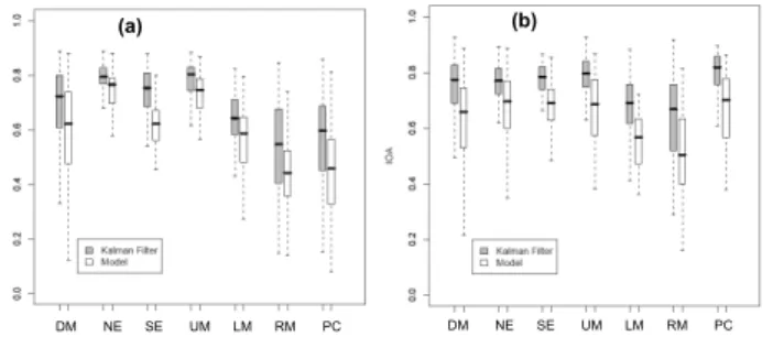
DM NE SE UM LM RM PC
(a)
DM NE SE UM LM RM PC
(b)
Fig. 9.Box plots of index of agreement (IOA) of daily mean PM2.5
(µg/m3)for the raw model (MOD) forecasts and KF bias-adjusted forecasts over the domain (DM) and across all sub-regions during
(a)warm season and(b)cool season.
RMSE (µg/m
3)
RMSE RMSEs RMSEu
Fig. 10. Box plots of RMSE and decomposed RMSE (systematic,
RMSEs; unsystematic, RMSEu) values of the daily mean PM2.5
concentrations (µg/m3)for the raw model forecasts and KF bias-adjusted forecasts.
observed PM2.5 concentrations were larger than 10 µg/m3, the RMSE values associated with KF forecasts were much smaller in both the mean values and the distributions com-pared to the raw model forecasts. In contrast, during the cool season (Fig. 11b), the KF forecasts performed better than the raw model forecasts across all the concentration bins. Ex-amination of the MB distributions over the observed con-centration bins (Fig. 11c and d) reveals that the raw model over-predicted at lower concentrations and under-predicted at higher concentrations, which is similar to the raw model performance for O3forecasts (Kang et al., 2008). The under-prediction at higher concentration bins for PM2.5 forecasts during the warm season was more severe than that during the cool season. In general, the KF forecasts were able to adjust the MB towards zero over all the concentration bins for both seasons.
3.4 Categorical performance
It is equally important to evaluate the performance of an air quality forecast system using the categorical metrics, be-cause for the general public, it is more important to know if
(a) (b)
(d) (c)
Observed Daily Mean PM2.5(µg/m3) Bins
MB
(µ
g/m
3)
RMSE (µg/m
3)
KF Model
0
10
20
30
40
0
10
20
30
40
<5 5-10 10-20 20-30 >=30 <5 5-10 10-20 20-30 >=30
<5 5-10 10-20 20-30 >=30 <5 5-10 10-20 20-30 >=30
-40
-20
-10
0
10
20
-30
-40
-20
0
20
40
Fig. 11.(aandb) RMSE and (candd) mean bias (MB) values over
observed daily mean PM2.5concentration (µg/m3)bins for the raw
model forecasts and the KF bias-adjusted forecasts. The sample sizes for each bin from small to large are 28203, 17526, 19855, 6855, 2716 (Warm Season) and 34072, 36402, 30697, 6771, 2502 (Cool Season).
the NAQFC system could simulate the occurrences of an ex-ceedance or non-exex-ceedance. Categorical evaluations for O3 forecasts have been extensively performed in the past (Kang et al., 2005; Eder et al., 2006, 2009), but similar assessments for PM2.5 forecasts have been limited. Figure 12 displays the false alarm ratio (FAR; also known as probability of false alarm) and hit rate (H; also known as probability of detec-tion) (see Kang et al., 2005; Barnes et al., 2009) for the raw model and KF bias-adjusted daily mean PM2.5forecasts for each of the sub-regions during both the warm and cool sea-sons. An exceedance threshold value of 35 µg/m3for the 24-h mean PM2.5, based on the US National Ambient Air Qual-ity Standard (NAAQS) for PM2.5is used. As seen in Fig. 12, the FAR values associated with the raw model forecasts were similar (∼85%) for both seasons over the entire domain, but
Cool Season
0 20 40 60 80 100
DM NE SE UM LM RM PC
Region
Ra
te
(
%
)
FAR-MOD FAR-KF H-MOD H-KF
Warm Season
0 20 40 60 80 100
DM NE SE UM LM RM PC
Region
R
a
te
(%
)
FAR-MOD FAR-KF H-MOD H-KF
(a)
(b)
Fig. 12.False alarm ratio (FAR) and hit rate (H) for the daily mean
PM2.5forecasts by the raw model and the KF bias-adjustment over the domain (DM) and all the sub-regions during(a)warm season and(b) cool season: FAR-MD, FAR associated with raw model forecasts; FAR-KF, FAR associated with KF forecasts; H-MD, H associated with raw model forecasts; and H-KF, H associated with KF forecasts.
4 Summary
The Kalman filter bias-adjustment technique has been ap-plied to post-process raw PM2.5 air quality forecasts over the continental US domain during the year of 2007 at hourly PM2.5monitoring sites. Though the application and analysis were conducted on archived PM2.5 model forecast output, the methodology is easily adopted for real-time applications. To facilitate performance evaluation, the continental US por-tion of the domain was divided into six sub-regions and the year was split into a cool season and a warm season to exam-ine spatial and seasonal characteristics of the performance of the method. The evaluation of raw model performance sug-gests that the daily mean PM2.5concentrations were gener-ally over-predicted over the eastern part of the domain during the cool season and under-predicted during the warm sea-son; in contrast, the opposite is true for the western part of the domain, i.e., the daily mean PM2.5concentrations were typically under-predicted along the Pacific Coast during the cool season and over-predicted during the warm season; the Rocky Mountain region is an exception where the daily mean PM2.5concentrations were over-predicted through the year.
The KF bias-adjustment technique significantly improved the PM2.5forecasts for locations with hourly PM2.5monitors as revealed by reductions in errors and biases, and higher
correlation coefficients throughout the year and across the entire model domain. The analysis also shows that the KF bias adjustment can quickly respond to transitions from one regime to another during the transition of seasons or model changes.
Analysis of RMSE and MB as a function of observed concentrations suggests that the KF method significantly re-duces the raw model error and bias across all concentration ranges except at lower concentration bins during the warm season. However, the significant reductions in error and bias at the moderate-high concentration ranges helps improve the ability to predict exceedances, a feature desirable for air quality forecasting. The effectiveness and benefits of bias-adjustment of PM2.5model forecasts is also reflected in the categorical evaluations; the KF bias-adjustment technique improved the categorical evaluation metrics significantly by reducing the false alarm ratio and increasing the hit rate for almost all the regions during both the cool and warm seasons. It should be pointed out that the performance of bias-adjusted forecasts is dependent on the performance of the raw model to which the bias-adjustment technique is applied. Because of the complexity in PM2.5composition, formation, and distribution, it is even more critical for the raw model to provide a stable and well-behaved basis to make bias-adjusted forecasts more reliable. This bias-bias-adjusted forecast study was based on the total mass of PM2.5. If the com-ponents of PM2.5 could be bias-adjusted separately, the re-sults may be further improved than those derived from the bias-adjustment of the total PM2.5 mass performed in this study. However, the lack of real-time measurements of spe-ciated PM2.5 hampers the use of KF adjustments on indi-vidual species. Improvements in the representation of fine particulate matter emissions as well as physical and chem-ical processes regulating sources and sinks in atmospheric models are expected as a result of on-going research over the next several years. Nevertheless, our analysis indicates that despite the current uncertainties in the representation of atmospheric processes dictating the distribution of ambient PM2.5, the KF bias-adjustment techniques can be used to im-prove the reliability of short term PM2.5forecasts from such models and, consequently, help in issuance of air-quality-degradation-related health advisories.
Acknowledgements. The authors are grateful to Brian Eder for his constructive and insightful comments on initial drafts of this manuscript. We thank Drs. Luca Delle Monache and Roland B. Stull for providing their original Kalman filter codes. The United States Environmental Protection Agency through its Office of Research and Development funded and managed the research described here. It has been subjected to Agency’s administrative review and approved for publication.
Edited by: D. Lunt
References
Appel, K. W., Bhave, P. V., Gilliland, A. B., Sarwar, G., and Roselle, S. J.: Evaluation of the community multiscale air quality (CMAQ) model version 4.5: Sensitivities impacting model per-formance; Part II-particulate matter, Atmos. Environ., 42, 6057– 6066, doi:10.1016/j.atmosenv.2008.03.036, 2008.
Barnes, L. R., Schultz, D. M., Gruntfest, E. C., Hayden, M. H., and Benight, C. C.: Corrigendum: False Alarm Rate or False Alarm Ratio, Weather Forecast., 24, 1452–1454, doi:10.1175/2009WAF2222300.1, 2009.
Black, T.: The new NMC mesoscale Eta Model: Description and forecast examples, Weather Forecast., 9, 265–278, 1994. Byun, D. W. and Schere, K. L.: Review of the governing equations,
computational algorithms, and other components of the Models-3 Community Multiscale Air Quality (CMAQ) modeling system, Appl. Mech. Rev., 59, 51–77, 2006.
Delle Monache, L., Nipen, T., Deng, X., Zhou, Y., and Stull, R.: Ozone ensemble forecasts: 2. A Kalman filter predictor bias correction, J. Geophys. Res., 111, D05308, doi:10.1029/2005JD006311, 2006.
Delle Monache, L., Wilczak, J., Mckeen, S., Grell, G., Pagowski, M., Peckham, S., Stull, R., McHenry, J., and McQueen, J.: A Kalman-filter bias correction method applied to determin-istic, ensemble averaged, and probabilistic forecasts of sur-face ozone, Tellus Ser. B, 60, 238–249, doi:10.111/j.1600-0889.2007.00332.x, 2008.
Donahue, N. M., Robinson, A. L., and Pandis, S. N.: Atmospheric particulate matter: from smoke to secondary organic aerosol, At-mos. Environ., 43, 94–106, doi:10.1016/j.atmosenv.2008.09.055, 2009.
Eder, B., Davis, J., and Bloomfield, P.: A characterization of the spatiotemporal variation of non-urban ozone in the eastern United States, Atmos. Environ., 27A, 2645–2668, 1993. Eder, B., Kang, D., Mathur, R., Yu, S., and Schere, K.: An
oper-ational evaluation of the Eta-CMAQ air quality forecast model, Atmos. Environ., 40, 4894–4905, 2006.
Eder, B., Kang, D., Mathur, R., Pleim, J., Yu, S., Otte, T., and Pouliot, G.: A performance evaluation of the national air qual-ity forecast capabilqual-ity for the summer of 2007, Atmos. Environ., 43, 2312–2320, doi:10.1016/j.atmosenv.2009.01.033, 2009. Eatough, D. J., Long, R. W., Modey, W. K., and Eatough, N. L.:
Semi-volatile secondary organic aerosol in urban atmospheres: meeting a measurement challenge, Atmos. Environ., 37, 1277– 1292, doi:10.1016/S1352-2130(02)01020-8, 2003.
Gego, E. L., Porter, P. S., Irwin, J. S., Hogrefe, C., and Rao, S. T.: Assessing the comparability of ammonium, ni-trate and sulfate concentrations measured by three air quality monitoring networks, Pure Appl. Geophys., 162, 1919–1939, doi:10.1007/s00024-005-2698-3, 2005.
Glahn, H. R. and Lowry, D. A.: The use of model output statistics (MOS) in objective weather forecasting, J. Appl. Meteor., 11, 1203–1211, 1972.
Grover, B. D., Kleinman, M., Eatough, N. L., Eatough, D. J., Hopke, P. K., Long, R. W., Wilson, W. E., Meyer, M. B., and Ambs, J. L.: Measurement of total PM2.5 mass (nonvolatile
plus semivolatile) with the Filter Dynamic Measurement System tapered element oscillating microbalance monitor, J. Geophys. Res., 110, D07S03, doi:10.1029/2004JD004995, 2005. Kalman, R. E.: A new approach to linear filtering and prediction
problems, J. Basic Eng., 82, 35–45, 1960.
Kang, D., Mathur, R., Rao, S. T., and Yu, S.: Bias adjustment tech-niques for improving ozone air quality forecasts, J. Geophys. Res., 113, D23308, doi:10.1029/2008JD010151, 2008.
Kang, D., Eder, B. K., Stein, A. F., Grell, G. A., Peckham, S. E., and McHenry, J.: The New England air quality forecasting pilot pro-gram: Development of an evaluation protocol and performance benchmark, J. Air Waste Manage. Assoc., 55, 1782–1796, 2005. Mathur, R., Yu, S., Kang, D., and Schere, K. L.: Assess-ment of the wintertime performance of developAssess-mental partic-ulate matter forecasts with the Eta-Community Multiscale Air Quality modeling system, J. Geophys. Res., 113, D02303, doi:10.1029/2007JD008580, 2008.
McHenry, J. N., Ryan, W. F., Seaman, N. L., Coats Jr., C. J., Pudykiewicz, J., Arunachalam, S., and Vukovich, J. M.: A real-time Eulerian photochemical model forecast system: Overview and initial ozone forecast performance in the northeast U. S. cor-ridor, B. Am. Meteorol. Soc., 85, 525–548, 2004.
McKeen, S., Wilczak, J., Grell, G., et al.: Assessment of an ensem-ble of seven real-time ozone forecasts over eastern North Amer-ica during the summer of 2004, J. Geophys. Res., 110, D21307, doi:10.1029/2005JD005858, 2005.
McKeen, S., Chung, S. H., Wilczak, J., et al.: Evaluation of several PM2.5 forecast models using data collected during the ICARTT/NEAQS 2004 field study, J. Geophys. Res., 112, D10S20, doi:10.1029/2006JD007608, 2007.
McMurry, P. A.: A review of atmospheric aerosol measurements, Atmos. Environ., 34, 1959–1999, 2000.
National Research Council: Research Priorities for Particulate Mat-ter 1: Immediate Priorities and a Long-Range Research Portfolio, Natl. Acad. Press, Washington, D.C., 1998.
Otte, T. L., Pouliot, G., Pleim, J. E., et al.: Linking the Eta Model with the Community Multiscale Air Quality (CMAQ) modeling system to build a national air quality forecasting system, Weather Forecast., 20, 367–384, 2005.
Schwede, D., Pouliot, G., and Pierce, T.: Changes to the Biogenic Emissions Inventory System Version 3 (BEIS3) at the 4th Annual CMAS Models-3 User’s Conference, 26–28 September 2005, Chapel Hill, NC, USA, 2005.
Wilczak, J., McKeen, S., Djalalova, I., Grell, G., Peckham, S., Gong, W., Bouchet, V., Moffet, R., McHenry, J., Lee, P., Tang, Y., and Carmichael, G. R.: Bias-corrected ensemble and proba-bilistic forecasts of surface ozone over eastern North America during the summer of 2004, J. Geophys. Res., 111, D23S28, doi:10.1029/2006JD007598, 2006.
Willmott, C. J.: On the validation of models, Phys. Geogr., 2, 184– 194, 1981.