The ASSET intercomparison of ozone analyses: method and first results

(1)

ACPD

6, 4495–4577, 2006

Intercomparison of ozone analyses

A. J. Geer et al.

Title Page

Abstract Introduction

Conclusions References

Tables Figures

◭ ◮

Back Close

Full Screen / Esc

Printer-friendly Version

Interactive Discussion

EGU

Atmos. Chem. Phys. Discuss., 6, 4495–4577, 2006 www.atmos-chem-phys-discuss.net/6/4495/2006/ © Author(s) 2006. This work is licensed

under a Creative Commons License.

Atmospheric Chemistry and Physics Discussions

The ASSET intercomparison of ozone

analyses: method and first results

A. J. Geer1, W. A. Lahoz1, S. Bekki2, N. Bormann3, Q. Errera4, H. J. Eskes5,

D. Fonteyn4, D. R. Jackson6, M. N. Juckes7, S. Massart8, V.-H. Peuch9,

S. Rharmili2, and A. Segers5

1

Data Assimilation Research Centre, University of Reading, Reading, UK

2

CNRS Service Aeronomie, Universit ´e Pierre et Marie Curie, Paris, France

3

European Centre for Medium-Range Weather Forecasts, Reading, UK

4

Institut d’A ´eronomie Spatiale de Belgique, Brussels, Belgium

5

Royal Netherlands Meteorological Institute, De Bilt, The Netherlands

6

Met Office, Exeter, UK

7

British Atmospheric Data Centre, Rutherford Appleton Laboratory, Chilton, nr Didcot, UK

8

CERFACS, Toulouse, France

9

CNRM-GAME, M ´et ´eo-France and CNRS URA 1357, Toulouse, France

Received: 6 February 2006 – Accepted: 7 March 2006 – Published: 7 June 2006

(2)

ACPD

6, 4495–4577, 2006

A. J. Geer et al.

Title Page

Tables Figures

◭ ◮

Back Close

Full Screen / Esc

EGU

Abstract

This paper examines 11 sets of ozone analyses from 7 different data assimilation

sys-tems. Two are numerical weather prediction (NWP) systems based on general circu-lation models (GCMs); the other five use chemistry transport models (CTMs). These systems contain either linearised or detailed ozone chemistry, or no chemistry at all. 5

In most analyses, MIPAS (Michelson Interferometer for Passive Atmospheric Sound-ing) ozone data are assimilated. Two examples assimilate SCIAMACHY (Scanning Imaging Absorption Spectrometer for Atmospheric Chartography) observations. The analyses are compared to independent ozone observations covering the troposphere, stratosphere and lower mesosphere during the period July to November 2003.

10

Through most of the stratosphere (50 hPa to 1 hPa), biases are usually within±10%

and standard deviations less than 10% compared to ozonesondes and HALOE (Halo-gen Occultation Experiment). Biases and standard deviations are larger in the upper-troposphere/lower-stratosphere, in the troposphere, the mesosphere, and the Antarctic ozone hole region. In these regions, some analyses do substantially better than oth-15

ers, and this is mostly due to differences in the models. At the tropical tropopause,

many analyses show positive biases and excessive structure in the ozone fields, likely due to known deficiencies in assimilated tropical wind fields and a degradation in MI-PAS data at these levels. In the southern hemisphere ozone hole, only the analyses which correctly model heterogeneous ozone depletion are able to reproduce the near-20

complete ozone destruction over the pole. In the upper-stratosphere and mesosphere (above 5 hPa), some ozone photochemistry schemes caused large but easily remedied biases. The diurnal cycle of ozone in the mesosphere is not captured, except by the one system that includes a detailed treatment of mesospheric chemistry.

In general, similarly good results are obtained no matter what the assimilation 25

(3)

ACPD

6, 4495–4577, 2006

A. J. Geer et al.

Title Page

Tables Figures

◭ ◮

Back Close

Full Screen / Esc

EGU

almost as good as the MIPAS analyses; analyses based on SCIAMACHY limb profiles are worse in some areas, due to problems in the SCIAMACHY retrievals.

Using the analyses as a transfer standard, and treating MIPAS observations as point

retrievals, it is seen that MIPAS is∼5% higher than HALOE in the mid and upper

strato-sphere and mesostrato-sphere (above 30 hPa), and of order 10% higher than ozonesonde 5

and HALOE in the lower stratosphere (100 hPa to 30 hPa).

1 Introduction

The Assimilation of ENVISAT Data (ASSET,http://darc.nerc.ac.uk/asset) project aims

to provide analyses of atmospheric chemical constituents, based on the assimilation of observations from the ENVISAT satellite, and to develop chemical weather and UV 10

forecasting capabilities. Data are assimilated into a variety of different systems, includ-ing chemical transport models (CTMs) with detailed chemistry or simple chemistry, and Numerical Weather Prediction (NWP) systems based on General Circulation Models (GCMs), either with simple chemistry, or coupled to detailed-chemistry CTMs. Data

as-similation techniques (see e.g.,Kalnay,2003) include three and four-dimensional

vari-15

ational data assimilation (3D-Var and 4D-Var) and the Kalman Filter (KF). It is hoped that, by confronting these various models and techniques with the newly available EN-VISAT observations, it will be possible both to gain an understanding of their strengths and weaknesses, and to make new developments. A number of ozone analyses have been created within the ASSET project; this paper compares them to independent ob-20

servations and to ozone analyses from outside the project. There have been a number

of previous intercomparisons between the ozone distributions in different CTMs (e.g.,

Bregman et al.,2001;Roelofs et al.,2003) but this is the first time ozone analyses have been compared.

Datasets of assimilated ozone will be useful for research and monitoring of ozone 25

depletion (e.g.,WMO,2003), tropospheric pollution, and UV fluxes, and beyond this,

(4)

upper-ACPD

6, 4495–4577, 2006

A. J. Geer et al.

Title Page

Tables Figures

◭ ◮

Back Close

Full Screen / Esc

EGU

troposphere/lower-stratosphere (UTLS), ozone has a photochemical relaxation time of order 100 days, and it can be used as a tracer to infer atmospheric motions using 4D-Var (e.g.,Riishøjgaard,1996;Peuch et al.,2000). Second, NWP systems have typically used a zonal mean ozone climatology in modelling heating rates and in the forward radiative transfer calculations used in the assimilation of satellite radiances such as 5

those from the Atmospheric Infrared Sounder (AIRS). An estimate of the true 3-D ozone distribution is likely to improve these calculations. Experiments at ECMWF found that

variations in ozone amounts of∼10 to 20% could result in changes in modelled tropical

UTLS temperatures of up to 4 K (Cariolle and Morcrette, 2006). The diurnal cycle

of ozone is important in the middle atmosphere. Model runs with diurnally varying 10

ozone show temperature di_fferences of up to 3 K in the stratosphere, compared to

those with climatological ozone (Sassi et al., 2005). A prognostic ozone field also

allows the modelling of feedbacks between radiation, chemistry and dynamics, and this is expected to improve forecasts, especially over longer timescales. However, no study has yet found a clear benefit in terms of forecast scores (e.g.,Morcrette,2003). Finally, 15

in order to simulate a good ozone distribution, models used in assimilation systems must be able to simulate stratospheric transport well; problems are often revealed when these models are confronted with real observations (e.g.,Geer et al.,2006).

Different approaches can be used for ozone data assimilation and the choice will vary depending on the application. Chemical transport models typically use operationally-20

produced analyses of wind and temperature (such as those from ECMWF) to advect chemical constituents. If chemistry is treated approximately, these models are ex-tremely fast and can be used to assimilate many months of observations in a few days on a desktop computer. Including a detailed chemistry scheme, with dozens of con-stituents and hundreds of reactions, allows a more accurate simulation of the ozone 25

distribution, but is slower. The CTM approach has been very popular for ozone analy-sis systems (e.g.,Fisher and Lary,1995;Khattatov et al.,2000;Elbern and Schmidt,

2001;Errera and Fonteyn,2001;Stajner et al.˘ , 2001; Chipperfield et al., 2002; Fierli

(5)

ACPD

6, 4495–4577, 2006

A. J. Geer et al.

Title Page

Tables Figures

◭ ◮

Back Close

Full Screen / Esc

EGU

Massart et al.,2005;Segers et al.,2005a;Wargan et al.,2005). It is also possible to

introduce a prognostic ozone field directly into an NWP system (e.g.,Struthers et al.,

2002;Dethof and H ´olm,2004;Geer et al.,2006), but ozone assimilation then becomes part of a very large operational system, requiring a supercomputer. Much work is still required to confirm the proposed benefits of including ozone directly into NWP systems. 5

One alternative approach is to couple CTMs, with a detailed description of chemistry, to GCM-based NWP systems, such that feedbacks between chemistry, dynamics and radiation can be maintained.

Current operational satellite ozone observations include the Total Ozone Mapping Spectrometer (TOMS), measuring total column ozone, and the Solar Backscatter Ul-10

traviolet (SBUV) instrument (e.g.,Bhartia et al.,1996), which produces vertical profiles. ENVISAT, launched in 2002, provides the instruments MIPAS (Michelson Interferom-eter for Passive Atmospheric Sounding), SCIAMACHY (Scanning Imaging Absorption Spectrometer for Atmospheric Chartography) and GOMOS (Global Ozone Monitoring by Occultation of Stars). Between them, these instruments measure many species be-15

yond ozone, and vertical resolution is much improved over the operational instruments. For example, MIPAS has roughly twice the vertical resolution of SBUV in the

strato-sphere (see e.g. Fig. 2, Wargan et al., 2005). The ASSET project is based around

assimilating the data from ENVISAT. The EOS-Aura satellite, launched in 2004, has in-struments with similar capabilities. Research inin-struments such as those on ENVISAT 20

and Aura do, however, have a limited lifetime and data products are not always available quickly enough to be included in operational NWP schedules. Hence research satellite data is often best used for re-analyses, and to help improve models and assimilation systems such that the operational observations, such as SBUV, may be assimilated more successfully.

25

For this intercomparison, ozone analyses have been made for the period July to November 2003, chosen because of the availability of good quality MIPAS data. This

period included one of the largest ozone holes on record (e.g.,Dethof,2003a), caused

(6)

ACPD

6, 4495–4577, 2006

A. J. Geer et al.

Title Page

Tables Figures

◭ ◮

Back Close

Full Screen / Esc

EGU

which was destroyed by the usual top-down break-up during October and November (Lahoz et al.,2006).

Eleven analysis runs are included in the intercomparison, made using seven different

systems, summarised in Table1. Two climatology-derived products are also included in

the intercomparison. All but two analysis runs assimilate MIPAS ozone data; the others 5

assimilate SCIAMACHY. Both CTMs and GCMs are represented, and ozone chemistry may or may not be modelled. If included, it is done either by highly detailed reaction

schemes or via a parametrization often known as a Cariolle scheme (e.g.,Cariolle and

D ´equ ´e,1986;McLinden et al.,2000;McCormack et al.,2004). The Cariolle scheme is a linearisation of ozone photochemistry around an equilibrium state, using parameters 10

derived from a more detailed model.

Most of the analysis systems are focused on the stratosphere, but the scope of the comparison spans from the troposphere to the mesosphere. Analyses are interpolated from their native resolution onto a common grid and then compared to independent ozone data from Halogen Occultation Experiment (HALOE), ozonesondes and TOMS, 15

and to MIPAS. Most data, figures, and code are being made publicly available via the project website (http://darc.nerc.ac.uk/asset).

This paper introduces the intercomparison project, the method used, the indepen-dent data sources, and the analysis systems involved. It outlines many of the initial results, such as problems found with some implementations of linearised ozone chem-20

istry schemes, and it draws initial conclusions on the various different methods used.

There is not scope in this paper for detailed comparisons, such as between different

types of chemistry schemes, or between 3D-Var and 4D-Var. These are anyway best performed in an experimental setting within a single assimilation system. However, the intercomparison provides a framework under which these results, and their signif-25

(7)

ACPD

6, 4495–4577, 2006

A. J. Geer et al.

Title Page

Tables Figures

◭ ◮

Back Close

Full Screen / Esc

EGU

2 Analyses

Before describing in detail the analyses and climatologies in the intercomparison, we

show examples of the ozone fields at 68 hPa on 31 August 2003 (Fig.1). Sunlight has

started to return to high latitudes after the winter, triggering the depletion of ozone in a

ring around the pole (see e.g.,WMO,2003). Sunlight has not yet returned to the pole

5

itself. The ring of higher ozone (3 to 5 ppmm) at about 45◦S is the remainder of ozone

that has descended throughout the SH high latitudes during the winter, from levels higher in the atmosphere where ozone amounts are greater. It is clear that at 68 hPa

all the analyses show broadly similar and (from Sect.5) realistic structures. Compared

to the others, the KNMI SCIAMACHY profile analyses have a bias; due to a lack of 10

observations before October they are based principally on the free-running model.

2.1 ECMWF

Ozone observations have been assimilated into the operational ECMWF analyses (http://www.ecmwf.int) since April 2002. During 2003, GOME columns and SBUV pro-files were assimilated, though in August and September 2003, there was very limited 15

availability of GOME data. MIPAS was assimilated operationally from from 7 October 2003 until 25 March 2004. Here we consider two datasets: (a) the operational analyses and (b) a dataset that includes assimilated MIPAS ozone throughout the July-November period, based on a pre-operational test suite before 7th October, and operational data

after 7 October (Dethof, 2003a). In all cases, the MIPAS data is version 4.59 of the

20

Near Real Time product. Gross outliers in the MIPAS retrievals are rejected based on a comparison against the background ozone. Variational quality control is also applied (Andersson and J ¨arvinen,1999).

The GCM in use when the analyses were made had a horizontal resolution of T511

(∼50 km) and 60 levels in the vertical, from the surface up to 0.1 hPa. Ozone was

ad-25

(8)

ACPD

6, 4495–4577, 2006

A. J. Geer et al.

Title Page

Tables Figures

◭ ◮

Back Close

Full Screen / Esc

EGU

2004), which includes a description of heterogeneous ozone depletion. Climatological

ozone (Fortuin and Langematz,1995), not prognostic ozone, was used for modelling

heating rates.

Data assimilation uses 4D-Var (e.g.,Rabier et al.,2000). Ozone is assimilated

uni-variately, but it can still affect the dynamical analyses through the 4D-Var method (e.g., 5

Riishøjgaard,1996) and through the influence of ozone on the assimilation of temper-ature radiances. Background error correlations are calculated using an ensemble of

analyses (Fisher,2003); background error variances are flow dependent.

2.2 DARC/Met Office

The Met Office NWP system has recently been extended to allow the assimilation

10

of ozone (Jackson and Saunders, 2002; Jackson, 2004) but ozone is not

assimi-lated operationally. Here, MIPAS v4.61 ozone and temperature are assimiassimi-lated in re-analysis mode, alongside all operational dynamical observations, using a strato-sphere/troposphere version of the operational NWP system. The system is that

de-scribed in Geer et al. (2006), but with a number of improvements to the GCM and

15

no assimilation of HIRS (High resolution infrared radiation sounder) channel 9 ozone radiances.

The assimilating GCM has a horizontal resolution of 3.75◦ _{longitude by 2.5}◦ _latitude

and 50 levels in the vertical, from the surface to∼0.1 hPa. It uses a new dynamical

core (Davies et al.,2005) which includes a semi-Lagrangian transport scheme. This

20

gives a better description of the Brewer-Dobson circulation than that seen in Geer

et al. (2006). Ozone photochemistry is parametrized by v1.0 of theCariolle and D ´equ ´e

(1986) scheme. Improving on Geer et al.(2006), heterogeneous ozone chemistry is

now parametrized, using a cold tracer scheme (Eskes et al., 2003). Climatological

ozone (Li and Shine, 1995), not the prognostic field, is used for modelling heating

25

rates.

Data assimilation uses 3D-Var (Lorenc et al.,2000). As for ECMWF, ozone is

(9)

ACPD

6, 4495–4577, 2006

A. J. Geer et al.

Title Page

Tables Figures

◭ ◮

Back Close

Full Screen / Esc

EGU

of ozone on the dynamical analysis is through its influence on temperature radiance assimilation. Background error covariances are uniform for all latitudes and longitudes,

and they are based on the ECMWF vertical covariances. As illustrated inGeer et al.

(2006), the MIPAS ozone observations are subject to quality control, but with a lax

threshold, so very few observations are rejected. 5

2.3 KNMI

The Royal Netherlands Meteorological Institute (KNMI) operate a CTM which has been used to assimilate SCIAMACHY ozone data. The CTM uses a subset of 44 of the

ECMWF model levels, from the surface to 0.1 hPa, on a 3◦ _{longitude by 2}◦ _latitude

grid. Data assimilation is done using a sub-optimal Kalman Filter (see e.g.,Kalnay,

10

2003), where the background error variances, but not the correlations, are advected as

a tracer. Two di_fferent configurations are presented.

The first configuration assimilates total column ozone from SCIAMACHY, retrieved at KNMI using the TOSOMI algorithm (Total Ozone retrieval scheme for SCIAMACHY

based on the OMI DOAS algorithm, Eskes et al., 2005b). The CTM is driven by

15

ECMWF operational analyses of winds and temperatures. Ozone photochemistry is

parametrized using the LINOZ scheme (McLinden et al.,2000), a variant on Cariolle

and D ´equ ´e (1986). Heterogeneous chemistry uses a cold tracer scheme. For

assim-ilating total column observations, the vertical error correlations are set proportional to

the vertical ozone profile. The system is very similar to that described inEskes et al.

20

(2003).

The second configuration assimilates ozone profiles (IFE v1.6) from the limb-sounding mode of SCIAMACHY into the TM5 model. SCIAMACHY limb profiles are mainly available for October and November 2003; July to September is a free model run apart from a few assimilated profiles in August. The main uncertainty in the SCIA-25

MACHY product is pointing, which has a vertical offset of 1–2 km (Segers et al.,2005b). All profiles have been shifted in the vertical to get the best match with model forecasts

(10)

ACPD

6, 4495–4577, 2006

A. J. Geer et al.

Title Page

Tables Figures

◭ ◮

Back Close

Full Screen / Esc

EGU

v1.0 and a cold-tracer scheme. The CTM is driven by ECMWF short range forecasts

at 3 hourly intervals. The system is otherwise similar to that described inSegers et al.

(2005a).

2.4 BASCOE

The Belgian Assimilation System of Chemical Observations from ENVISAT (BASCOE, 5

http://www.bascoe.oma.be) is a 4D-Var assimilation system descended from that

de-scribed in Errera and Fonteyn (2001). Studies of the Antarctic and Arctic winter

using the CTM of BASCOE can be found in Chabrillat et al. (2006)1 and Daerden

et al. (2006)2. MIPAS v4.61 ozone (O3), water vapour (H2O), nitric acid (HNO3), nitric

dioxide (NO2), methane (CH4) and nitrous oxide (N2O) are assimilated. Observations

10

are subjected to an Optimal Interpolation Quality Check (OIQC, e.g. Gauthier et al.,

2003). In practice, the lowest MIPAS ozone observations in the ozone hole are rejected.

Observations are also rejected if they fail a check for spurious vertical oscillations in the profile.

The model includes 57 chemical species and 4 types of stratospheric PSC parti-15

cles (ice; supercooled ternary solution, STS; nitric acid trihydrate, NAT; sulphuric acid tetrahydrate, SAT) with a full description of stratospheric chemistry and microphysics of PSCs. All chemical species are advected and interact through 143 gas-phase reac-tions, 48 photolysis reactions and 9 heterogeneous reactions. To allow for calculating transport of PSCs, size distributions of each type are discretized using 36 bins from 20

0.002 to 36 µm. PSC microphysics is described by the PSCBox scheme (Larsen et al.,

1

Chabrillat, S. H., Van Roozendael, M., Daerden, F., Errera, Q., Hendrick, F., Bonjean, S., Wilms-Grabe, W., Wagner, T., Richter, A., and Fonteyn, D.: Quantitative assessment of 3-D PSC-chemistry-transport models by simulation of GOME observations during the Antarctic winter of 2002, in preparation, 2006.

2

(11)

ACPD

6, 4495–4577, 2006

A. J. Geer et al.

Title Page

Tables Figures

◭ ◮

Back Close

Full Screen / Esc

EGU

2000). In order to improve agreement with MIPAS ozone, O₂ photolysis rates were

multipled by 1.25. This version is referred to as v3d24.

Based on early results of this intercomparison, a new version of BASCOE, v3q33, was produced. Among the changes, v3q33 replaces the full PSC calculation by a parametrization that defines (1) surface area density of ice and NAT when their occur-5

rence is possible and (2) the loss of HNO3 and H2O due to sedimentation (Chabrillat

et al., 20061). Ice PSCs are supposed to exist in the winter/spring polar regions at

any grid point where the temperature is colder than 186 K, and NAT PSCs at any grid point where the temperature is colder than 194 K. The surface area density is set to 10−6_cm2_/_cm3_{in the first case and 10}−7_cm2_/cm3_{in the second. Additionally in v3q33,}

10

O2 photolysis rates are no longer scaled; this reduces the bias against HALOE but

increases it against MIPAS (see Sect.5.1). Finally, the Arakawa A grid of v3d24 was

replaced by a C grid (see e.g.,Kalnay,2003) in v3q33.

The CTM is driven by ECMWF operational analyses of winds and temperatures, and

uses a subset of 37 of the ECMWF model levels, from the surface to 0.1 hPa, on a 5◦

15

longitude by 3.75◦latitude grid.

Data assimilation is done using 4D-Var. The background error standard deviation is

set as 20% of the background ozone amount. Though there are no off-diagonal

ele-ments in the background error covariances (i.e. no vertical or horizontal correlations), information from MIPAS observations is still spread through the observation operator, 20

as in other systems. Here, it averages the 8 grid points surrounding the measurement point, and the relatively broad horizontal resolution of the grid also helps to spread the information.

2.5 M ´et ´eo-France/CERFACS

The M ´et ´eo-France/CERFACS assimilation system is based upon the 3-D CTM 25

MOCAGE and the PALM software (Massart et al., 2005). MIPAS v4.61 ozone data

are assimilated, but not beyond 80◦of latitude.

(12)

sophisti-ACPD

6, 4495–4577, 2006

A. J. Geer et al.

Title Page

Tables Figures

◭ ◮

Back Close

Full Screen / Esc

EGU

cation (for instance, the number of chemical tracers involved, the physical or chemi-cal parametrizations, the horizontal and vertichemi-cal geometries) and the data assimilation technique can be changed easily; this makes the MOCAGE-PALM system a useful platform for sensitivity studies in chemical data assimilation.

MOCAGE is a flexible tropospheric and stratospheric 3-D CTM developed at M ´et ´eo-5

France, offering several configurations of varying computational costs. Two separate

configurations are examined here. The first uses linear ozone chemistry, with v2.1 of theCariolle and D ´equ ´e(1986) scheme. The second includes a detailed representation of stratospheric and upper tropospheric chemistry, based upon the REPROBUS

chem-ical scheme (Lef `evre et al., 1994), which comprises 55 transients and species and

10

takes into account heterogeneous chemistry on polar stratospheric clouds (Carslaw

et al., 1995; Lef `evre et al., 1998). The REPROBUS chemistry version of MOCAGE

has already been used for UTLS assimilation studies (Cathala et al.,2003). A more

comprehensive version of MOCAGE, with comprehensive tropospheric chemistry, is run daily in operational mode at M ´et ´eo-France for chemical weather and air quality ap-15

plications (Dufour et al.,2004, see daily global forecasts athttp://www.prevair.org/en)

MOCAGE relies on a semi-Lagrangian advection scheme (Josse et al.,2004). For

the experiments presented here, MOCAGE has a 2◦ by 2◦ horizontal resolution and

47 hybrid sigma/pressure levels extending from the surface up to 5 hPa. The meteo-rological forcings are M ´et ´eo-France ARPEGE operational meteometeo-rological analyses of 20

pressure, winds, temperature and humidity (Courtier et al.,1991), available every 6 h. Any assimilation algorithm can be seen as a sequence of elementary operations

or elementary components that can exchange data (Lagarde et al.,2001). Based on

this idea, the CERFACS PALM software (http://www.cerfacs.fr/∼_palm_{) manages the}

dy-namic launching of the coupled components (forecast model, algebra operators, I/O of 25

observational data) and the parallel data exchanges. The MOCAGE-PALM assimila-tion system is set up here in a 3D-FGAT configuraassimila-tion (3-D First Guess at Assimilaassimila-tion

Time,Fisher and Andersson,2001). As a first approximation, background error

(13)

ACPD

6, 4495–4577, 2006

A. J. Geer et al.

Title Page

Tables Figures

◭ ◮

Back Close

Full Screen / Esc

EGU

spread assimilation increments spatially, horizontal background error correlations are

modelled using a generalized diffusion operator (Weaver and Courtier, 2001), with a

length-scale of 4◦; no vertical background error correlations are considered.

2.6 MIMOSA

MIMOSA (Mod èle Isentrope de transport M éso échelle de l’Ozone Stratosph érique par 5

Advection) is a CTM driven by ECMWF operational winds and temperatures (Fierli

et al.,2002). MIPAS v4.61 ozone data are assimilated. There is no quality control;

all observations are included. There are 16 isentropic levels from 335 K to 1650 K, approximately spanning the stratosphere (∼200 hPa to∼1 hPa) and a 1◦by 1◦

latitude-longitude grid. Advection is semi-Lagrangian. The model includes neither ozone chem-10

istry nor cross-isentropic transport.

Data assimilation is done using a sub-optimal Kalman Filter with advected back-ground error variances, and uses the Physical Space Assimilation System method

(PSAS, e.g. Kalnay, 2003). Background error correlations are flow dependent and

anisotropic, specified in terms of distance and the potential vorticity (PV) field. The 15

model error covariance (Q) is diagonal, and proportional to the ozone amount, x,

e.g.Q=(qx)2whereq=0.024 day−1and has been tuned usingχ2tests.

ECMWF operational temperature and pressure fields are used to interpolate these isentropic analyses onto pressure levels for this study.

2.7 Juckes

20

These are analyses produced by a direct inversion method (Juckes,2005), which

as-similates many months of MIPAS v4.61 ozone data by making a single iterative solu-tion. The physical constraint is based on an isentropic transport equasolu-tion. Rather than discretising the predictive equations (which would give a CTM), the product of these equations with their adjoint is discretised. The resulting self-adjoint system of equa-25

(14)

ACPD

6, 4495–4577, 2006

A. J. Geer et al.

Title Page

Tables Figures

◭ ◮

Back Close

Full Screen / Esc

EGU

Kalman Smoother with fully advected background error covariances.

Ozone transport is driven by ECMWF operational winds and temperatures, on 13 isentropic levels from 380 K to 3000 K. In the horizontal, a binary thinned

latitude-longitude spherical grid is used, giving approximately 2◦ by 2◦ resolution. The model

error covariance (Q) is diagonal, with a constant value of 0.02 ppmv2/day2. The model 5

includes neither ozone chemistry nor cross-isentropic transport. As for MIMOSA,

ECMWF pressure and temperature fields are used for interpolation onto pressure lev-els in this study.

2.8 Climatology

To contrast with the assimilated ozone fields, we include a climatology-derived product 10

in the comparison. As a minimum, we would expect the analyses to do better than

climatology. We combine the Logan (1999) tropospheric ozone climatology with the

Fortuin and Kelder (1998) stratospheric ozone climatology. In each case, the clima-tologies are resolved on a monthly basis.

The Logan (1999) climatology uses ozonesonde, surface in-situ data and the 15

TOMS/Stratospheric Aerosol and Gas Experiment (SAGE) tropospheric residual, to produce a partly 3-D and partly 2-D climatology on 13 levels from 1000 hPa to 100 hPa, covering latitudes from 89◦_{S to 89}◦_{N. The}_{Fortuin and Kelder}₍₁₉₉₈_{) climatology uses}

ozonesondes, SBUV and TOMS total ozone, from 1980 to 1991, to produce a 2-D (latitude-pressure) climatology with 19 levels from 1000 hPa to 0.3 hPa and covering 20

latitudes from 80◦_{S to 80}◦_N.

An ozone field was created on the intercomparison common grid, daily at 00Z and 12Z, by interpolating the climatologies linearly in time, and treating the climatologies as representative of the 15th of each month. Beyond the northern and southern limits of

the climatologies, horizontal extrapolation was done at constant value. Logan (1999)

25

values were taken for levels at 150 hPa and below, and Fortuin and Kelder (1998)

above, up to 0.3 hPa. Figure1shows that this results in a zonal distribution which, as

(15)

ACPD

6, 4495–4577, 2006

A. J. Geer et al.

Title Page

Tables Figures

◭ ◮

Back Close

Full Screen / Esc

EGU

An attempt was made to create a PV-mapped ozone climatology in order to capture synoptic variability in the ozone field, but in comparisons against independent data, it proved no better than the largely zonal mean one described above. The

climatol-ogy derived byRandel et al. (1998), based on Upper Atmosphere Research satellite

(UARS) HALOE and Microwave Limb Sounder (MLS) measurements, is made using 5

equivalent latitude coordinates. This was mapped onto the longitudes, latitudes and times of the intercomparison common grid using ECMWF operational PV fields.

Fig-ure1indicates that this product is able to capture some of the synoptic variations seen

in the analyses, but that the fields are affected by noise in the PV-derived equivalent

latitudes. This is a well-known limitation of PV-derived equivalent latitude (Allen and

10

Nakamura,2003). In addition, in the mid and upper stratosphere where ozone

photo-chemistry is relatively fast, it can quickly remove any relationship between ozone and

PV. See, for example, the filamentation event inLahoz et al.(2006). Hence, we do not

consider the PV-mapped ozone product further in the paper, but it forms part of the set of data and figures available from the website, and it is worth noting the limitations of 15

this approach.

2.9 Comparison of ozone background errors

The background error covariance matrix (e.g.,Kalnay,2003) is important in

determin-ing the weight given to observations in data assimilation. In general, at the observation point, more weight is given to the model as the background error standard deviation 20

becomes smaller compared to the observation error standard deviation. However, the spreading of information away from the observation point is determined by the back-ground error correlations, any observation error correlations (not usually considered), and the observation operator. Here, only the DARC and ECMWF systems include ver-tical correlations in the background errors. The general impact of observations on the 25

(16)

sys-ACPD

6, 4495–4577, 2006

A. J. Geer et al.

Title Page

Tables Figures

◭ ◮

Back Close

Full Screen / Esc

EGU

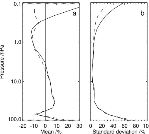
tems, and compare it to the MIPAS ozone observation error standard deviation (Fig.2).

In each case these have been normalised by the climatological ozone amount (see

Sect. 4 for the method). The comparison is done to illustrate the varied approaches

to background error modelling, and to give some indication of the weight assigned to

observations in the different systems. As already noted, however, many other factors

5

affect the observations’ weight in the final analysis.

Figure2shows large differences in the ozone background error standard deviations

assumed in the assimilation systems. In the mid and upper stratosphere (levels above 30 hPa), DARC and ECMWF background error standard deviations are less than 5% of the ozone field, whereas the BASCOE and (to 5 hPa) M ´et ´eo-France/CERFACS sys-10

tems are typically 20%. This suggests the DARC and ECMWF analyses give less weight to observations at these levels. MIPAS observation errors are markedly larger at the tropical tropopause, and all the systems are likely to give relatively lower weight to MIPAS observations here than in the rest of the stratosphere. Work is ongoing to

understand the large differences between systems.

15

3 Ozone observations

3.1 MIPAS

All analyses examined here assimilate MIPAS ozone, except the KNMI analyses, which assimilate SCIAMACHY. Typically, assimilation systems produce observation minus first guess (O-F) statistics that are used for monitoring biases between the observa-20

tions and the models, and checking that statistical assumptions are valid in the assim-ilation algorithm (e.g., Talagrand, 2003;Stajner et al.˘ , 2004). Here, instead of using

the many different formats of O-F produced by individual systems, we simply compare

the common-gridded analysis products to MIPAS, similarly to the way we compare to independent HALOE data.

25

(17)

ACPD

6, 4495–4577, 2006

A. J. Geer et al.

Title Page

Tables Figures

◭ ◮

Back Close

Full Screen / Esc

EGU

limb (Fischer and Oelhaf,1996). MIPAS operational data are available between July

2002 and March 2004, after which instrument problems meant it could only be used on an occasional basis. The operational measurements were made along 17 discrete lines-of-sight in the reverse of the flight direction of ENVISAT, with tangent heights

be-tween 8 km and 68 km. The vertical resolution was∼3 km and the horizontal resolution

5

was∼300 km along the line of sight. ENVISAT follows a sun-synchronous polar orbit,

allowing MIPAS to sample globally, and to produce up to∼1000 atmospheric profiles

per day. Coverage is quite uniform in latitude and time (see Fig.4).

From the infrared spectra, ESA retrieved profiles of pressure, temperature, ozone,

water vapour, HNO₃, NO₂, CH₄ and N₂O at up to 17 tangent points (ESA, 2004).

10

MIPAS version 4.61 data, reprocessed o_ffline, is used throughout this work, except in

the ECMWF assimilation runs, where the Near Real Time v4.59 product was used.

The differences between v4.59 and v4.61 processors are minor.

MIPAS ozone appears unbiased when compared to independent data except in the lower stratosphere where a small positive bias has been noted (Dethof,2003a,b,2004; 15

Fischer and Oelhaf,2004;Wargan et al.,2005;Geer et al.,2006). However, a com-parison against ozonesondes using the MIPAS averaging kernels identified no bias (Migliorini et al., 2004). Using the analyses as a transfer standard, and treating MI-PAS retrievals as point measurements, this intercomparison suggests a positive bias of order 5% in the upper stratosphere with respect to HALOE, increasing to roughly 20

10% with respect to sonde and HALOE in the lower stratosphere. The official MIPAS

validation papers are currently in preparation.

To calculate statistics of (analysis – MIPAS), the analyses are interpolated from the

intercomparison common grid to the MIPAS retrieval points. The paired differences are

then binned to the nearest pressure level on the intercomparison grid. Tests showed 25

(18)

ACPD

6, 4495–4577, 2006

A. J. Geer et al.

Title Page

Tables Figures

◭ ◮

Back Close

Full Screen / Esc

EGU

The statistics are based on a set of MIPAS observations including all those supplied in the ESA data files, except those that fail a set of quality controls developed during

data assimilation experiments at DARC (Lahoz et al.,2006). When assimilated,

how-ever, different sets of observations will have been used, depending upon the quality

control applied in each system. 5

3.2 Ozonesondes

Ozonesondes are used as independent data to validate the analyses. Profiles

have been obtained from the World Ozone and Ultraviolet Radiation Data

Cen-tre (WOUDC,http://www.woudc.org/), Southern Hemisphere Additional Ozonesondes

project (SHADOZ, http://croc.gsfc.nasa.gov/shadoz/, Thompson et al., 2003a,b) and

10

the Network for the Detection of Stratospheric Change (NDSC,http://www.ndsc.ncep.

noaa.gov/). We use ozonesonde ascents from 42 locations, not including the Indian stations, and comprising mostly Electrochemical Concentration Cell (ECC) types, with five locations using Carbon-Iodide sondes and one location using Brewer-Mast sondes. We approach this dataset in the knowledge that it may be somewhat heterogeneous, 15

both in the sonde types used, but also in the correction factors applied to the data,

and in the operating procedures at each site. SeeKomhyr et al.(1995) andThompson

et al. (2003a) for more discussion of the importance of these techniques and

proce-dures. However, we believe this heterogeneity is worth accepting in order to gain the widest global coverage. The number of sonde ascents available to this intercompar-20

ison, and their latitudinal and temporal coverage, are summarised in Fig. 5. Sondes

typically make measurements from the surface to around the 10 hPa level.

Total error for ECC sondes is estimated to be within −7% to +17% in the upper

troposphere,±5% in the lower stratosphere up to 10 hPa and−14% to+6% at 4 hPa

(Komhyr et al.,1995). Errors are higher in the presence of steep ozone gradients and 25

where ozone amounts are low.

(19)

ACPD

6, 4495–4577, 2006

A. J. Geer et al.

Title Page

Tables Figures

◭ ◮

Back Close

Full Screen / Esc

EGU

layer bounded by the half-way points (calculated linearly) between the common pres-sure levels. For example, analyses at 100 hPa are compared to the mean of any ozonesonde profile points between 125 hPa and 84 hPa. We disregard the horizon-tal movement of sondes and assign the measurement position as the launch longitude and latitude. Especially within the polar vortex, sondes may drift long distances during 5

their ascent, but tracking information is not generally supplied for the sonde ascents used here.

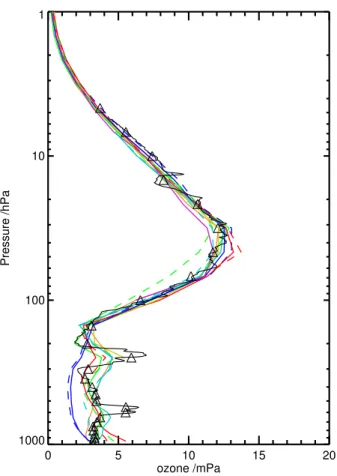
Figure 6 gives an example of the intercomparison, showing both the full-resolution

sonde profile and the layer-averages used to calculate statistics, alongside a number

of different analyses. Most of these capture a small bulge in ozone between 200 and

10

300 hPa, but do not capture the full strength of what is likely a laminar intrusion of stratospheric air.

3.3 HALOE

HALOE (Russell et al.,1993) uses solar occultation to derive atmospheric constituent

profiles. HALOE is used here as independent data for validation. Figure 7 shows

15

the coverage available. The nature of the solar occultation technique makes the data sparse in time and space, with about 15 observations per day at each of two latitudes. The horizontal resolution is 495 km along the orbital track and the vertical resolution is about 2.5 km.

We use an updated version 19 product, screened for cloud using the algorithm of 20

Hervig and McHugh(1999), and available from the HALOE website (http://haloedata.

larc.nasa.gov/). We found that, compared to the previously available version 19, the one with cloud screening substantially improved the quality of results in this intercom-parison around the tropical tropopause. Aside from the cloud screening, version 19 ozone retrievals are nearly identical to those of v18, and above the 120 hPa level they 25

agree with ozonesonde data to within 10% (Bhatt et al.,1999). Below this level, profiles

can be seriously affected by the presence of aerosols and cirrus clouds.

(20)

ver-ACPD

6, 4495–4577, 2006

A. J. Geer et al.

Title Page

Tables Figures

◭ ◮

Back Close

Full Screen / Esc

EGU

tical variation is smooth due to the much broader vertical resolution of the instrument. Hence, to compare to the analyses on common pressure levels, HALOE is simply in-terpolated between the nearest two of the 271 levels. Longitudes and latitudes vary with height in HALOE profiles but for this comparison, those at 10 hPa are taken to be representative of all levels.

5

3.4 TOMS

The Total Ozone Mapping Spectrometer (TOMS) measures backscattered ultraviolet radiances with high horizontal resolution (38 km by 38 km) and daily near-global cover-age. There are small gaps between orbital coverage bands near the equator. During the intercomparison period, due to the lack of sunlight at very high latitudes, there is 10

no data in July, August and September in the southern high latitudes; the same for October and November in the north. TOMS is not assimilated in any of the analyses evaluated here.

We use version 8 of the level 3 total column ozone product, which is a daily compos-ite of binned observations. Version 8 has partial corrections for calibration problems 15

in the post-2000 TOMS data from the Earth Probe satellite, and improved retrievals under extreme conditions (high observation angles, in the Antarctic, aerosol loading) compared to v7 (McPeters, personal communication, 2004). A full validation of TOMS v8 has not yet been published, but v7 uncertainties were estimated as about 2% for the random errors, 3% for the absolute errors and somewhat more at high latitudes due to 20

the higher zenith angle (McPeters et al.,1998).

4 Method

(21)

ACPD

6, 4495–4577, 2006

A. J. Geer et al.

Title Page

Tables Figures

◭ ◮

Back Close

Full Screen / Esc

EGU

so minimising colocation error when comparing with independent data. Based on the results of sensitivity tests (Sect.4.1), the choice of a 3.75◦ _{longitude by 2.5}◦ _latitude

grid, 37 fixed pressure levels, and twice daily analyses (00Z and 12Z) appears to be a reasonable compromise. Pressure levels are 6 per decade between 0.1 hPa and 100 hPa (as used on the Upper Atmosphere Research Satellite (UARS) project). Be-5

low this, there are levels at 150, 200 hPa, and so on every 50 hPa down to 1000 hPa. All comparisons against independent data, except those against TOMS, were made using analyses on the common grid. In the case of TOMS, experiments showed that going from the 50 levels of the DARC analyses to the 37 common levels caused a bias in total column calculations of between 3 DU and 7 DU. Hence, ozone columns 10

were calculated from analyses at their original vertical resolution. All vertical interpola-tions were done linearly in ln(P) (whereP is pressure) and all horizontal interpolation, bilinearly in longitude and latitude.

Statistics were built up from the difference between analyses and observations. In

this paper, statistics were binned in the regions referred to here as the southern and 15

northern high latitudes (90◦S to 60◦S and 60◦N to 90◦N, respectively), the southern and northern midlatitudes (60◦S to 30◦S and 30◦N to 60◦N respectively) and the trop-ics (30◦S to 30◦N). Statistics were binned monthly; also for the entire period 18 August 2003 to 30 November 2003 (before 18 August 2003, the DARC analyses were not adequately spun up).

20

Ozone amounts vary by many orders of magnitude through the atmosphere. Units of partial pressure emphasise the UTLS; units of mixing ratio emphasise the mid and up-per stratosphere. In order to give approximately equal weight through the atmosphere, statistics were normalised with respect to climatology, and displayed as a percentage.

As an example, for a particular bin (e.g. July in the tropics at 100 hPa), where i runs

25

(22)

ACPD

6, 4495–4577, 2006

A. J. Geer et al.

Title Page

Tables Figures

◭ ◮

Back Close

Full Screen / Esc

EGU

as

d =100×

1

n P

i(Ai −Ii)

c , (1)

wherecis the mean of the Logan/Fortuin/Kelder climatology at this level, for this month, and for this region (e.g. the tropics, 30◦S to 30◦N). This climatology does not go above 0.3 hPa, so at the top levels (0.21, 0.15 and 0.1 hPa) we use mean ozone from the 5

BASCOE v3q33 run instead. This particular approach to normalisation was chosen to reduce the influence of very small ozone amounts on the percentage statistics. If

a formulation is chosen that includes Ii in the denominator, d can show very large

percentage values at the tropical tropopause and in the ozone hole.

4.1 Sensitivity tests

10

We investigated the effect of the horizontal and temporal grid resolution on the

statis-tics of (Ai−Ii), by varying the time and space resolution of the ECMWF and DARC

analyses in comparisons to independent data. As previously described, the intercom-parison only considers analyses at 00Z and 12Z; hence independent data colocations are found within a time window of 12 h. We found that changing the spatial or temporal 15

resolution of the common grid had very little effect on the mean differences between

analysis and sonde. However, the standard deviations were affected in some regions

and Fig.8shows results for four selected time windows: 6, 12, 24 and 48 h. We first

consider the tropical stratosphere (Fig.8a), where changing the temporal and

horizon-tal resolution makes very little difference, and the horizontal and temporal variability of 20

ozone appears to be fairly small. The main regions where the temporal and spatial

resolution are important are the polar stratosphere (e.g. Fig. 8b) and the midlatitude

UTLS (e.g. Fig.8c). Here, time windows longer than 12 h appear to increase standard

deviations quite considerably. Increased spatial resolution is unimportant in the polar

regions, but does have a small e_ffect in the UTLS. Degrading spatial resolution further

25

(23)

ACPD

6, 4495–4577, 2006

A. J. Geer et al.

Title Page

Tables Figures

◭ ◮

Back Close

Full Screen / Esc

EGU

results are not shown. For the intercomparison, the 12 h time window and 3.75◦_{by 2.5}◦

grid appear a reasonable compromise.

In the mesosphere, there is a strong diurnal cycle in ozone (Sect.5.5). Figure9

ex-amines the e_ffect of this on the statistics of (BASCOE – HALOE) ozone for the tropical

region. Results at other latitudes are similar. Only the BASCOE analyses simulate a 5

diurnal cycle. In a special run of the assimilation system, profiles were generated at HALOE observation locations at the nearest model timestep, giving a maximum time mismatch of 15 min. Statistics generated using a 12 h time window are substantially different above 0.5 hPa, indicating the effect of the diurnal cycle. Hence in this work we do not show MIPAS or HALOE statistics above the 0.5 hPa level.

10

5 Results

This section first gives an overview of the results of the intercomparison, by examining statistics for the period 18 August 2003 to 30 November 2003. We first look at mean

differences compared to ozonesonde, HALOE and MIPAS (Sect. 5.1), then the

stan-dard deviations of these differences (Sect.5.2). We examine MIPAS calibration using

15

the analyses as a transfer standard (Sect. 5.3) and compare the analyses to TOMS

(Sect.5.4). Through most of the stratosphere, the analyses compare well to

indepen-dent data, but there are problems in the stratospheric polar vortex, at the stratopause and in the mesosphere, in the troposphere, in the extratropical UTLS, and at the

tropi-cal tropopause. A number of these regions are examined in more detail in Sects.5.5,

20

5.6and5.7.

5.1 Biases

Figures10,11and12show respectively the biases against HALOE, sonde and MIPAS,

(24)

ACPD

6, 4495–4577, 2006

A. J. Geer et al.

Title Page

Tables Figures

◭ ◮

Back Close

Full Screen / Esc

EGU

level if the number of colocations with data available is 50% (25% for MIPAS) of the total number of profiles. For example, less than half of sonde ascents reach the 10 hPa level

in the northern hemisphere (NH) high latitudes in Fig.11, so to avoid unrepresentative

results, this level is not plotted. Comparisons are not done above 0.5 hPa, because of the diurnal cycle in ozone.

5

For most of the stratosphere and mesosphere above 50 hPa, biases between the

analyses and HALOE, sonde and MIPAS are between−10% and 10%. The ECMWF,

DARC, and KNMI TEMIS analyses have larger biases in the upper stratosphere and mesosphere. DARC analyses have a positive bias which rises to 40% at 0.5 hPa. The bias is uniform at all latitudes and, by examination of the monthly statistics (not shown), 10

uniform in time. KNMI TEMIS analyses have a uniform negative bias, growing to−40%

at 0.5 hPa. Section5.5shows that the KNMI TEMIS and DARC biases result from the

linear chemistry schemes used in the models. The ECMWF bias is smaller, and has not been attributed, but again the linear chemistry scheme is the most likely explanation.

In the lower stratosphere (LS, 100 hPa to 50 hPa), analyses are biased typically 10% 15

high compared to sonde and HALOE, but reaching 50% at 100 hPa in the tropics.

Biases are typically smaller against MIPAS, reflecting a small (∼10%) positive bias

between MIPAS and the independent data at these levels (Sect.5.3). There are big

variations between different analyses in the lower stratosphere in the SH high latitudes

and near the tropical tropopause. These variations are examined in Sects.5.6and5.7,

20

respectively.

At SH high latitudes, KNMI TEMIS analyses stand out with a positive bias of 10 to 15% between 10 hPa and 30 hPa against MIPAS, HALOE and sonde. Above and below

this level, the bias becomes negative. There is a∼60% negative bias against sonde at

200 hPa. The KNMI TEMIS analyses are based only on total column observations; the 25

vertical profile is model-determined. To get a better vertical profile would require either model improvements or the assimilation of profile data (e.g.,Struthers et al.,2002).

The Juckes analyses are essentially unbiased when compared to MIPAS

(25)

ACPD

6, 4495–4577, 2006

A. J. Geer et al.

Title Page

Tables Figures

◭ ◮

Back Close

Full Screen / Esc

EGU

to MIPAS on pressure levels in Fig.12. These are likely explained by biases (e.g.,

De-thof,2004) between the MIPAS temperatures used to assimilate the data on isentropic

levels, and the ECMWF temperatures used here in the vertical transformation to pres-sure levels. This bias results in a small vertical uncertainty in the prespres-sure assignment of both the Juckes and MIMOSA ozone profiles.

5

In the troposphere (below 100 hPa), some analyses show quite substantial biases

when compared to sonde (Fig. 11). BASCOE analyses have a negative bias of

typ-ically 50% at all latitudes. DARC analyses have a large positive bias in the SH near the ground, associated with the Cariolle v1.0 scheme. MOCAGE-PALM Cariolle v2.1 analyses have a positive bias, particularly in the tropics, and this is known to be a 10

problem with v2.1 of the Cariolle scheme. There are no ozone profile observations

below∼400 hPa in any of the analyses, though the ECMWF system assimilates total

columns from GOME and partial columns from SBUV. None of the models represent detailed tropospheric chemistry. However, the MOCAGE-PALM Reprobus run does include upper-tropospheric chemistry. These analyses are quite successful in minimis-15

ing bias against ozonesonde, as are the ECMWF analyses, excluding the lowermost tropical troposphere. KNMI TEMIS analyses are also relatively successful; they simply impose a relaxation to tropospheric climatology. In general, the most likely explanation for the tropospheric biases is limitations in the ozone chemistry schemes used in the other models, on top of a lack of observational data.

20

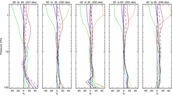
Next we examine biases in the KNMI SCIAMACHY profile analyses. SCIAMACHY profiles were only available in quantity for assimilation for October and November dur-ing the intercomparison period. November analysis biases against sonde are shown

in Fig.13; October biases are similar, as are the results against HALOE and MIPAS.

In the NH in the lower stratosphere (200 to 10 hPa), the SCIAMACHY profile analyses 25

have up to 20% negative bias compared to sonde and are notably di_fferent from the

(26)

ACPD

6, 4495–4577, 2006

A. J. Geer et al.

Title Page

Tables Figures

◭ ◮

Back Close

Full Screen / Esc

EGU

SH high latitudes. SCIAMACHY profiles do not go below∼12 km, thus this is due to

the relaxation of the photochemical scheme towardsFortuin and Kelder(1998)

clima-tology. Against HALOE and MIPAS (figures not shown) biases are no more than+20%

in the upper stratosphere and mesosphere, which is comparable in magnitude to many of the other analyses (Figs.10and12).

5

5.2 Standard deviations

Figures14,15and16 show the standard deviations of differences between analyses

and HALOE, sonde and MIPAS ozone respectively, normalised against climatology

(see Sect.4). As a reference point, these figures also show the standard deviations of

the differences between observations and the Logan/Fortuin/Kelder climatology. Again,

10

statistics are only plotted at a particular level if the number of colocations is 50% (25% in the case of MIPAS) of the total number of profiles available.

Analyses demonstrate smaller standard deviations than climatology throughout the high latitude stratosphere, and in the midlatitude lower stratosphere and upper tropo-sphere (10 hPa to 300 hPa). In other regions, particularly the tropical stratotropo-sphere, 15

analyses do little better, or even worse, than climatology. These are regions of rela-tively low synoptic variability, and in the upper stratosphere, ozone is close to photo-chemical equilibrium. By contrast, at high latitudes in the stratosphere, ozone transport is important and there is strong synoptic variability. Looking at the monthly statistics (not shown), the analyses demonstrate the largest improvements over climatology at 20

high latitudes in September, October and November. In the SH, there is strong syn-optic variability due to the onset of the top-down breakup of the polar vortex (e.g.,

Lahoz et al.,2006). In the NH, synoptic variability is likely associated with increasing surf-zone activity around the developing vortex during these months. The midlatitude UTLS is also a region of high variability in ozone. Ozone has strong gradients across 25

the tropopause; in data assimilation systems these gradients are expected to provide dynamical information, particularly on the horizontal position of the polar front (e.g.,

(27)

ACPD

6, 4495–4577, 2006

A. J. Geer et al.

Title Page

Tables Figures

◭ ◮

Back Close

Full Screen / Esc

EGU

In the mid and upper stratosphere (above 50 hPa), standard deviations are typi-cally less than 10% against HALOE and (to 10 hPa only) sonde data. However, there are some exceptions. DARC analyses are worse above the 1 hPa level; this is likely due to problems with the linear photochemistry scheme. ECMWF analyses have rela-tively high standard deviations (15%) versus HALOE in the SH high latitudes, between 5

10 hPa and 1 hPa. This may be associated with the ozone photochemistry scheme, or it could be due to known problems in ECMWF upper stratospheric temperatures at

high latitudes (Randel et al., 2004). Standard deviations of the DARC and ECMWF

analyses against MIPAS are also larger compared to the other analyses in the upper stratosphere, supporting the conclusions drawn from HALOE, and suggesting that the 10

model is dominating over the MIPAS observations. KNMI TEMIS analyses also show relatively large standard deviations against MIPAS in the high latitude upper strato-sphere, compared to the other analyses, but this might be expected since these are the only analyses in which MIPAS is not assimilated.

In the lower stratosphere (between 50 hPa and 100 hPa), standard deviations against 15

sonde, HALOE and MIPAS become larger than in the upper stratosphere. In the

mid-latitude comparisons (30◦_{S to 60}◦_{S and 30}◦_{N to 60}◦_{N) analyses show standard}

de-viations against MIPAS, HALOE and sonde, of ∼20% at 100 hPa. At high latitudes

and in the tropics, standard deviations are larger. At 100 hPa in the tropics, there is disagreement between the data types. The standard deviations of (analysis – sonde) 20

are∼30%, compared to∼85% for MIPAS and∼70% for HALOE. This suggests a large

degradation in the quality of the satellite retrievals at these levels, which is likely due to

the effects of undetected cloud, as well as the sharp vertical gradients in temperature

and ozone. The degradation in quality of HALOE retrievals at 100 hPa is already

well-known (e.g.,Bhatt et al., 1999). Section 5.3investigates MIPAS data quality further.

25

At the tropical tropopause and in the SH high latitude lower stratosphere, compared

to sonde, there are notable differences between the analyses themselves. These are

examined in more detail in Sects.5.6and5.7.

(28)

ACPD

6, 4495–4577, 2006

A. J. Geer et al.

Title Page

Tables Figures

◭ ◮

Back Close

Full Screen / Esc

EGU

and 80% (Fig.15). None of the analyses does better than climatology at levels below

400 hPa; above this level the analyses do demonstrate improvements over climatology. DARC and ECMWF analyses show large standard deviations in the SH. The explana-tion for the high standard deviaexplana-tions in the troposphere is likely the same as for the large biases: no ozone profile information is assimilated below 400 hPa and the ozone 5

photochemistry schemes do not simulate tropospheric chemistry well. KNMI TEMIS analyses do relatively well in the troposphere with a simple relaxation to climatology.

5.3 MIPAS validation

Previous sections have indicated di_fferences in ozone amounts between MIPAS,

ozonesonde and HALOE. Using the analyses as a transfer standard, we can examine 10

the bias between MIPAS and independent data. This has the advantage, compared to colocating pairs of observations, that all available observations are included in the sample. Note that in all comparisons here, MIPAS data are treated as point retrievals and the analyses are interpolated to the MIPAS retrieval points linearly in ln(P) in the vertical. It is well known that comparison in terms of radiances, or the use of averaging 15

kernels (Rodgers,2000;Migliorini et al.,2004), produces a better representation of the information content of the retrievals; these methods are increasingly used in calibration and validation activities. But here, no assimilation system uses MIPAS radiances or an averaging kernel representation (both the subject of much ongoing research), so it is the bias in MIPAS retrievals, treated as a point values, that is important.

20

The bias between MIPAS and sonde can be estimated from the statistics shown in

Figs.10,11and12as, for example, (MIPAS – sonde)=(MIPAS – analysis) – (sonde –

analysis). Figure17summarises the biases calculated using BASCOE v3q33 analyses

as the transfer standard. These are chosen for their small standard deviations against

independent data through the stratosphere (Figs. 14 and 15), though Fig. 17 would

25

in general be similar no matter which analyses are chosen (figures not shown). The

sampling patterns of sonde and HALOE vary with time (Figs.5and7) and the biases

(29)

ACPD

6, 4495–4577, 2006

A. J. Geer et al.

Title Page

Tables Figures

◭ ◮

Back Close

Full Screen / Esc

EGU

are broadly typical of the period.

In the upper stratosphere (above ∼30 hPa), MIPAS measures approximately 5%

more ozone than HALOE. In the lower stratosphere (100 to 30 hPa), MIPAS has a

high bias of typically 10% compared to sonde and HALOE. ExceptingMigliorini et al.

(2004), this lower stratospheric bias is a consistent feature of other studies that have 5

considered the calibration of MIPAS for a variety of periods and data versions (Dethof,

2003a,b,2004;Fischer and Oelhaf,2004;Wargan et al.,2005;Geer et al.,2006). At 100 hPa in the tropics and midlatitudes, MIPAS appears unbiased against HALOE and sonde. However, if statistics are calculated by interpolating from MIPAS retrieval

points to the intercomparison fixed pressure levels, biases at 100 hPa are +20% in

10

the midlatitudes and₊50% in the tropics (figures not shown). The fixed pressure levels

are more closely spaced than the MIPAS retrievals. Because, particularly at the tropical tropopause, there is a sharp transition between very low tropospheric ozone values and much higher stratospheric ones, interpolation tends to increase the ozone amounts. Also noting that previous studies do not provide consistent conclusions on the biases at 15

100 hPa in the tropics and midlatitudes, the results should here be treated with caution. Elsewhere in the stratosphere, however, the biases are essentially insensitive to the vertical interpolation strategy. Standard deviations also appear mostly insensitive to interpolation strategy at 100 hPa and above.

At 200 hPa, the high bias against HALOE is likely a problem with HALOE observa-20

tions. Biases between MIPAS and sonde below 100 hPa are relatively small, except in the SH at 300 hPa, though again a sensitivity to the interpolation strategy mean these results should be treated with caution.

Finally, we examine the fact that standard deviations between MIPAS and analyses

are in some cases much larger than between sonde and analyses. Section5.2noted

25

that, at the tropical tropopause, MIPAS standard deviations are∼85%, compared to

∼30% for sonde. The MIPAS and sonde sampling patterns are quite different (Figs.4

and 5). Ozonesondes are concentrated just south of the equator for the SHADOZ