SPATIAL CORRELATION OF SOYBEAN PRODUCTIVITY, ENHANCED VEGETATION INDEX (EVI) AND AGROMETEOROLOGICAL VARIABLES

Engineering

ISSN: 1809-4430 (on-line)

_________________________

1 _{Universidade Federal da Grande Dourados - UFGD/Dourados, Brasil.} 3 _{Universidade Estadual do Oeste do Paraná - UNIOESTE/Cascavel, Brasil.} 4 _{Universidade Estadual do Oeste do Paraná - UNIOESTE/Cascavel, Brasil.}

SPATIAL CORRELATION OF SOYBEAN PRODUCTIVITY, ENHANCED VEGETATION INDEX (EVI) AND AGROMETEOROLOGICAL VARIABLES

Doi:http://dx.doi.org/10.1590/1809-4430-Eng.Agric.v37n3p541-555/2017

DENISE M. GRZEGOZEWSKI1_{, MIGUEL A. URIBE-OPAZO}2*_,

JERRY A. JOHANN3_{, LUCIANA P. C. GUEDES}4

2*_{Corresponding author. Universidade Estadual do Oeste do Paraná - UNIOESTE/ Cascavel - PR, Brasil.}

E-mail: miguel.opazo@unioeste.br

ABSTRACT: The survey information from growing regions, the interaction with the vegetation index and climatic variables is of great importance in the search for soybean productivity increase. Paraná is the second largest soybean producer in Brazil and presents great spatial variability, both in periods of the crop cycle as in soil and climate. The objective of this study was to analyze the spatial correlation of soybean productivity, the enhanced vegetation index (EVI) and agrometeorological variables (water balance, global radiation and average temperature) in the state of Paraná, on a decendial scale, using the Moran global autocorrelation index between the 2010/2011 and 2012/2013 crop years. Similarity was found in the average productivities in 2010/2011 and 2012/2013. In 2011/2012 the state average was 2.38 t ha-1 _{lower in 10.19%}

compared to the national average, caused by the water deficit in flowering and grain filling phases. As a consequence, spatial autocorrelation indicated a higher similarity in productivity among municipalities with a Moran index of 0.735. The use of vegetation indices and agrometeorological variables allowed the identification of different sowing periods between regions and great climatic variability, influencing the soybean productivity.

KEYWORDS:culture cycle, spatial statistics of areas, climatic variability.

INTRODUCTION

Soybean cultivation is of great importance in the world agriculture, according to FAOSTAT (2015) the production in 2010, 2011, 2012, 2013 and 2014 were respectively 265; 261; 241; 277 and 306 million tons worldwide. In Brazil, soybean is the most important of all commodities produced and plays a key role in the country’s economy, besides being the world’s second largest producer of soybeans. However, according to CONAB (2014) in the 2011/2012 crop year, drought in the Brazilian producing regions has reduced production. With favorable climatic conditions, in the crop year of 2012/2013, 29.43% of all soybeans produced in the world were produced in Brazil, and the state of Paraná being the second largest producer of this commodity in the country.

To estimate the production it is necessary to know the cultivated areas with the species of interest and its productivity in different regions (ASSAD et al., 2007). The crops productivity can also be estimated from agrometeorological models (FONTANA et al., 2001). Among the agrometeorological factors, water availability, photoperiod and temperature are the factors that most affect soybean productivity (FARIAS et al., 2007). Thus, the effects of water deficit depend on its intensity, duration, time of occurrence and interaction with other determining components of the final productivity (FONTANA et al., 2001).

uniform emergence. On the other hand, temperatures above 40ºC are harmful to the crop, with adverse effects on the growth rate, flowering, and decrease the pod retention capacity. Thus, the growth, development and productivity of an agricultural crop are affected by climatic variability (VIRGENS FILHO et al., 2013).

The interaction among the plant, the environment and the management defines the productivity, thus, obtaining high productivity is only possible when environmental conditions are favorable throughout the crop cycle (GILIOLI et al., 1995). Another factor that influences the crop productivity is the different cultivars used, which vary from region to region.

The spatial statistics of areas (SSA) is one of the ways to evaluate this variability, since it allows comprehending and understanding the spatial distribution of the data. Studies in this area are becoming more common (DALPOSSO et al., 2013, PRUDENTE et al., 2014) due to the availability of geographic information systems (GIS), that allows us to present a map of the spatial patterns of the desired variables (CÂMARA et al., 2002), using global indicators that measure the correlation of the variable in time or space (ARAÚJO et al., 2013), such as the Moran Global Index (BAILEY & GATRELL, 1995).

Thus, the aim of this study was to analyze the spatial correlation of soybean productivity, the enhanced vegetation index (EVI) and the meteorological variables represented by water balance (Cw), global radiation (Gr) and average temperature (Te) in decendial scale, for the 2010/2011 to 2012/2013 crop years in the state of Paraná.

MATERIAL AND METHODS Study area

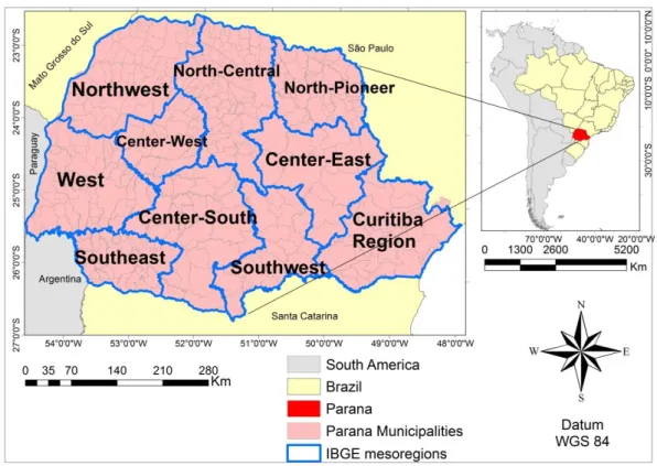
The study area comprises the state of Paraná, with 399 municipalities, divided according to IBGE ten mesoregions (Figure 1) (Northwest, West, Southwest, Center-West, Center-South, Center-East, Southeast, Curitiba Region, North-Central and North-Pioneer).

Data acquisition

Average soybean yield data

Data from the average yield (t ha-1_{) of Parana municipalities for the crop years studied were}

obtained from the Paraná Secretariat of Agriculture and Supply (SEAB). For the 2010/2011, 2011/2012 and 2012/2013 crop years, respectively, 37, 38 and 31 municipalities did not contain information on average yield.The national productivity averages were obtained from the Brazilian Institute of Geography and Statistics (IBGE).

Vegetation index data derived from the MODIS sensor

Many studies related to agricultural crop monitoring have used images of the Improved Vegetation Index (EVI) (HUETE et al., 1997; JOHANN et al., 2012, SOUZA et al., 2015) since it has the advantage of being less susceptible to saturation and more sensitive to the structure variation, canopy architecture and plant physiognomy (HUETE et al., 2002). In this study, EVI images of the MOD13Q1.5 product of the Moderate Resolution Imaging Spectroradiometer (MODIS) sensor were obtained on board the Terra satellite of the "Tile" h13v11, which has a spatial resolution of 250 m and a temporal resolution of 16 days of the database products of the Brazilian Agricultural Research Corporation (ESQUERDO et al., 2010). The images period for each crop year was from August 13 to April 23 of the following year, which is considered the period in which soybean is grown in the state (JOHANN et al., 2012; JOHANN et al., 2016).

The mapping of soybean cultivated areas in Paraná for the 2010/2011 and 2011/2012 crop years was obtained from SOUZA et al. (2015) and for the crop year 2012/2013 from GRZEGOZEWSKI et al. (2016). From these mappings, the average EVI values of the soybean-mapped pixels of the entire time series of images (JOHANN et al., 2013) were extracted for each municipality, by means of automated routines developed in interactive data language (IDL) (ESQUERDO et al., 2011).

Rescheduling of EVI vegetation index data for decendial scale

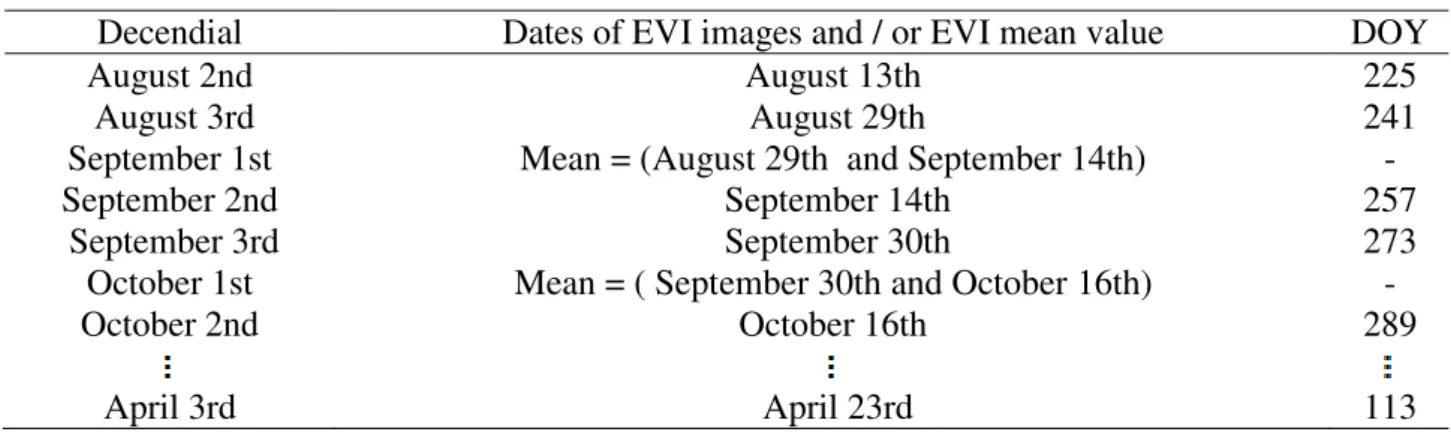
As the original EVI vegetation index data (16 day temporal resolution) had a different scale from the agrometeorological (decendial) data, the EVI time series data from each municipality were rescheduled to the decendial scale (Table 1), following the procedure Proposed by JOHANN (2012).

TABLE 1. Rescheduling EVI data method (16 days) to the decendial scale.

Decendial Dates of EVI images and / or EVI mean value DOY

August 2nd August 13th 225

August 3rd August 29th 241

September 1st Mean = (August 29th and September 14th) -

September 2nd September 14th 257

September 3rd September 30th 273

October 1st Mean = ( September 30th and October 16th) -

October 2nd October 16th 289

April 3rd April 23rd 113

Source: Adapted from JOHANN (2012). Note: DOY: Day of the year.

Agrometeorological data

{MJ m-2 _day-1_{} and mean air temperature (Te) {ºC} from September to April of each crop year. It}

was necessary to adapt the agrometeorological data of the 303 virtual stations (Figure 2-a) to the spatial scale of 399 municipalities. For each decendial and for each municipality a value was determined, which corresponds to the mean values of the virtual stations of each agrometeorological variable contained in and around the polygon, as exemplified in Figure 2-b for a municipality.

FIGURE 2. Representation of the regular network of the 303 virtual stations of the European Center for Medium-Range Weather Forecasts (ECMWF) (a) and virtual stations used to obtain the municipal average of each agrometeorological variable (b).

Spatial autocorrelation analysis

The spatial proximity matrix W is used to represent how the neighborhood influences each

observation, expressing the spatial structure of the data. According to ANSELIN et al. (2007), is a square matrix with elements, where each element represents a measure of spatial proximity between populations (counties) and , which can be calculated from criteria. The contiguity criterion (tower, queen, and bishop) specifies that , if shares a common side with , otherwise ; for (ANSELIN et al., 2007). In the present study, the Queen contiguity criterion was adopted, which characterizes a municipality as a neighbor of a municipality if has a border or common node with , that is, considering the whole neighborhood.

To estimate how much the observed value of an attribute in a region is dependent on the values of this same variable, in the neighboring locations, the Moran Index (I_MG)(MORAN, 1950) was determined (Equation 1), which ranges from -1 (perfect negative autocorrelation), 0 (absence of autocorrelation) and +1 (perfect positive autocorrelation).

  

 

ij i j

i=1 j=1

MG n n n 2

ij i

i=1 j=1 i=1

w x - x x - x n

I =

w x - x



where,

n: sample size;

i

x and x : value of the considered attribute in area i and j (i, j = 1, ..., n); j

x: mean value of the attribute in the study region, ij

w : elements of the normalized matrix of spatial proximity.

RESULTS AND DISCUSSIONS

Analysis of soybean municipal average yield and variables under study

According to FERREIRA et al. (2007), the long-term variations in crop yields are caused by factors related to new management techniques, new varieties and quality improvement and efficiency of agricultural inputs.On the other hand, short-term changes in productivity, that is, from one crop year to the next, are mainly due to climate change.

As the second largest soybean producer in the country, the state of Paraná had in 2014/2015 crop year, a cultivated area of approximately 5.24 million hectares, production of approximately 17.23 million tons and average productivity of 3.29 T ha-1 _{(IBGE, 2015).Analyzing the 2010/2011}

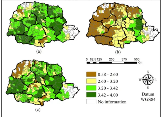
crop year (Figure 3-a), some municipalities located in the Northwest and Southeast regions obtained yields lower than 2.60 t ha-1_{. In 2011/2012 (Figure 3-b), it was found that the average municipal}

productivity of soybean was lower than 3.20 t ha-1 _{in practically the whole state, except part of the}

Eastern Center region.It is noteworthy that, in large producing regions such as the West, Southwest and Center West of Paraná, the highest productivity was 2.60 t ha-1_.

FIGURE 3. Spatial maps of soybean yield (t ha-1_{) for the 2010/2011 (a), 2011/2012 (b) and}

2012/2013 (c) crop years. Source: SEAB (2015).

In the crop year 2012/2013 (Figure 3-c), productivity in regions with higher yields approached historical averages. However, in the Northwest region, the municipal average productivity was found in the lowest class from 0.58 to 2.60 t ha-1_{, as in the previous crop year.}

that the Northwest region is characterized as an area unfavorable to soybean cultivation, with a high risk of drought occurrence during the most critical phenological phases (flowering and Fruiting) of the development of the crop. This explains the results obtained for the North-west mesoregion of the last two crop years, indicating a lower productive potential in relation to other mesoregions of the State.

Among the harvested years, soybean mean yields different to 5% significance were observed (Table 2). However, the crop year of 2011/2012 had a decrease in average productivity of approximately 1.00 t ha-1 _{in relation to the other crop years studied, due to climatic adversities,}

according to FERREIRA et al. (2007). In the comparison between state and national average yields, there was also a statistically significant difference at 5% probability, with state averages at 7.14% and 9.52% higher for the 2010/2011 and 2012/2013, respectively, and 7.54% lower than the national average for 2011/2012.

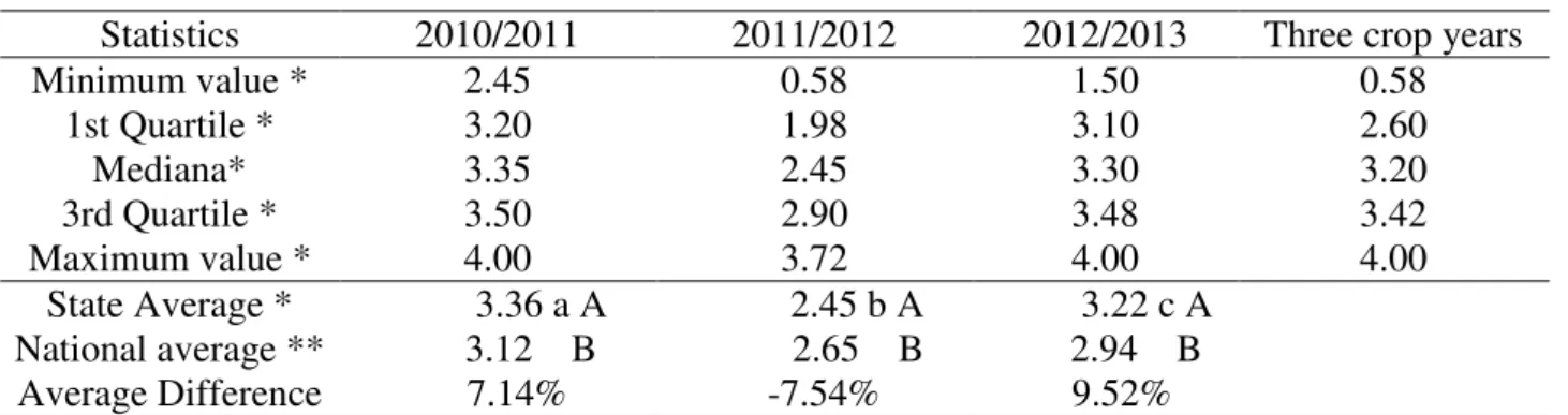
TABLE 2. Descriptive statistics for soybean yield (t ha-1_{) in three crop years studied.}

Statistics 2010/2011 2011/2012 2012/2013 Three crop years

Minimum value * 2.45 0.58 1.50 0.58

1st Quartile * 3.20 1.98 3.10 2.60

Mediana* 3.35 2.45 3.30 3.20

3rd Quartile * 3.50 2.90 3.48 3.42

Maximum value * 4.00 3.72 4.00 4.00

State Average * 3.36 a A 2.45 b A 3.22 c A National average ** 3.12 B 2.65 B 2.94 B Average Difference 7.14% -7.54% 9.52%

*Official Data (SEAB, 2015) **(IBGE, 2015). Different capital letters indicate significant mean differences between State and National productivity; lowercase letters indicates significant average differences between crop years. (t-Student Test, 5% significance).

FIGURE 4. Average state decendial by crop year of enhanced vegetation index (EVI) (a) and agrometeorological variables; water balance [Cw] (b), global radiation [Gr] (c) and average temperature [Te] (d).

FIGURE 5. Spatial maps of the variables of enhanced vegetation index (EVI) and water balance (Cw) for each studied decendial and crop years 2010/2011, 2011/2012 and 2012/2013.

In general, for the 2010/2011 crop year, there was a water deficit (municipalities in blue and yellow in Figure 5), since the values of the water balance (Cw) were negative, indicating that the evapotranspiration was higher than the precipitation, for most of the municipalities, until the 2nd decendial of November (exception for the 3rd decendial of September). After this period, water availability did not affect crop development and productivity, as shown in Figure 3-a and Table 2.

As for the crop year 2011/2012, early sowings were identified in relation to other crop years since the 2nd decendial of November (Figure 5); municipalities in the Western region of Paraná were already with high EVI values (0.496 to 0.881). However, unlike 2010/2011, the positive Cw (Figure 5), which indicates more precipitation than evapotranspiration, only occurred until the 2nd decendial of November.

After this period, until the first decendial of January (Figure 5), Cw values were negative (water deficiency) for most of the municipalities of the state, a period that coincides with the reproductive development phase until practically the crop harvest what justifies the low average state productivity (Figure 3-b) of 2.45 t ha-1 _{(Table 2).}

BETTOLLI et al. (2003) pointed out that, in Argentina, soybean yield is a function of precipitation in the months of November and December and the maximum temperature in January. Thus, good climatic conditions at this time, that is, water availability that is determined mainly by the association between positive water balance and ideal temperatures are a good indicator of high productivity.

The soil temperature range suitable for sowing varies from 20°C to 30°C (FARIAS et al., 2007), and should be avoided if it is below 20°C as it compromise germination and plant emergence. Thus, for 2010/2011 (Figure 6), sowing could be carried out from the 1st decendial of September. However, in this period in the state of Paraná, there is a measure that prohibits the planting or maintenance of live soybean plants between May 15 and September 15 (ADAPAR, 2015). This measure is called a sanitaryemptiness, which aims to avoid or delay the appearance of the fungus that causes Asian rust, a disease that attacks the crop, causes economic losses and losses in productivity.

For 2011/2012, the high radiation (Gr) caused evapotranspiration increase, that is, the water evaporated from the soil and transpired by the plants in the growth phase was not uniformly. According to FARIAS et al. (2011), the Gr is the triggering factor of photosynthesis, in which atmospheric CO2, with the participation of water is transformed into carbohydrates. These

carbohydrates are used for the growth and maintenance of the crop; however, at this plant phase, the droughts occurred, damaging the final productivity in practically the whole state.

Spatial correlation analysis

By analyzing the spatial data, the hypothesis was confirmed that the productivity spatial distribution is not random, so, there is a positive correlation in the data (Table 3).This means that in terms of global scale, the Moran index (I_MG) indicates that in Paraná there are municipalities with high or low productivity surrounded by municipalities with the same situation.

TABLE 3. Moran index (I_MG) for soybean yield in the three-year harvest.

Index 2010/2011 2011/2012 2012/2013

MG

I _{0.552* 0.735* 0.627*}

*Significant indexes at 0.05 level of probability.

FIGURE 6. Spatial maps of solar radiation (Gr) and mean air temperature (Te) for each studied decendials and crop years 2010/2011, 2011/2012 and 2012/2013.

JOHANN et al. (2016).As the soybean crop was sown (Figures 4 and 5) in October and November (FIGUEIREDO et al., 2016), the spatial autocorrelation among municipalities has decreased (Figure 7-a), indicating that the vegetation indices in this period are heterogeneous in the state, that is, they varied among regions.

FIGURE 7. Moran spatial autocorrelation of the variables:enhanced vegetation index EVI (a), water balance [Cw] (b), global radiation [Gr] (c) and average temperature [Te] (d) for each decendial in the state of Paraná.

In the 2011/2012 crop year, the EVI spatial autocorrelation index was higher (Figure 7-a), which indicates greater similarity of EVI throughout the State. This occurred, according to CARVALHO et al. (2008), because the vegetation indexes are proportional to the photosynthetic activity, presenting higher values when this activity is higher and there is greener biomass. Even if there were early harvests in some municipalities, the rapid implantation of other crops (corn second harvest), in soybean sequence, it kept the Moran indices high, and therefore similar in the State. In the three decendials of December and 1st _{of January, there was some anomaly in relation to other}

crop years studied. The Moran indexes found during this period decreased, showing that the vegetation indexes were affected and, therefore, considered heterogeneous among the municipalities in this development phase of the soybean crop. Under this focus, it is appropriate to say that productivity is affected by the agrometeorological variables in this period and in several regions.

From January onwards the EVI indices for the three years harvests were similar, indicating spatial homogeneity among Paraná’s municipalities. For the 2010/2011 crop year, in January, smaller values of the spatial autocorrelation index were found when compared to 2011/2012 and 2012/2013.This is justified by the spatial variability in the sowing in the state municipalities. Thus, areas with early sowing had their harvest anticipated, which led to the occurrence of dissimilar autocorrelation.

high and similar, according to the number of decendials. This demonstrates that if the Cw was positive (i.e. with water available for the plant) in a municipality, its neighbors also had this characteristic, as well as in the state. In contrast, in another period within the cycle, municipalities with negative Cw (i.e., water deficit for the plant) had as neighboring municipalities also with a negative water balance.

CONFALONE & NAVARRO-DUJMOVICH (1999) reported that the solar radiation (Gr) remains relatively constant in the different phenological stages of the soybean crop, growing in optimal conditions when it has non-limiting water conditions. The global autocorrelation indices (IMG) for this variable (Figure 7-c) were high, indicating homogeneity between regions. However, for the crop year 2011/2012 in which there was a water deficit (Figure 5) over a long period of the soybean cycle, the efficiency of the use of solar radiation was reduced.This efficiency, according to CASAROLI et al. (2007), can lead to light saturation when the culture is subjected to high intensities of absorbed solar radiation.

The spatial autocorrelation for the average temperature (Figure 7-d) during the soybean cycle was high in the state, indicating similarity among the municipalities, so, low spatial variability. According to MELLO et al. (2008), increases in air temperature may cause increase in surface evaporation, causing changes in the Cw and thus affecting the crop.

Also, the lack of precipitation can cause high temperatures for several days, especially in the hottest months (December and January), that according to SILVA et al. (2009) can affect the growth and development of plants, reducing photosynthesis, respiration and dry matter production.

CONCLUSIONS

The study showed differences between the harvested years studied for soybean yield:

 These differences were influenced by climatic factors during critical phases of the crop cycle. Among the climatic factors, the lack of precipitation caused by the negative water balance, together with the high global radiation, evapotranspiration and temperatures in the sowing and crop development phases affected the final productivity.

 By the EVI vegetation index, it was identified soybean sowing variability in the regions of the state, however, its intra-annual variation depends on adequate water conditions for the producer to start planting.

 By the analysis of spatial autocorrelation, greater similarities were identified in the crop year 2011/2012 with lower yields that is, due to the drought observed by the water balance, the spatial autocorrelation index was similar in Paraná’s municipalities due to the lower variability of the soybean yields.

ACKNOWLEDGEMENTS

We would like to thanks to CAPES, CNPq and Araucaria Foundation for financial support.

REFERENCES

ADAPAR. Agência de Defesa Agropecuária do Paraná. Portaria ADAPAR nº 193,de 6 de outubro de 2015. Estabelece o período de semeadura para a cultura da soja entre 16 de setembro a 31 de dezembro de cada ano agrícola no Estado do Paraná. Curitiba. 2015.

ARAÚJO, E. C.; URIBE-OPAZO, M. A.; JOHANN, J. A. Análise de agrupamento da variabilidade espacial da produtividade da soja e variáveis agrometeorológicas na região Oeste do Paraná.

Engenharia Agrícola, Jaboticabal, v. 34, n. 4, p.782-795, jul./ago. 2013. DOI: 10.1590/S0100-69162013000400018

ASSAD, E. D.; MARIN, F. R.; EVANGELISTA, S. R.; PILAU, F. G.; FARIAS, J. R. B.; PINTO, H. S.; ZULLO JÚNIOR, J. Sistema de previsão da safra de soja. Pesquisa Agropecuária

Brasileira, Brasília, DF, v. 42, n. 5, p. 615-625, maio 2007.

BAILEY, T. C.; GATRELL, A. C. Interactive spatial data analysis. Essex: Longman Scientific, 1995. 432 p.

BETTOLLI, M. L.; PENALBA, O. C.; VARGAS, W. M. Relación entre el rendimiento de la soja y las variables climáticas en la Pampa Húmeda Argentina. In: CONGRESSO BRASILEIRO DE AGROMETEOROLOGIA, 13., 2003, Santa Maria: Anais... Disponível em:

<http://www.conicet.gov.ar/new_scp/detalle.php?keywords=&id=23281&congresos=yes&detalles= yes&congr_id=80112>.

CARVALHO, F. M. V.; FERREIRA, L. G.; LOBO, F. C.; DINIZ-FILHO, J. A. F.; BINI, L. M. Padrões de autocorrelação espacial de índices de vegetação Modis no bioma cerrado. Revista Árvore, Viçosa, MG, v. 32, n. 2, p. 279-290, mar./abr. 2008. DOI:

10.1590/S0100-67622008000200011

CÂMARA, G.; CARVALHO, M. S.; CRUZ, O. G.; CORREA, V. Análise Espacial de Área. In FUCKS, S. D.; CARVALHO, M. S.; CÂMARA, G.; MONTEIRO, A. M. V. Análise espacial de dados geográficos. São José dos Campos: Instituto Nacional de Pesquisas Espaciais, Divisão de Processamento de Imagens, 2002. Disponível em:

<http://www.dpi.inpe.br/gilberto/livro/analise/cap1-introducao.pdf>.

CASAROLI, D.; FAGAN E. B.; SIMON, J.; MEDEIROS, S. P.; MANFRON, P. A.; NETO, D. D.; LIER, Q. J. V.; MÜLLER, L.; MARTIN, T. N. Radiação solar e aspectos fisiológicos na cultura de soja - uma revisão. Revista da Faculdade de Zootecnia, Veterinária e Agronomia, Uruguaiana, v. 14. n. 2, p. 102-120, 2007. Disponível em:

<http://revistaseletronicas.pucrs.br/ojs/index.php/fzva/article/view/2502/1961>.

CONAB - Companhia Nacional de Abastecimento. Acompanhamento da safra brasileira de grãos, v. 1 - Safra 2013/14, n. 12 - Décimo Segundo Levantamento. Brasília, 2014. p. 1-127. Disponível em:

<http://www.conab.gov.br/OlalaCMS/uploads/arquivos/14_09_10_14_35_09_boletim_graos_setem bro_2014.pdf>. Acesso em: 24 set. 2015.

CONFALONE, A.; NAVARRO-DUJMOVICH, M. Influência do “déficit” hídrico sobre a

eficiência da radiação solar em soja. Revista Brasileira de Agrociência, Pelotas, v. 5, n. 3, p. 195-198, 1999. DOI: 10.18539/cast.v5i3.292

DALPOSSO, G. H.; URIBE-OPAZO, M. A.; MERCANTE, E.; LAMPARELLI, R. A. C. Spatial autocorrelation of NDVI and GVI indices derived from LANDSAT/TM images for soybean crops in the western of the state of Paraná in 2004/2005 crop season. Engenharia Agrícola, Jaboticabal, v.33, n.3, p. 525-537, maio/jun. 2013. DOI: 10.1590/S0100-69162013000300009

DIAS, F. T. C.; PITOMBEIRA, J. B.; TEÓFILO, E. M.; BARROS, F. S. Adaptabilidade e estabilidade fenotípica para o caráter rendimento de grãos em cultivares de soja para o Estado do Ceará. Revista Ciência Agronômica, Fortaleza, v. 40, n. 1, p. 129-134, jan./mar. 2009. Disponível em: <http://www.redalyc.org/pdf/1953/195318130019.pdf>.

ESQUERDO, J. C. D. M.; ANTUNES, J. F. G.; ANDRADE, J. C. de. Desenvolvimento do banco de produtos MODIS na Base Estadual Brasileira. Campinas: Embrapa Informática

Agropecuária, 2010. 7p. (Comunicado Técnico, 100).

ESQUERDO, J. C. D. M.; ZULLO JUNIOR, J.; ANTUNES, J. F. G. Use of NDVI/AVHRR time series profiles for soybean crop monitoring in Brazil. International Journal of Remote Sensing, London, v. 32, n. 13, p. 3711–3727, jun. 2011. DOI: 10.1080/01431161003764112.

FAOSTAT - FOOD AND AGRICULTURE ORGANIZATION OF THE UNITED NATIONS.

ProdSTAT – Crops. 2015. Disponível em: <http://faostat3.fao.org/download/Q/QC/E 2015>. FARIAS, J. R. B; NEPOMUCENO, A. L.; NEUMAIER, N. Ecofisiologia da soja. Londrina: EMBRAPA-CNPSo, 2007. 9p. (Circular Técnica, 48).

FARIAS, J. R. B. Limitações climáticas à obtenção de rendimentos máximos de soja. In

CONGRESO DE LA SOJA DEL MERCOSUR, 5.; FORO DE LA SOJA ASIA, 1., 2011, Rosário.

Anais… Un grano: un universo. Rosário: Asociación de la Cadena de la Soja Argentina, 2011. 4 p.

Disponível em: <http://www.alice.cnptia.embrapa.br/handle/doc/906919>.

FERREIRA, W. P. M.; COSTA, L. C.; SOUZA, C. de F. Teste de um modelo agrometeorológico para estudo da influência da variabilidade climática na cultura da soja. Revista Ceres, Viçosa, MG, v. 54, n. 312, p. 207-214, 2007. Disponível em:

<http://www.redalyc.org/articulo.oa?id=305226740002>.

FIGUEIREDO, G. K. D. A.; BRUNSELL, N. A.; HIGA, B. H.; ROCHA, J. V.; LAMPARELLI, R. A. C. Using correlation maps to assess soybean yield from EVI data in Paraná state, Brazil. Scientia Agricola, Piracicaba, v. 73, p. 462-470, 2016. DOI: 10.1590/0103-9016-2015-0215

FONTANA, D. C.; BERLATO, M. A.; LAUSCHNER, M. H.; MELLO, R. W. Modelo de estimativa de rendimento de soja no Estado do Rio Grande do Sul. Pesquisa Agropecuária Brasileira, Brasília, DF, v. 36, n. 3, p. 399-403, mar. 2001. DOI:

10.1590/S0100-204X2001000300001

GILIOLI, J. L.; TERASAWA, F.; WILLEMANN, W.; ARTIAGA, O. P.; MOURA, E. A. V.; PEREIRA, W. V. Soja: Série 100. Cristalina: FT Sementes, 1995. 18p. (Boletim Técnico 3). GRZEGOZEWSKI, D. M.; JOHANN, J. A.; URIBE-OPAZO, M. A.; MERCANTE, E.

COUTINHO, A. C. Mapping soya bean and corn crops in the State of Paraná, Brazil, using EVI images from the MODIS sensor. International Journal of Remote Sensing, London, v. 37, p. 1257–1275, fev. 2016. DOI: 10.1080/01431161.2016.1148285

HUETE, A., LIU, H. G., BATCHILY, K., LEEUWEN, W. J. D. V. “A comparison of Vegetation Indices over a Global Set of TM Images for the EOS-MODIS”. Remote Sensing of Environment, New York, v. 59, p. 440-451. 1997. DOI: 10.1016/S0034-4257(96)00112-5

HUETE, A.D.L.; DIDAN, K.; MIURA, T.; RODRIGUEZ, E.P.; GAO, X.; FERREIRA, L.G. Overview of the radiometric and biophysical performance of the MODIS vegetation indices.

Remote Sensing of Environment, New York, v. 83, p. 195-213, 2002. DOI: 10.1016/S0034-4257(02)00096-2

IBGE - INSTITUTO BRASILEIRO DE GEOGRAFIA E ESTATÍSTICA. Banco de dados agregados - Sistema IBGE de Recuperação Automática – SIDRA. 2015. Disponível em: <http://www.sidra.ibge.gov.br>. Acesso em: 24 jun. 2015.

JOHANN, J. A. Calibração de dados agrometeorológicos e estimativa de área e produtividade de culturas agrícolas de verão no Estado do Paraná. 2012.225f. Tese (Doutorado em

JOHANN, J. A.; ROCHA, J. V.; DUFT, D. G.; LAMPARELLI, R. A. C. “Estimativa de áreas com culturas de verão no Paraná, por meio de imagens multitemporais EVI/MODIS”. Pesquisa

Agropecuária Brasileira, Brasília, DF, v. 47, n. 9, p. 1295-1306, set. 2012. DOI:10.1590/S0100-204X2012000900015

JOHANN, J. A.; ROCHA, J. V.; OLIVEIRA, S. R. DE M.; R., LUIZ H. A.; LAMPARELLI, R. A. C. Data mining techniques for identification of spectrally homogeneous areas using NDVI temporal profiles of soybean crop. Engenharia Agrícola, Jaboticabal,v. 33, n. 3, p. 511-524, maio/jun. 2013. DOI: 10.1590/S0100-69162013000300008

JOHANN, J. A.; BECKER, W. R.; URIBE-OPAZO, M. A.; MERCANTE, E. Uso de imagens do sensor orbital Modis na estimação de datas do ciclo de desenvolvimento da cultura da soja para o estado do Paraná – Brasil. Engenharia Agrícola, Jaboticabal, v. 36, n. 1, p. 126-142, jan./fev. 2016. DOI: 10.1590/1809-4430

MELLO, E. L.; OLIVEIRA, F. A.; PRUSKI, F. F.; FIGUEIREDO, J. C. Efeito das mudanças climáticas na disponibilidade hídrica da bacia hidrográfica do Rio Paracatu. Engenharia Agrícola, Jaboticabal,v. 28, n. 4, p. 635-644, out./dez. 2008. DOI: 10.1590/S0100-69162008000400003 MORAN, P.A.P. Notes on continuous stochastic phenomena, Biometrika, Cambridge, v. 37, n. 1-2, p. 17-23, jun. 1950. DOI: 10.2307/2332142

PRUDENTE, V. H. R.; SOUZA, C. H. W. DE; MERCANTE, E.; JOHANN, J. A.;

URIBE-OPAZO, M. A.; Spatial statistics applied to soybean production data from Paraná state for 2003-04 to 2009-10 crop-years. Engenharia Agrícola, Jaboticabal, v. 34, n. 4, p. 755-769, jul./ago. 2014. DOI: 10.1590/S0100-69162014000400015

SAKAMOTO, T.; YOKOZAWA, M.; TORITANI, H.; SHIBAYAMA, M.; ISHITSUKA, N.; OHNO, H. A crop phenology detection method using time-series MODIS data. Remote Sensing of Environment, New York, v. 9, n. 6, p. 366-374. 2005. DOI: 10.1016/j.rse.2005.03.008.

SAKAMOTO, T. B. D.; WARDLOW, A. A.; GITELSON, S. B.; VERMA, A.; SUYKER, E.; ARKEBAUER, J. J. “A Two-Step Filtering Approach for Detecting Maize and Soya bean

Phenology with Time-Series MODIS Data.” Remote Sensing of Environment, New York, n. 10, v.114, p. 2146–2159, 2010. DOI: 10.1016/j.rse.2010.04.019

SEAB - SECRETARIA DA AGRICULTURA E DO ABASTECIMENTO DO PARANÁ /

DEPARTAMENTO DE ECONOMIA RURAL. Produção agrícola Paranaense. 2015. Disponível em: <http://www.agricultura.pr.gov.br/modules/conteudo/conteudo.php?conteudo=137>. Acesso em: 20 nov. 2015.

SILVA, R. A. B.; SOUZA, A. L. F.; CAMPOS, P. M.; BILICH, M. R.; ROCHA, J. V. Estimativa de área plantada de soja utilizando imagens MODIS, no Estado de Goiás.In: SIMPÓSIO

BRASILEIRO DE SENSORIAMENTO REMOTO, 14., 2009, Nadal. Anais... p. 483-489. Disponível em: <http://marte.dpi.inpe.br/col/dpi.inpe.br/>. Acesso em: 31 set. 2015.

SOUZA, C. H. W. de; MERCANTE, E.; JOHANN, J. A.; LAMPARELLI, R. A. C.; URIBE-OPAZO, M. A. Mapping and discrimination of soya bean and corn crops using spectro-temporal profiles of vegetation indices. International Journal of Remote Sensing, London, v. 36, p. 1809-1824, abr. 2015. DOI: 10.1080/01431161.2015.1026956