Analysis of the response of polymer composites under off-axis loading with skewed tabs

(1)

Analysis of the response of polymer composites under off‐axis loading with skewed tabs. J.Cros. FEUP

CONTENTS ... 1 1 INTRODUCTION ... 2 2 REVIEW ... 6 2.1 New tab design: Selection of materials ... 6 2.2 New tab design: A new oblique‐shaped end tab ... 7 3 EXPERIMENTAL PROGRAM ... 13 3.1 Specimen design ... 13 3.2 Review: DIC technique ... 15 3.3 Manufacture process ... 18 3.4 Photomechanical set‐up and measurement parameters ... 21 4 ANALISIS METHODS ... 24 4.1 Experimental data ... 24 4.2 Failure criteria ... 29 4.3 Numerical analysis ... 34 5 CONCLUSIONS... 38 6 REFERENCES ... 40

(2)

1 INTRODUCTION

In today’s competitive aerospace and military industry, the weight and strength are of critical importance. This has led to the widespread use of various different types of long fiber composite materials. In order to take full advantage of the weight saving offered by composites, it is necessary to have an accurate understanding of the individual laminate properties. Both the material elastic constants and the ultimate strengths are of importance.

Off‐axis specimens have been used to produce shear deformation and stress in fiber composites by simple axial loads. The key advantage in using off‐axis specimens lies in the fact that a combined state of stress with respect to the material principal directions can be produced simply with a uniaxial load.

For this reason, the tensile test on unidirectional off‐axis fiber composites is a fundamental test which has been successfully employed for a number of years by researchers in the field of composite materials to characterize the response of these advanced materials. Not only has the test been used to obtain in‐plane lamina properties such as E11, E22, v12 and the related strengths,

but also to verify the material‐symmetry assumptions of the particular system. The off‐axis configuration has also been employed by numerous researchers in determining the in‐plane or intra laminar shear modulus G12.

There are a number of different test methods currently used to obtain the properties of composites materials. Those are alternatives to performing direct torsion test on thin composites tubes. Torsion test are more difficult and expensive to fabricate. Rail shear test have a number of disadvantages: it is very hard to produce a pure shear over the test section, and the test fixture introduces large stress concentrations. Coupon tests of the any off‐axis specimen also have problems due to the fact that a state of combined stress rather than pure shear exists in such a laminate and that it is very difficult to detect the first ply failure and to avoid lamination effect on the ply strength.

The next and last test method proposed uses off‐axis specimens of unidirectional composite. This method seems ideal; easy specimen fabrication, very simple data reduction and requiring no special equipment. In order to extract the material constants from an off‐axis test, it is assumed that a uniform state of both stress and strain exists throughout the surface test section.

In the other hand, it has been known for some time that the off‐axis configuration can introduce errors in the measured values of the laminate elastic material parameters due to the extension‐

(3)

behaviour. If the ends of the sample are rigidly gripped and prevented from rotation, as dictated by a material’s natural response, during applied pure axial displacement at the grips, a highly inhomogeneous state of deformation will be induced in the specimen.

a) Unconstrained b) Constrained

Figure 1: Influence of end constraints in the testing of anisotropic bodies [Ref.3]

Figure 1a) shows the deformed state of an off‐axis specimen subject to uniaxial tension. If the ends are constrained to remain horizontal through the use rigid clamps, both shearing and bending moments are introduced as shown in figure 1b). These induced forces and moments produce a non‐uniform strain field which is not suitable for measuring the basic material properties.

Using the standard transformation relations, the shear stress ז12 in the local coordinate system at the midpoint of the specimen is: ) sin (cos cos sin 2 2 12 σ θ θ τ θ θ τ =− xx + xy − Equation (1)

Where זxy is the shear stress in the laminate coordinate (global system) induced by the end

constrains in the presence of shear‐coupling.

However, in practice, it has been customary to ignore the shear stress contribution זxy induced by

(4)

θ θ σ

τ *₁₂ = − 'xx.sin .cos Equation (2)

As will be subsequently illustrated, the shear stress in the material principal coordinates, ז12 given

by the correct transformation, equation (1), is smaller in magnitude for the considered composite system than the apparent shear stress ז*12 given by equation (2) for a wide range of important

test configurations. The difference between the correct and incorrect stress transformations in determining the shear response in the material principal coordinate system respectively is graphically illustrated bellow. a) End constraint effect included b) End constraint effect excluded Figure 2: Resolved shear stress in the material coordinate system with and without the influence of end constrains [Ref.3]

Dividing the relation between the correct shear stress ז12, and the apparent shear stress ז*12 by

the shear strain γ12, and defining the pretend shear modulus, G12 = ז*12 / γ12, the following ratio,

indicative of the error introduced in calculating the shear modulus, G12. So, this helps to bring the

forth fact that the error is caused by the use of the incorrect transformation equation in calculating the resolved shear stress ז12.

(5)

In a similar manner as that used to derive the expression for the apparent shear modulus G*12, the

expression for the apparent laminate Young’s modulus E*xx can be obtained. Here, this expression

is derived on the basis of the average laminate stress σxx as is commonly done in practice.

Substituting the relation between זxy and σxx and the relation between σxx and σ’xx.

When comparing the error introduced in the determination of the shear modulus G12 and the

Young’s modulus Exx with end‐constraint effect ignored, it is instructive to note that the general

form of the equations for the respective apparent quantities is the same. As conclusions from the above comparison is that the end‐constraint phenomenon has a much more pronounced adverse effect on determination of G12 than on Exx, also the adverse effect is most pronounced for the low

off axis angles (0>30 deg) and increases with decreasing specimen aspect ratio. For highly anisotropic composites, very long and slender 10‐deg off‐axis specimens are required to reduce the error in G12 caused by the end‐constraint effect to an acceptable level. The 45 deg off‐axis

coupon is an excellent specimen for accurate determination of the intralaminar shear modulus G12.

To minimize and solve these and other problems, Richards & Airhart and Pipes & Cole [Ref.1] suggested using very long tapered fiberglass tabs. These tabs redistribute the load gradually and may reduce the high stress concentrations at the clamps. This method of using long tapered tabs still results in stress concentrations, not as severe as in the case of short no tapered tabs. Fabrication becomes very time‐consuming and expensive when using such tapered tabs. Chang [Ref.2] tested with a pinned‐end test frame and compared the results with those from rail‐shear test and from standard, clamped, in 10° off‐axis tests. The pinned specimen resulted in higher ultimate shear strength and shear strain than either of the other type of test. Sun and Berreht [Ref.3] proposed end‐tabs made of fiberglass knit and silicon rubber matrix. This was verified to produce a uniform state of strain. The disadvantage of this tab is that it cannot sustain applied load at elevated temperature, and that it takes time to fabricate.

The purpose of the present study is to investigate and performed a detailed experimental investigation of the mechanical response of composites under multi‐axial loading using off‐axis tensile test specimens in different fiber orientations. The tensile strength was measured using oblique tab, and the experimental results were compared with the tensile strength predicted based on the Puck failure criterion [Ref.9]. This failure criterion is discussed for predicting the tensile strength at a high strain rate. This investigation requires a previous definition of the proper load introduction systems, including the development the of analysis models for skewed tabs.

(6)

2 REVIEW

2.1 New tab design: Selection of materials

One of the main objectives of this study is to find the tab’s material properties and geometry necessary to allow shear deformation under these tabs. The tab must be made in a different material and orientation than those of the specimen. The high stress concentrations and non‐ uniformities throughout the stress field in off‐axis tests are caused by the restriction of shear deformation. In order to solve the problem the load must be applied in a way which allows shear deformation. A tab between the specimen and grip which allows shear deformation can solve the problem. A number of different compliant materials which offer very poor shear rigidity came to mind as possible solutions. Unidirectional composites, soft adhesive layers, and rubber tabs were all tried with poor results [Ref.1] Test performed with various soft tab materials brought to light another problem. The tab must be very stiff in the thickness direction or the grips tend to crush the unidirectional coupons. An orthogonally woven fiberglass cloth exhibits all the desired characteristics. Cloths have high transverse and longitudinal stiffness with very little shear rigidity. With this in mind two different types of fiberglass cloths were moulded into a soft matrix of silicon rubber. The first type of fiberglass tried is a standard grade cloth, the second material type is knit, that consist of a layer of unidirectional fiberglass laid transversely over another layer of unidirectional fiberglass and knit together using polyester thread.

In the follow table, the results of material properties are shown [Ref .1]. Each coupon was placed in an MTS 810 material testing system. The specimen was then gripped in MTS 647 hydraulic wedge grips under 273 kg pressure. The tabs were placed on the test coupons and secured in place with a thin bans of tape. Several glues were tries with no success. All the glues tried failed to form a proper bond with the smooth surface of the silicon rubber. Care must be taken to properly align the tabs with the specimen to achieve the best results. The fiberglass knit tabs must be placed on the specimen with transverse fiber direction next to the specimen. This placement is required to minimize crushing after securing in the hydraulic grips.

(7)

Table 1: Properties of tabbing materials [Ref .1]

The tab composed of silicon rubber and fiberglass was not capable of achieving extremely high loads. During the test it was found that the tab could transmit loads up to 680 Kg. Loads higher than this resulted in the fiberglass knit failing and, thus, the specimen slipped out of the grips. The conclusion is that new end tab fabricated of fiberglass knit and a complaint silicon rubber matrix allowed shear deformation to occur in off‐axis composite specimens clamped by hydraulic grips. This capability enabled the off‐axis specimen to achieve a uniform strain field and, thus, is suitable for characterization of mechanical properties of unidirectional composites. Further, the new tab design makes it possible to use short specimens for testing without inducing the undesirable stress concentration effect produced by the conventional rigid tab. Although shear strength must be determined by using a failure criterion when off‐axis specimens are used, the procedure is not sensitive to other strength values (longitudinal and transverse strengths) used when small off‐axis angles are selected. Moreover, if a failure theory is to be used in general failure analyses, this procedure will allow the shear strength to absorb whatever inherent inaccuracy the failure criterion has and yield and accurate overall strength prediction.

2.2 New tab design: A new obliqueshaped end tab

Test specimens of fiber off axis composites under uniaxial loading exhibit different stress/strain behaviour depending on the fiber orientation relative to the loading direction. In this study will analyze off‐axis coupon with several fiber orientation to determinate composite properties such as strains, strengths, etc.

As previous as mentioned, in order to extract the behaviour results from an off‐axis test, it is required that a uniform state of stress exist throughout the test section. The problem with the off‐ axis test is that, the application of constant end displacement induces shearing forces and bending moments in the specimen, resulting in stress concentration and non‐uniform deformation. This must be solved with a new tab design: an oblique‐shaped end‐tab. Comparison of the

Material E1 (MPa) ν12 G12 (MPa) E1/G12

Fiberglass knit 4136 0.20 4.89 845:1

(8)

deformation in the specimen [Ref.2]. So, this phenomenon indicates that the strain distribution is not uniform in the case of conventional tabs. It causes a premature failure at the tabbed area due to stress concentration.

A simple formulation for the oblique angle was derived for any fiber orientation, C.T Sun [Ref.2]. Consider an off‐axis composite specimen under the uniaxial stress σxx=σ0. The state of

deformation is given by the strain as:

‐ εxx= S11 σ0 ‐ εyy= S12 σ0

‐ γxy= S16 σ0 Equation (1)

Where, Sij of the matrix are the compliance coefficients with respect to the xy coordinate system,

from the compliance matrix in plane stress, figure 3. Figure 3: Matrix compliance in off‐axis lamina plane stress analysis It is evident that shear deformation occurs from the application of a normal load, except when the xy coordinate system coincides with the material principal axes.

(9)

Analysis of the response of polymer composites under off‐axis loading with skewed tabs. J.Cros. FEUP Figure 4: Off‐axis specimens with (a) rectangular tabs (b) oblique tabs The integration of strain/displacement relations yields the displacement components: u = εXXx + f(y) v = εyyy + g(x) Equation (2) Where, f(y) and g(x) are arbitrary functions of the respective arguments. For the constant strain field given by Equation (1), f(y) and g(x) assume the form: f(y) = C1y + C3 g(x) = C2x + C4 Equation (3) Where, Ci are arbitrary constants. Therefore, the displacements in Equation (2) are: u = S11.σ0x + C1y + C3 v = S12. σ0y + C2x + C4 Equation (4) Removing the rigid body translations, we set C3 = C4 = 0. If we assume that the vertical edge of the specimen remains vertical after deformation, then:

(10)

0 2 = = ∂ ∂ C x v Equation (5) The remaining constants C1 can be determinate by the known shear strain as follows.

( )

'

( )

1 ' x f y C g y u x v ₌ ₊ ₌ ∂ ∂ + ∂ ∂ = γ Equation (6)

From equations (1) and (6), C1 is found to be S16σ0. Thus, the displacement field is obtained as:

y S v y S x S u 0 12 0 16 0 11 . . . σ σ σ = + = Equation (7), (8) From Equation (7), it is noted that the vertical component of displacement (u) can be maintained uniformly along a straight line satisfying the equation:

(

11 16

)

0 0 S x S yσ u = + Equation (9) Considering a straight line (x) with an angle Φ in (figure 4) relative to the x‐axis given by: 11 16 cot S S − = φ or 16 11 tan S S − = φ Equation (10) Using equation (10) and the material properties, it can found any oblique angle of end tabs (Φ), as from any specimen’s fiber orientation (θ) desired. Matlab routine is written to define the results through the graphical, as the next figure shows.

(11)

Analysis After th axis spe compos that the Further result i dynami for the from ea [Ref.10 s of the respo Figure 5: G he analytica ecimen, the site propert e oblique ta r, it is found s encourag c tensile str 60° and 7 ach other; t ]. onse of polym Graphite of o al and nume e oblique a ties. Both t ab is far sup d that the f ging becaus rength of of 5° off‐axis this is beca mer composi oblique angl erical study, ngle was o the finite e perior to the failure posi se it implie

ff‐axis spec in the conv use in thes ites under off e for oblique , from a sim obtained as lement ana e conventio tion is mai es that the imen. It is w ventional a se cases the ff‐axis loadin e end‐tabs in mple analysi a function alysis and e nal rectang nly in the g e oblique ta worthwhile nd oblique e extension g with skewe n function of s of the def of the off‐ experimenta gular tab.

gauge sectio ab is applic to note, tha tabs are n ‐shear coup ed tabs. fiber orienta formation f ‐axis angle al results h on of the s cable for e at the strain not significa pling effect J.Cros. FEU ation field in the o and from t elped confi specimen. T evaluating t n distributio antly differe is quite sm UP off‐ the irm This the ons ent mall

(12)

Figure 6: Geometry of the tabs used in this study for each fiber orientation respectively

(13)

3 EXPERIMENTAL PROGRAM

This chapter presents all the information on the experimental programme: The geometry including the new oblique end tab design, previously explained in the review, as well as the manufacture process. Testing in one side of the specimen has been done by (DIC), digital image correlation, to get accurate measurements of the displacements and of the strains during deformation. On the other side, it was planned to use the rosette‐strain gauges, in order to verify if appears the stress concentrations and to compared the output results in both methods. Unfortunately, was not possible to glue them.

3.1 Specimen design

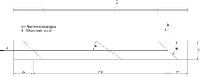
The specimens are fabricated by IM7‐8552 carbon epoxy with different off axis fiber orientation. Three specimens were manufactured for each fiber orientation. The thickness of the specimen is 1.5 mm.

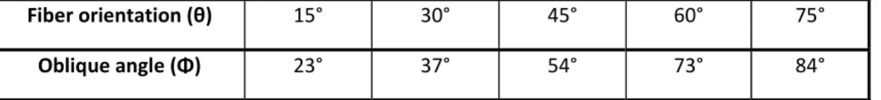
The end tabs were cut from aluminium sheets and then were bonded on the specimens using “Thermoset Plastics 103 epoxy adhesive”. The employed oblique angle tabs are show, in the follow table, as a function of fiber orientation angle from the graphical (Figure 5). The thickness of the tabs is the same as that of the specimens (1.5 mm). Fiber orientation (θ) 15° 30° 45° 60° 75° Oblique angle (Φ) 23° 37° 54° 73° 84° Table 2: Oblique angle desired for each specimen orientation fiber required

Figure 7 presents the proposed specimen geometry with the dimensions. The oblique angle changes in function of the fiber orientation. The proposed angles are showed in table 2. Moreover are showed the specimens ready for testing in figure 8.

(14)

Figure 7: Geometry specimens with oblique tabs (in mm) Figure 8: The specimens tested in this study, one for each orientation

(15)

3.2 Review: DIC technique

Digital image correlation (DIC) is a whole‐field and non‐contact deformation measuring method. It provides deformation information of a specimen by processing two digital images, which are captured before and after the deformation. As compared to the special requirements of the traditional optical measurements, such as photo elasticity or holography, DIC is an easy and cheap method because it takes advantage of the natural speckle pattern on the specimen surface and only digital images taken by charge coupled device (CCD) camera are processed. Afterward, the displacements are measured by DIC‐software and compared to the imposed ones. Using this method the matrices of the displacements and strains on the studied plane are obtained.

Figure 9: Working principle of the DIC system [Ref.6]

Compared with the interferometric optical techniques used in this study (in‐plane deformation measurement, the DIC method has both advantages and disadvantages. For instance, it offers the following special and attractive advantages. • Simple experimental setup and specimen preparation: only one fixed CCD camera is needed to record the digital images of the test specimen surface before and after deformation. • Low requirements in measurement environment, 2D DIC does not require a laser source. A white light source or natural light can be used for illumination during loading.

(16)

• Wide range of measurement sensitivity and resolution: Since the 2D DIC method deals with digital images, thus the digital images recorded by various high‐spatial‐resolution digital image acquisition devices can be directly processed by the DIC method. However, the 2D DIC method also suffers some disadvantages. • The test planar object surface must have a random gray intensity distribution • The measurements depend heavily on the quality of the imaging system Figure 10: Measuring principle: Stochastic pattern, photogrammetric principle and calibration plate [Ref.6]

Normally, the positions of the reference points and the nearby point after deformation are not located at the pixel points of the digital image, and there are no grey level values for these points. Hence, interpolation is necessary to recover their grey level values such that the intensity pattern of the subset can be obtained.

On using the discrete pixels of a digital image and their grey level values for intensity, these data are recorded as a two dimensional array. Under the assumption that there is a one‐to‐one correspondence on the intensity pattern of two images taken before and after during application of the load, one can deduce the deformation information from the intensity pattern. A subset is arbitrarily chosen from the image taken before a deformation increment and a reference point (x0, y0) as well as a close point (x, y) is selected from this subset as shown in figure 11, the position (x’, y’) of the nearby point after the deformation increment can be described as: , Equation (11) , Equation (12)

(17)

Where (u, v) are the displacements of the reference point, and (dx, dy) are the position differences of the reference point and the nearby point before deformation. The components of the first order displacement gradient are denoted as ∂v/∂x, and ∂v/∂y. Since only a two dimensional deformations is considered in the above equation, one needs two displacement components and four displacement gradient components to describe the position of a nearby point [Ref.6]. Figure 11: Schematic of subsets before and after deformation [Ref.6]

Correlation computations often require the estimation of the image gray levels for non integer pixel locations. In our study, a bilinear interpolation is used. This it works from the grey level value I(x,y) at a point located between four pixel points is obtained as: , Equation (13) Where ai are constants, which can be obtained from the grey level values of the four nearby pixel points. Under the supposition and limit described above, one can find a subset in the deformed image that is correspondent to the un‐deformed subset by considering the displacements gradients. To represent the correlation of these two subsets, a cross‐correlation coefficient or at least squares correlation coefficient is commonly used.

The measurements of DIC depend on a number of factors, including both the performance of hardware and correlation algorithm details. It is difficult or impossible to isolate one error source form the others, so the effects of these factors (speckle pattern, out‐of‐plane displacement, lens distortion, noise, subset size, sub‐pixel registration algorithm, shape function, interpolation) have been investigated to improve them, in previous specialized studies. Based to them, are extracted

(18)

• Experimental conditions:

• Increase the contrast of the speckle pattern

• Guarantee parallelism between the CCD target and the test planar specimen surface • Use a telecentric lens

• Use a high‐quality low noise CCD camera and keep stable and even illumination during loading • Algorithm details: • Use a larger subset when the shape function matches the underlying deformation field • Use the improved software method to optimize the correlation criterion • Use a high‐order shape function • Use a bicubic spline or biquintic B‐spline interpolation scheme With a history of more than 20 years, DIC has been improved by many researchers and developed into an effective and flexible optical technique for surface deformation measurement from the macroscopic to micro‐ or even nanoscale. Recall that 2D DIC can only be used for in‐plane deformation of a planar object. So, for deformation measurement of a macroscopic object such as structural components hence, is perfectly suited for testing the samples of this job [Ref.6].

3.3 Manufacture process

The composite material used is Hexcel IM7‐8552. This is a high performance tough epoxy matrix for use in primary aerospace structures. It exhibits good impact resistance and damage tolerance for a wide range of applications. It has features and benefits, as toughened epoxy matrix with excellent mechanical properties, elevated temperature performance, good translation of fibre properties, controlled matrix flow in processing, and available on various reinforcements [Ref.12]. The manufacturing process starts by cutting the pre‐peg. Then, staked each one with the help of glue film which includes, each plate has 12 plies (totally 36 plies for 3 plates), and the thickness of each ply is 0.125 mm. The plates are cured in a hot‐press, following the cycle shown bellow (Figure 12).

(19)

Analysis of the response of polymer composites under off‐axis loading with skewed tabs. J.Cros. FEUP Figure 12: Curing cycle for monolithic composites [Ref.12] Heat is applied at a rate of 1‐3ºC/min to 110ºC ± 5ºC with 2 bar pressure, then hold at the same temperature for 60 minutes ± 5 minutes, below heat ramping up again until to 180ºC ± 5ºC, and hold at the same temperature during 120 minutes ± 5 minutes. Then, cool at 2‐5ºC per minute until room temperature.

After curing the plates, they were cut to the final geometry with the help of diamond disk. The tabs were cut from the aluminum sheets in the workshop. With the specimens and tabs already cut, they are bonded using aThermoset Plastics 103 epoxy adhesive.

When the specimens and tabs were glued together, they are ready for being clamped by the hydraulic grip fitted on the testing machine. Static unidirectional tests were performed with stroke control using a hydraulic servo testing machine at room temperature (~18 ºC). Before the test, the specimen side surface used must have a random gray intensity distribution (the random speckle pattern), which deforms together with the specimen surface as a carrier of deformation information. When this texture does not naturally exist on the material, different techniques have been successfully used for creating such a pattern. In this work, the speckle pattern was artificially created applying a thin coating of white spray paint followed by a spread distribution of spots of black spray paint, as is showed in the right side (Figure 13). The test consisted in two parts. The digital image correlation technique was used on one side of two specimens in each orientation, previously described in the preceding paragraph.

(20)

Figure 13: The specimens before and after spraying the random speckle pattern In a specimen of each orientation, strain gauges 2 and 3 were mounted in the wing and the other one in the middle of the specimen surface. The next figure shows the locations of the strain gauges. Figure 14: Distribution of strain gauges on the specimen surface It is also required to set the rosette‐strain gauges, especially in the sharpest oblique tabs. Because is the DIC camera cannot focus the area close the tabs. These gauges provided the ε in from σ

(21)

in global coordinates, and then were processed for each orientation in laminate coordinates (material) from the matrix transformation.

After the DIC test, the yield and failure points of the strain‐stress curves were obtained. These values are applied together with the in LaRC curve of the theoretical failure criteria. Further, the specimens were analyzed by numerical methods to check to stress concentrations, and therefore to verify the effectiveness of the new design tabs. The results are shown and discussed in the next chapters. The strain gauges 2 and 3, close to the tabs, did not stick together after applying the glue to the specimen’s surface. The main reason was that there is not enough place to apply pressure after gluing the strain gauge. Therefore, was decided to use the results of C.T. Sun and OLSUP CHUNG [Ref. 2] because these authors used the same specimen geometry. 3.4 Photomechanical setup and measurement parameters

In this work, the ARAMIS‐ 2D DIC software by GOM® was used. The measurement system is equipped with an 8‐bit Baumer Optronic FWX20 camera (resolution of 1624x1236 pixels size of 4.4 μm and sensor format of 1/1.8'') coupled with a Nikon AF Micro‐Nikkor 60 mm f/2.8D lens. For mobility and adaptability, the support of the cameras was mounted on Foba ALFAE tripod, which was positioned facing the testing machine.

In the set‐up, the optical system was positioned with regard to the surface of the specimen, mounted into the testing machine. A laser pointed was used to guarantee a correct alignment. The working distance (defined between the specimen’s surface and the support of the cameras) was set about 0.5 mm; leading to a conversion factor of about 0.029 mm pixel‐1 (table 3). The lens was adjusted to be in focus with regard to the surface of interest, setting the lens aperture to f/2.8 in order to minimise the depth of field. The aperture of the lens was then closed to f/16 in order to improve the depth of field during the test. The shutter time was set to 8 ms, according to the cross‐head displacement rate during testing (2.5 mm min1) and the size of the camera unit cells (4.4 μm). The light source was finally adjusted in order to guarantee an even illumination of the specimen’s surface and to avoid over‐exposition (the saturation of pixels over the field of view).

(22)

Figure 15: Experimental setup

In the digital image correlation method, as described above, the displacement field is measured by analysing the geometrical deformation of the images of the surface of interest, recorded before and after loading. For this purpose, the initial (un‐deformed) image is mapped by square facets (correlations windows), within which an independent measurement of the displacement is calculated. Therefore, the facet size, on the plane of object, will characterise the displacement spatial resolution. The facet step (the distance between adjacent facets) can also be set either for controlling the total number of measuring points over the region of interest or for enhancing the spatial resolution by slightly overlapping adjacent facets. Typically, a great facet size will improve the precision of the measurements but also will degrade the spatial resolution. Thus, a compromise must be found according to the application to be handled. In this work, a facet size of 15x15 pixels was chosen, attending to the size of the region of interest, the optical system (magnification) and the quality of the granulate (average speckle size) obtained by the spray paint. The in‐plane displacements were then numerically differentiated in order to determine the strain field need for the material characterisation problem. In order to evaluate the displacement resolution of the method, a set of static images were taken without applying any load. By processing this sequence of images a noise signal is obtaining. The statistical processing of this signal can allow an overall evaluation of the resolution of the method.

(23)

Typical values for the displacement resolution were in the range of 10‐2. Table 4 shows the parameters of the test setup. Project parameter‐ Facet Conversion factor 0.029 mm/pixel Facet size 15 pixels Step size 15 pixels Project parameter‐ Strain computation size 5 macro‐pixel Validity code 55% Strain computation method Total Test speed 1 mm/min Camera rate 0,5 frame per second Image recording – Acquisition frequency 1 Hz Table 4: Parameters used in the ARAMIS‐GOM® software

(24)

4 ANALISIS METHODS

During this study, two different analysis methods were used: experimental test by DIC and numerical analysis doing the discretization of the samples by the finite element method (FEM). The goal of this chapter is to obtain the result for each method, and to compare the different results. In this manner, the validity of failure criteria used in this study is verified.

4.1 Experimental data

The results obtained from the experimental tests performed on off‐axis tension tests on unidirectional composites by the DIC method, explained in the preceding paragraph, are shown in the following figures. The stress time curves with the ratio of stresses, of each specimen separately (Figure 16) provides the information about failure points, are then compared between LaRC failure criteria (Figure 18) in the transverse‐shear stress envelope. The stress‐strain curve obtained for all fiber orientation angles is shown in Figure 17.

The figures are named using the initials OAT (off axis tension), and number of the angle orientation followed by the number of test, for example (OAT 15º‐1). The ratio for each orientation angle is: OAT | | | . |

(25)

Analysis of the response of polymer composites under off‐axis loading with skewed tabs. J.Cros. FEUP Ratio OAT 15 = 3,7320 Ratio OAT 30 = 1,7320 0 50 100 150 200 250 300 350 0 0,2 0,4 0,6 0,8 1 1,2 Str e ss (M Pa) Strain (%) 15º‐1 15º‐2 15º‐3 0 20 40 60 80 100 120 140 160 180 200 220 240 260 280 300 320 340 360 1 11 21 31 41 51 61 71 81 91 Stres s (M Pa) Time (s) 15º‐1 15º‐2 15º‐3 slope 0 20 40 60 80 100 120 140 160 180 0 0,2 0,4 0,6 0,8 1 1,2 1,4 Str e ss (M Pa) Strain (%) 30º‐1 30º‐2 30º‐3 0 15 30 45 60 75 90 105 120 135 150 165 180 195 210 225 240 1 11 21 31 41 51 61 71 81 91 Stres s (M Pa) 30º‐1 30º‐2 30º‐3 slope

(26)

Ratio OAT 45 = 1 Ratio OAT 60 = 0,5773 0 20 40 60 80 100 120 0 0,2 0,4 0,6 0,8 1 1,2 1,4 Stress (M P a) Strain (%) 45º‐1 45º‐2 45º‐3 0 10 20 30 40 50 60 70 80 90 100 110 120 130 140 1 11 21 31 41 51 61 71 σxx Str e ss (M Pa) Time (s) 45º‐1 45º‐2 45º‐3 slope 0 10 20 30 40 50 60 70 80 90 0 0,2 0,4 0,6 0,8 1 1,2 Stress (M P a) Strain (%) 60º‐1 60º‐2 60º‐3 0 5 10 15 20 25 30 35 40 45 50 55 60 65 70 75 80 85 90 95 100 1 11 21 31 41 51 61 Stres s (M Pa) Time (s) 60º‐1 60º‐2 60º‐3 slope

(27)

Analysis of the response of polymer composites under off‐axis loading with skewed tabs. J.Cros. FEUP Ratio OAT 75 = 0,267 Figure 16: Stress‐strain and stress‐time curves for the 15° 30° 45° 60° 75° specimens

It can be observed the stress‐strain and stress‐time output results of the test the expected response. However, in the 15° specimens there is an awkward movement at the moment just before the specimen is loaded, this produces a bump at the beginning of the curve. Moreover, noise, light and other imperfections in the measure went produce alterations, generally in the output signals in the shape of small waves. The OAT‐75‐1 was tried with double speed (2 mm/min) and 1 frame per second of camera rate.

From the slope of the strain‐stress curves, is obtained the yield stresses in global coordinates, then are split to transverse and shear stress in material coordinates on the failure envelope. These points give information about the elastic bounds. 0 10 20 30 40 50 60 70 80 90 0 0,2 0,4 0,6 0,8 1 1,2 Stres s (M Pa) Strain (%) 75º‐1 75º‐2 75º‐3 0 5 10 15 20 25 30 35 40 45 50 55 60 65 70 75 80 85 90 95 100 1 11 21 31 41 51 61 Str e ss (M Pa) Time (s) 75º‐1 75º‐2 75º‐3 slope

(28)

Figure 17: Comparison between each specimen fiber orientation in stress‐strain

From the previous pictures, the failure strengths can be obtained to define the σ22‐τ12 failure

envelope. However the yield strengths cannot be determined precisely.

The strain measurements obtained via DIC are not reliable at the beginning of the stress‐strain response / elastic region. Therefore the only way to know for sure if the DIC measurement is correct or not, would be to test the remaining specimen with rosette‐strain gauges at the back and DIC in front, as was expect to do. After comparison between methods, the results would become more refined. 0 50 100 150 200 250 300 350 0 0,2 0,4 0,6 0,8 1 1,2 Str e ss (M Pa) Strain (%) 15º 30º 45º 60º 75º

(29)

Analysis of the response of polymer composites under off‐axis loading with skewed tabs. J.Cros. FEUP 4.2 Failure criteria Figure 18: Comparison of the experimental and predicted tensile strength As shown in the failure envelope σ22‐τ12 transverse‐shear stress (Figure 18), the model predictions are in very good agreement with the experimental results, as can be seen that LaRC04 curve gives satisfactory results. However, it is important to note that, especially in the specimens with high fiber orientation, the failure curve does not predict enough accurately. The reason is that the theoretical value of YT in transverse stress axis should be higher. Yield points provide the information about elastic limits in the failure envelope. The points are not precise, because of the noise in the stress‐time curves difficult the obtaining. Therefore, figure 19 shows the failure envelope using the strength for the same material system, measured in the world wide failure exercise. The next table also shows the experimental failure and yield points obtained. 0 10 20 30 40 50 60 70 80 90 100 0 20 40 60 80 τ12 [MP a] σ₂₂[MPa] LaRC OAT 15 OAT 30 OAT 45 OAT 60 OAT 75 Average Average yield

(30)

Figure 19: Comparison experimental and predicted tensile strength in WWFE failure exercise

Number of test

Failure points Yield points

Τ12 (MPa) σ22 (MPa) Τ12 (MPa) σ22 (MPa)

OAT 15‐1 78,93 21,15 OAT 15‐2 81,79 21,91 40,00 10,71 OAT 15‐3 76,29 20,44 Average (OAT 15) 79,00 21,16 40,00 10,71 OAT 30‐1 59,01 34,07 OAT 30‐2 55,22 31,87 38,11 22 OAT 30‐3 66,06 38,05 Average (OAT 30) 60,09 34,69 38,11 22 OAT 45‐1 40,50 40,50 0 10 20 30 40 50 60 70 80 90 100 0 20 40 60 80 τ12 [MP a] σ₂₂[MPa] LaRC OAT 15 OAT 30 OAT 45 OAT 60 OAT 75 Average Average yield

(31)

Analysis of the response of polymer composites under off‐axis loading with skewed tabs. J.Cros. FEUP OAT 45‐2 51,51 51,51 OAT 45‐3 50,60 50,60 31 31 Average (OAT 45) 47,53 47,53 31 31 OAT 60‐1 30,92 53,56 OAT 60‐2 34,25 59,32 24,24 42 OAT 60‐3 36,10 62,53 Average (OAT 60) 33,77 58,47 24,24 42 OAT 75‐1 15,45 57,66 OAT 75‐2 19,61 73,15 OAT 75‐3 18,75 70,04 13,75 51,31 Average (OAT 75) 17,93 66,95 13,75 51,31 Table 5: The values of the failure and yield points for each test

From figures 18 and 19, is shown that oblique tabs with lower fiber orientation significantly increase the maximum shear stress at the failure, if is compared between the higher angle orientations. Also presents more plastic deformation than the others before the failure load because the resin of the matrix produces it.

(32)

Figure 20: Fracture position of 45° and 15° specimen, along the fiber

During the test, the interfacial fracture can be observed clearly for all specimens. The crack propagates along the interface between the fiber and the matrix. The above figure shows some fractures after failure.

This LaRC‐04 is proposed and described in references [Ref.11] is used here to predict the elastic and plastic limits. The LaRC failure criteria can capture important aspects of the physics of fracture of composite plies, such as the increase of the apparent in‐plane shear strength when moderate values of transverse compression are applied, and effect of the in‐plane shear stress on fiber kinking.

The expressions of LaRC‐04 failure criteria used in this case are established in terms of the components of the stress tensor. The corresponding equations are described in the following points:

• Matrix tensile fracture, the LaRC criteria to predict matrix cracking under transverse tension (σ22≥0) and in‐plane shear are defined as:

(33)

1 1 0 σ11 < 0, [σ11] < xc /2 Equation (14)

• Fibre tensile fracture, the failure criterion used to predict fiber fracture under longitudinal tension (σ11≥0) is defined as:

1 0 Equation (15)

The average values of the ply elastic properties measured in the experimental programme are shown in Table 5. E1 and E2 are the longitudinal and transverse Young modulus, respectively, G12 is

the shear modulus, and ν12 is the major Poison ratio [Ref.11]. Property Average value E1 (MPa) 171,42 E2 (MPa) 9,08 G12 (MPa) 5,29 ν12 0,3 Table 6: Ply elastic properties

The ply strengths measured in the experimental programme, used in this study, are shown in Figure 21. YT is the transverse tensile strength and SL is the in‐plane shear strength, respectively.

These values are measured in the test specimens, but should be higher, principally the YT value.

(34)

0 20 40 60 80 100 120 140 0 20 40 60 80 T12 [M Pa] σ22 [MPa] SL yT Figure 21: LaRC failure criteria with ply strengths in σ22‐τ12 [Ref.11] 4.3 Numerical analysis The FEM was used in the present study to simulate the behavior of one off‐axis specimen. Different stages of the progress used are: Preprocessing, simulation and post processing.

The preprocessor was created through FEMAP version 10.1, with more control in preprocessing when compared to ABAQUS. This software is able to create an effective geometry and mesh. The size of element chosen is 0.27 mm with quadrilateral and triangular shapes.

From the geometric model, the section properties for each material for assembling the model later are defined, and the loads and boundary conditions are applied. The specimen is clamped in one side, and displacement in vertical direction in the other.

The simulation is created a fracture model as explicit analysis configuration, because it converges better than an implicit model. The job was running as quasi‐static problem.

Figure 22 showed the predicted stress‐displacement relations, where the failure stress is clearly indentified. Further, figure 23 shows the fracture of the specimen near the tabs.

Property Average value YT (MPa) 62,3/73

(35)

Analysis The n stress/d conside of one o The err X’= Ave S= Num s of the respo Figure 22 umeric m displacemen er, that the of them (OA ors betwee erage experi merical failur onse of polym 2: The failure model pred nt values a experimen AT 45‐1) is 8 en the meth imental stre re stress = 8 mer composi e point (81.5 diction giv re quite clo tal value is 80,01 MPa. ods in orde ess = 94,753 81,541 MPa 1 8 94,7 ites under off 54 MPa/1.032 ves very ose to the e

an average er to predict 3 MPa / X a 1.54 80,0 81,54 75 81,54 94,75 ff‐axis loadin 2mm) stress good res experiment e between t t the effecti 1= OAT 45‐1 1 100 100 g with skewe s‐displaceme ults. The tal results o the three te iveness of t 1 experimen , % , % ed tabs. nt output re numerica obtained. Is est results, hem are sh ntal stress = J.Cros. FEU esult l failure s important and the va owed below = 80,01 MPa UP on t to lue w: a

(36)

Figure 23: Shape of fracture before and after damage

The numerical model run in this job predicts accurately the experimental fracture of OAT 45‐1 test (Figure 23). In this specimen the error between failure strengths was 1,87 %.

(37)

Analysis of the response of polymer composites under off‐axis loading with skewed tabs. J.Cros. FEUP a) b) Figure 24: Fractures of 45° experimental specimens tested; a) All tests b) OAT 45‐1

Is important to consider that the other 45° specimens, broke later and in the middle of the specimen. One reason could be that more glue was used in OAT 45‐2 and OAT 45‐3 than in the OAT 45‐1, and the corresponding tapered geometry minimizes the stress concentration factor. Figure 24 are showed the fractures.

(38)

5 CONCLUSIONS

Based on the experimental, analytical and numerical results of the present study the main conclusions are:

• Oblique end tabs proposed in this study significantly reduced the end constraint effect and achieved a more uniform strain field and helped to obtain more accurate results. Hence the materials used (composite Hex Ply 8552 and aluminium tabs), are appropriate as well, if are compared with previous studies. • Both the finite element analysis and experimental results, helped to confirm the new end tab design create a more uniform stress field. Therefore the oblique end tabs also produce lower stress concentration near the tabs. • The experimental procedure provides good results, in terms of the failure points. However, in some cases; there is an awkward movement of the specimen at the moment the specimen is loaded, this produces some noise in the strain‐stress output signal, especially in 15° specimens.

• The yield strength cannot be determinate accurately from the strain‐stress curves obtained. A possible way to find out the source of the error would be to repeat one test for each orientation, where the specimen is equipped with one rosette strain gauges at the back‐side while the strain is simultaneously measured via DIC at the front side.

• The failure envelope shows that the model prediction used in this study is in very good agreement with experiment method. The results imply that the application of this failure criterion is accurate for the prediction of tensile strength under the quasi‐static condition. • Numerical analysis predicts quite accurately the failure strength when is compared to the data

acquired from the experimental test. Especially in OAT 45‐1 test where the error between them is just 1,87%. Moreover is observed in the same test, the fracture surface matches exactly the experimental results.

• The material under investigation shows plastic deformation before the failure load, especially for high values of shear stresses (15° orientation). The yield envelope obtained will be the basis of the formulation of a plastic‐damage model.

• In terms of future works, further analysis of the measurement setup is required. A comparison of both strain data sets (rosette strain gauges and DIC) is proposed to be performed, in order to see if the error is caused by the DIC technique or is induced by the specimen itself. For

(39)

equipped the rosette strain gauges in the specimen, is necessary to change the manufacture process. A possible solution is to glue the strain rosette gauges before placing the tabs.

(40)

6 REFERENCES

1‐ C.T. Sun and P. Berreth (1987). A new end tab design for off‐axis tension test of composite materials. Perdue University. West Lafayette. Indiana. USA. 2‐ C.T. Sun and OLSUP CHUNG (1992). An oblique end‐tab design for testing off‐axis composite specimen. Perdue University. West Lafayette. Indiana. USA. 3‐ J. Pindera and C.T. Herakowich. Shear characterization of unidirectional composites with the off‐axis tension test. Virginia Polytechnics institute and state University. Blacksburg. VA USA. 4‐ M. Kawai, M. Marishita, H.Satah and S. Tamura (1996). Effects of end‐tab shape on strain field of unidirectional carbon/epoxy composite specimen subjected to off‐axis tension. Institute of Engineering Mechanics. University of Tsukuba. Tsukuba. Japan. 5‐ Shun‐Fa Hwang. Jhih‐Te Horn and Hou‐Jiun Wang (2007). Strain measurement of SU‐8 photo resist by a digital image correlation method with hybrid generic algorithm. Department of mechanical engineering national Yunlin University of science and technology. Douliu. Taiwan. 6‐ Bing Pan, Kemao Qian, Huimin Xie and Anand Asundi (2009). Two dimensional digital image

correlations for in‐plane displacement and strain measurement. A review. School of Mechanical and Aerospace Engineering. Nanyang Technological University. Singapore.

7‐ M.Bornert, F.Brémand, P.Doumalin, J.C.Dupré, M.Fazzini, M.Grédiac, F.Hild, S.Mistou, J.Molimard, J.J.Orteu, L.Robert, Y.Surrel, P.Vacher, B.Wattrisse (2007). Assessment of Digital Image Correlation Measurement Errors: Methodology and Results. Different places. Society for experimental Mechanics.

8‐ Carl T. Herakowich (1998). Mechanics of fibrous composites. University of Virginia. Virginia. USA.

9‐ M.A. Sutton, S.R. McNeill, J.D. Helm and Y.J. Chao Advances in two dimensional and three dimensional computer vision. In P.K. Rastogi, editor, Photomechanics (Topics in Applied Physics). Springer Verlag, 1999.

10‐ Norihiko Thaniguchi, Tsuyoshi Nishiwaki Hiroyuki Kawada (2006) R&D Department, ASICS Corporation 6‐2‐1 Takatsukadai, Nishi‐ku, Kobe 651‐2271, Japan

11‐ P.P Camanho, M. Lambert (2006) DEMEGI, Faculdade de Engenharia do Porto, b Thermal and Structures Division, European Space Agency, AG Noordwijk. Netherlands.

12‐ HexPly® 8552 Epoxy matrix (180°/356°F curing matrix) Product data. Hexcel composites Publication FTA