J. Warminski
Department of Applied Mechanics, Technical University of Lublin Nadbystrzycka 36, 20-618 Lublin. Poland [email protected]
J. M. Balthazar
Department of Statistics and Applied Mathematics and Computations State University of Sao Paulo at Rio Claro 13500-230 Rio Claro, SP. Brazil [email protected]
Vibrations of a Parametrically and
Self-Excited System with Ideal and
Non-Ideal Energy Sources
Interactions between parametric, self-, and externally excited vibrations are analysed in this paper. The physical model of the vibrating system consists of a non-linear spring with periodically changing stiffness of Mathieu type and a non-linear damping described by Rayleigh’s term. This system is additionally forced by a harmonic force (ideal system), or by a non-ideal energy source represented by a direct current motor with limited power supply. The model of DC motor is considered in two variants, as a classical, in Kononenko´s sense model, and a complete electro-mechanical system. Quantitative and qualitative differences of the considered models are compared and discussed in the paper.
Keywords: parametric vibrations, self-excitation, non-ideal system, chaos
Introduction
In engineering practice we can distinguish different types of oscillations generated by different causes. Among them, we can mention the self-excited systems in which (roughly speaking) a constant input produces a periodic output. The supply of energy is controlled by the internal properties of the system. Vibrations can exist for autonomous systems without excitations depending on time and the motion does not depend on initial conditions, but on parameters of the system. This kind of vibration is represented by limit cycles on the phase plane. If the limit cycle is stable, then the self-excitation is called soft. On the other hand, in opposite situation, the limit cycle is unstable and self-excitation is called hard or catastrophic (because solution can tend to infinity). Parametrically excited vibrations belong to the second class of vibrating systems and they are characterised by periodically changing in time parameters, like stiffness or mass moment of inertia. Their characteristic feature is that they are described by homogenous, but nonautonomous, differential equations. For some parameters regions the trivial solution can be unstable and the system comes to vibrate with large amplitudes. A third class, which we can specify, are vibrating systems excited by an external force. Their mathematical model is described by nonhomogenous differential equations. 1
All these vibrating systems were comprehensively analysed in the current literature separately. Some papers were also devoted to the interactions between two kinds of vibration, for example: self-and externally excited vibrations (Awrejcewicz self-and Mrozowski, 1989), self and parametrically excited vibrations (Tondl and Ecker, 1999), (Warminski, 2001b). The influence of the external force on parametrically and self-excited system was presented in (Szabelski and Warminski, 1995 a, b), (Warminski, 2001a). There were observed interactions between three different vibration types exciting the system together at the same time.
If the system is forced by a function independent of the system it acts on, then the model is called ideal. In such case, the excitation may be formally expressed on the right side of differential equation by a function of time. It means that the force is generated by a source with infinite power (ideal). However, if in a certain model the ideal source is replaced by a source with limited power (non-ideal), then the excitation must be put in the form of a function which depends on the response of the system. Therefore, a non-ideal
Paper accepted October, 2003. Technical Editor: Atila P. Silva Freire.
source can not be expressed as a function of time, but rather as an equation that relates the source to the system of equations that describes the model (Balthazar et al., 1997), (Pontes et al., 2000). Hence, non-ideal models always have one additional degree of freedom as compared to the ideal counterparts. In the classical book devoted to non-ideal systems (Kononenko, 1969), the energy source is modeled by the stationary characteristic of the DC motor. To obtain dynamical model, which is close to the realistic system, it is necessary to consider also an additional equation called the electrical equation of the motor (Belato et al., 2001).
The main purpose of this paper is to analyse the influence of the external force, generated by the non-ideal energy source, on a parametrically and self-excited system. Also, to present results obtained for two non-ideal models: the first model simplified in classical Kononenko sense (Warminski, 2001c), (Balthazar et al., 1997), in which the quasi-static characteristic of the energy source is taken into account, and the second model a complete electro-mechanical one (Warminski and Balthazar, 2001). New dynamic phenomena and differences between regular and chaotic motion, in each level of simplifications, will be emphasized in the paper.
Dynamical Model of the System
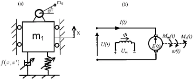
Let us consider a parametric and self-excited model, which includes a direct current (DC) motor with limited power supply, operating on a structure (Fig. 1). The excitation of the system is limited by the characteristic of the energy source (non-ideal energy source). Then, the coupling of the vibrating oscillator and the DC motor takes place. As the vibration of the mechanical system depends on the motion of the DC motor, also the motion of energy source depends on vibrations of the system. Hence, it is important to analyse what happens to the motor, as the response of the system changes.
Let us assume that the mathematical model consists of a DC motor which is supported by a non-linear spring with periodically changing stiffness of Mathieu type, and that damping of the system is described by non-linear Rayleigh’s function. These two terms guarantee coexistence of two types of vibrations in the dynamical system: parametric and self-excitation. The direct current motor, with rotating mass, is an external energy source forcing this system.
The electrical scheme of the DC motor representation is presented in Fig. 1 (b). The equations governing the motion of the DC motor are typically written in the form (Pelczynski and Krynke, 1984):
( ) ( ) ( )
2
2 m z
d
J M t M t H t dt
f
= − − (1)
( ) t ( ) t ( ) ( )
dI t U t R I t L E t
dt
= + + (2)
where: time functions U (t) and I (t) are the voltage and the current in the armature, Rt and Lt is resistance and inductance of the
armature, E(t) is the internally generated voltage, Mz(t) is an
external torque applied to the motor drive shaft, H(t) is a frictional torque and Mm(t) denotes the torque generated by the motor. The
torque Mm(t) and internal generated voltage E(t) can be expressed as
( ) ( )
m M
M t =c ΦI t (3)
( ) E ( )
E t =cΦw t (4)
where: cM, cE are mechanical and electrical constants andΦ is the
magnetic flux. Let us assume that external exciting current Im and
voltage Um are constant and then the magnetic flux Φ is also
constant in the considered model. Taking into account Eqs. (1)-(4) and mechanical model published in (Warminski et al., 2001), we can write the differential equations of the complete electro-mechanical system presented in Fig. 1 as follows:
( )
( ) ( )
t E
t t t
dI t R c U t I t
dt =−L − LΦ ′f + L
(5)
( )
( )
0 cos 0 cosM
Jf ′′=c ΦI t −H f ′ +m rx′′ f −m gr f (6)
(
)
(
)
(
3)
20 1 0
, cos2 sin o cos
mx′′+f x x′+k−k f x+k x =m rf ′ f −m rf ′′ f (7)
where a prime denotes a derivative with respect to dimensional time. The function
(
)
(
2)
1 ˆ1 ,
f x x′ = −c +c x′ x′ is called Rayleigh’s function and it describes a non-linear damping of the system. Introducing dimensionless time t =w 0t, where w 0= k m is the
natural frequency of the system and m=m1+m0, we can write
the system of differential equations (5)-(7) in a dimensionless form
( ) ( )
1 2
I=−p I t −pf+U t (8)
( ) ( )
3 2 cos
p I H q X
f= t − t − f (9)
(
2)
( )(
2)
(
2)
1
1 cos2 1 sin cos
X+−a +b X X+ −m f +g X X=q f f −f f
(10) where: 1 0 t t R p Lw
= , 2
E t zn c p L I Φ
= , 3
0 M zn c p I Jw Φ
= , 0
1 st m r q mx = , 0 2 st m rx q J = , ( ) ( ) 0 t n U U L I t t w = , ( ) ( ) 0 H H J t t w
= , 1
0 c m a w = , 2 1 0 ˆ st c x m w
b = , 2
1st k x
g = , k0
k m = ,
st x X x = , r I I I
=, and xst means
a static displacement of the system, Ir is a rated current in the
armature and dots indicate differentiations with respect to dimensionless time.
In the current literature, very often the model of DC motor is simplified (Kononenko, 1969), (Balthazar et al., 1997), by taking into account that I=0, and the moment generated by the motor can be expressed by
2 2 3
1 1
m
p p p
M U
p p w
= − . (11)
Then, a straight line approximates the characteristic of the DC motor model.
The mathematical model of the vibrating system described by Eqs. (8)-(10) can be considered in three variants:
Ideal system, if there is no coupling between motion of the rotor and vibrating system
(
2)
( )(
2)
21
1 cos 2 1 sin
X+ −a +b X X + −m w t +g X X=qw w t (12)
wheref =w t .
On the right side of equation (12), a function of time is present. non-ideal system in Kononenko’s sense
( ) q X2 cos
f=Γ t − f (13)
(
2)
( )(
2)
(
2)
1
1 cos 2 1 sin cos
X+−a +b X X+ −m f +g X X=q f f −f f
(14)
whereΓ
( )
f =Mm( )
f −H( )
f is the difference between the torque generated by the motor and the resistance torque. Function( )
f u1 u2fΓ = − is approximated by a straight line, whereu1 is a
control parameter and it can be changed according to the voltage,
2
u is a constant parameter, characteristic for the model of the motor.
Full non-ideal electro-mechanical system described by Eqs. (8)-(10).
All above three models describe the same problem in different simplification levels. However, they may lead to qualitative and quantitative differences in their behaviours. The comparison of the results obtained for ideal and non-ideal problems and for different of DC motor models are presented in the next section.
Analysis of the Vibrating System in Different Simplification Levels
1 2 3
1 2
0.3, 3.0, 0.15, 0.1, 0.05, 0.1,
0.2, 0.2, 0.3
p p p
q q
a b g
m
= = = = = =
= = =
(15)
In the ideal model described by (12), the external force is expressed on the right side of the differential equation by a pure function of time. Analysis for this ideal problem was carried out in details in (Szabelski and Warminski, 1995a, b).
0.9 0.95 1 1.05 1.1 1.15
ω 0
0.4 0.8 1.2 1.6
a
(a)
0.9 1 1.1 1.2
ω 0
0.5 1 1.5 2 2.5
a
(b)
Figure 2. Amplitude curves around the main parametric resonance for the ideal system, (a) without an external forceαα = 0.01,ββ = 0.05,γγ = 0.1,
µµ = 0.2,q1 = 0, and (b) for the system forced by ideal harmonic function
αα = 0.1, ββ = 0.05, γγ = 0.1, µµ = 0.2, q1 = 0.2.
If the external force is not present (q1=0) then the resonance
curve has the shape presented in Fig.2 (a). Interaction between parametric and self-excited system leads to the synchronisation phenomenon near the main parametric resonance. In this region, parametric vibrations dominate. They pull in the frequency of self-excited vibrations and the system vibrates with a single frequency and with a constant amplitude (solid line in Fig.2 (a)). Outside the synchronisation regions, influence of the self-excitation is bigger and two frequencies in the response of the system occurs. System vibrates periodically and its motion is visible as a quasi-periodic limit cycle on the phase plane (see details Szabelski and Warminski, (1995 a,b) ). Vertical lines in Fig.2 (a), which denote maximal and minimal values of the modulated amplitude, mark this motion.
The external force causes very important qualitative changes. Behaviour of the ideal system for q1=0.2is presented in Fig.2 (b).
Additional solutions, having a shape of an internal loop, appear in the synchronisation region. However only the upper part of this loop is stable.
Figure 3. Amplitude curves versus parameter q1.
The shape of the resonance curve depends on the value of the amplitude of the external excitation. The internal loop is visible only for small level of the external excitation. For large value of theq1
parameter, the loop disappears (Fig.3).
0.8 1.2 1.6 2 2.4 2.8 3.2 3.6 4
u1
0 0.5 1 1.5 2 2.5 3
a
(a)
0.8 1.2 1.6 2 2.4 2.8 3.2 3.6 4
u1
0 0.5 1 1.5 2 2.5 3
Ω
(b)
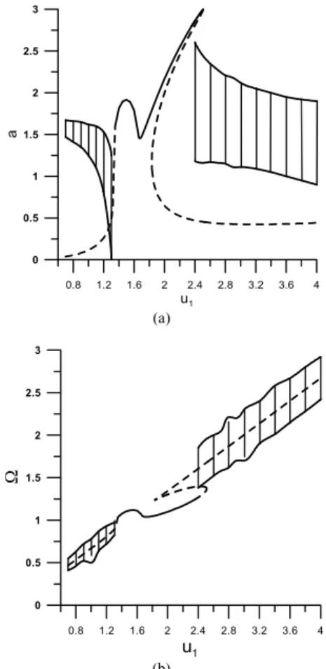
Figure 4. Amplitude of vibrating oscillator and angular velocity of the motor versus control parameter u1.
q1=
q1
ω
ω
a
q1
q1
q1
If we assume that the system is forced by a DC motor with limited power, then it is necessary to consider its dynamics in the model and to solve the system of differential equations (13)-(14). The torque generated by DC motor is limited and, according to classical Kononenko theory, is assumed as a straight line. Transition through the resonance region is possible if the parameter u1, connected with voltage supplied to the motor, is increased. The vibration amplitude of the oscillator and the angular velocity of the rotor are presented in Fig.4.
0.4 0.8 1.2 1.6 2 2.4 2.8
Ω
0 0.5 1 1.5 2 2.5 3
a
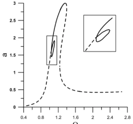
Figure 5. Amplitude versus angular velocity of the motor.
Outside the synchronisation region the oscillator vibrates periodically and the motor angular velocity changes have quasi-periodic character as well (vertical lines in Fig.4). Inside the synchronisation area the motion of the system is periodic (solid line in Fig.4). During transition through this resonance, local decreasing of the amplitude and angular velocity takes place. This phenomenon affects the resonance curve, amplitude versus excitation frequency (Fig.5). On the resonance curve, an internal loop is visible, however its lies on the left branch of the curve and is completely stable. Analytical solutions and stability analysis have been carried out in (Warminski et al., 2001).
Time histories of the vibration of the oscillator and the variation of the angular velocity of DC motor are presented in Fig.6. In Fig.6 (b), the system vibrates with the constant amplitude while, in Fig.6 (a), (c), (d) the motion is quasi-periodic.
The most adequate model to the realistic problem is described by electro-mechanical equations (8)-(10). To simulate the mathematical model of this system, MATLAB, SimulinkTM and
Dynamics package (Nusse and York, 1998) were applied. Differential equations were solved by fifth order Runge-Kutta method with automatic step length and integration error control. Behaviour of the system was observed during slow voltage increasing, and then vibration amplitude of the oscillator and angular velocity of the motor were plotted.
0 100 200 300 400 500
t -1.4
-1.2 -1 -0.8 -0.6 -0.4 -0.2 0 0.2 0.4 0.6 0.8 1 1.2 1.4
X
,
ω
(a)
0 40 80 120 160 200
t
-2.4 -2 -1.6 -1.2 -0.8 -0.4 0 0.4 0.8 1.2 1.6 2 2.4
X
,
ω
(b)
0 40 80 120 160 200
t
-2.4 -2 -1.6 -1.2 -0.8 -0.4 0 0.4 0.8 1.2 1.6 2 2.4
X
,
ω
(c)
0 40 80 120 160 200
t
-2.4 -2 -1.6 -1.2 -0.8 -0.4 0 0.4 0.8 1.2 1.6 2 2.4
X
,
ω
(d)
Figure 6. Times histories for non-ideal system and chosen control parametersu1; (a) u1=1.30, (b) u1=2.20, (c) u1=2.40, (d) u1=2.80.
ω
0 200 400 600 800 1000
t
-2.5 -2 -1.5 -1 -0.5 0 0.5 1 1.5 2 2.5
X
,
ω
1 2 U 3 4 5
(a)
0 200 400 600 800 1000
t
-2.5 -2 -1.5 -1 -0.5 0 0.5 1 1.5 2 2.5
X
,
ω
1 2 3 4 5
U
(b)
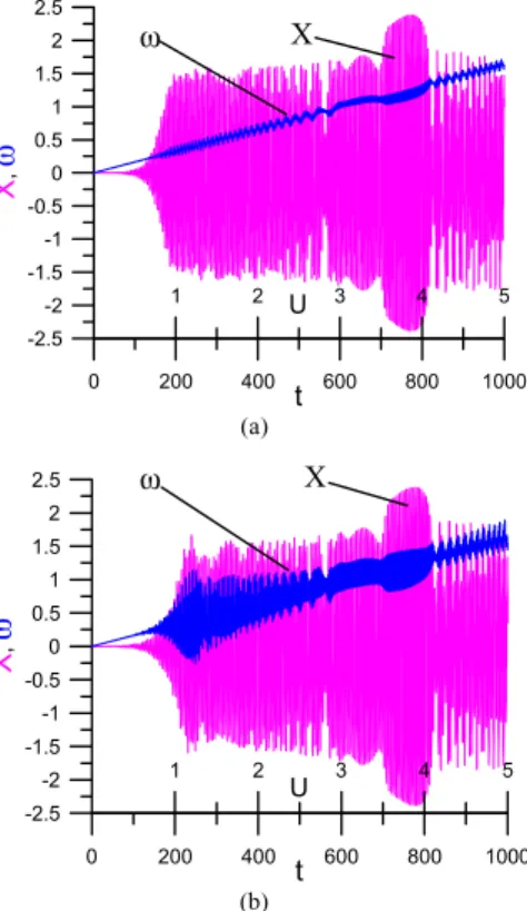
Figure.7. Displacement of the oscillator and angular velocity of the shaft versus control parameter U and versus dimensionless time near the main parametric resonance, simplified (a) and complete (b) model of DC motor.
The dimensionless voltage applied across the armature
( )
( )
0, 5U t ∈ is the control parameter. In Fig. 7 we can compare results obtained for two different models of a non-ideal problem. The model simplified in Kononenko sense is limited by influence of the DC motor characteristic described by the Eq. (11). The stationary characteristic of the motor, for assumed data (15), is expressed by the function Γ
( )
f =1.83−5.57f. Transition through resonance for this model is presented in Fig. 7(a). The results for the complete electro-mechanical model described by the full system of differential equations (8)-(10) are presented in Fig.7 (b). Transition through the main parametric resonance takes place for voltage near( )
3, 4U∈ and for time t ∈
(
600, 800)
. Comparing Fig. 7 (a) and (b), we can find that the motions of the oscillator X have similar character. Near U=3.5, in both figures, local decreasing of vibration amplitude of the oscillator is visible. Transformations of Figs.7 (a) and (b) to the dependence a( )Ω i.e. the amplitude versus angular velocity curve, lead to the loop presented in Fig.5. The important difference occurs in DC motor dynamics. The changes of angular velocity ω are much more complex for the complete electro-mechanical model (Fig.7(b) ) than for the simplified non-ideal model (Fig.7(a) ).(a)
(b)
Figure 8. Lyapunov exponents diagram versus control parameter U, simplified (a) and complete (b) DC motor model, regular motion (µµ=0.2).
(a)
(b)
Figure 9. Lyapunov exponents diagram versus control parameter U, simplified (a) and complete (b) DC motor model, chaotic regions (µµ=1.0).
ω X
If we compare Lyapunov exponents diagrams obtained for the same parameters (Fig. 8), we see that for the considered interval of the control parameter, the motion of the system is regular; Lyapunov exponents are negative or equal to zero. Nevertheless, we can notice that around the intervals nearU=1.0 andU∈(3, 4), behaviour of the system in the diagram Fig. 8 (b) is more complex. It confirms results presented in Fig. 7(b).
For the ideal system (Eq. (12)) and for a wide range of parameters used, it was not possible to find chaotic motion of the model. The ideal system vibrates regularly, periodically or quasi-periodically (Szabelski and Warminski, 1995 a,b). For non-ideal model, based on the paper (Warminski, 2001b), we can expect that the increase of the parametric excitation can lead to chaotic motion. Therefore, let us assume for both considered non-ideal models, that the parametric excitation isµ=1.0. Lyapunov exponents diagram for that case is plotted in Fig. 9.
We see that in a few intervals of the control parameter U, maximal Lyapunov exponent has a positive sign. However, the tendency in transition to chaotic motion is different. Chaotic motion for the full electro-mechanical model (Fig. 9(b)) appears in a wider region, in opposition to the simplified model (Kononenko approach) for which chaotic motion appears only for a few small regions.
(a)
(b)
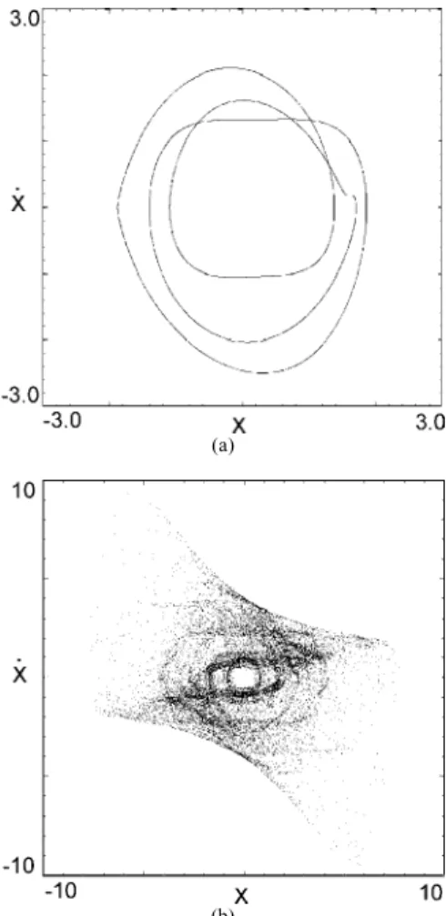
Figure 10. Poincaré diagrams for equivalent DC motor models, regular attractor for simplified model (a) and strange chaotic attractor for complete model (b), µµ=1.0, U=2.0.
Poincaré diagrams for equivalent parameters and different non-ideal models are presented in Fig. 10. The motion of the simplified
model is regular and it is represented by a closed orbit in Fig.10(a), with Lyapunov exponents l 1=0,l 2=−0, 007,
3 0.106, 4 5.739
l =− l =− , whilst the motion of the complete model for the same parameters, is chaotic. In Fig. 10(b) the chaotic attractor with one Lyapunov’s exponent positive is presented
(l 1=0.077,l 2 =0,l 3=−0.159, l 4=−0.348, l 5=−0.516).
This result shows that the difference in dynamic behaviour for different models is significant, particularly for regions where chaotic motion is possible.
Remarks and Conclusions
Analysis carried out in this paper emphasizes differences in modeling of ideal and non-ideal systems for a chosen class of self-, parametric and externally excited vibrations. Behaviours of the ideal and non-ideal system are different. The external force generated by the ideal motor introduces additional solutions in the synchronisation region. These solutions are observed as an internal loop inside the resonance curve with only the upper part stable. However if the parametric and self-excited system is forced by a non-ideal energy source, the loop moves to the left branch of the curve and becomes stable.
The obtained results let us also conclude that two different approaches to the modeling of non-ideal systems can lead to important differences. The classical model proposed by Kononenko (1969) is based on the pure mechanical model of the DC motor and takes into account the stationary characteristic of the energy source. That approach considers only mechanical interactions between the oscillating system and the energy source, which is limited by an assumed straight line. To be close to the realistic system, the model should take into account also influence of the dynamics of the oscillating mechanical elements on electrical properties of the DC motor. Therefore, two alternative models were analysed in this paper: the simplified classical model and the complete electro-mechanical model. Numerical simulations show that for regular motion, and for slow transition through the resonance region, behaviour of two considered models is similar. Nevertheless, if the dynamics of the systems becomes complex, then the difference in the response of those two models is more significant. Transition from regular motion to chaos is possible for both models. However, the tendency in going to chaos for the electro-mechanical model is bigger. The general conclusion is that simplified model attenuates dynamics of the realistic system. For example, if the chaotic region is found for the simplified model, we can expect that for the complete electro-mechanical model chaotic motion will appear in a much wider area. The opposite situation was not observed.
References
Awrejcewicz, J. and Mrozowski, J., 1989, “Bifurcation and Chaos of a Particular Van der Pol-Duffing's Oscillator”, Journal of Sound and Vibration, 132 (1), pp. 89-100.
Balthazar, J.M., Rente, M.L. and Davi, V.M., 1997, “Some Remarks On the Behaviour of a Non-Ideal Dynamical System”, in Nonlinear Dynamics, Chaos, Control and Their Applications to Engineering Sciences, eds. Balthazar, J.M., Mook, D.T. & Rosario, J.M. (American Academy of Mechanics and Associacao Brasileira de Ciencias Mecanicas) Vol. 1, pp. 97-104.
Belato, D., Weber, H.I., Balthazar J.M. and Mook, D.T., 2001, “Chaotic Vibrations of a Nonideal Electro-Mechanical System”, Int. Journal of Solids and Structures, 38, pp.1699-1706.
Kononenko, V.O., 1969, Vibrating Systems with Limited Power Supply, Illife.
Pe³czyñski, W., and Krynke, M., 1984, Method of State Variables in Analysis of Power Transmission System Dynamics, WNT, Warsaw, Poland, (in Polish).
Pontes, B.R., Oliveira, V.A. and Balthazar, J.M., 2000, “On Friction-Driven Vibrations in a Mass-Block-Motor System with a Limited Power Supply”, Journal of Sound and Vibration, 234(4), pp. 713-723, doi:10.1006/jsvi.2000.2882.
Szabelski, K. and Warminski, J., 1995 a, “The parametric self excited non-linear system vibrations analysis with the inertial excitation”, Int. Journal of Non-Linear Mechanics Vol.30, No 2, pp. 179-189.
Szabelski, K. and Warminski, J., 1995 b, “The self-excited system vibrations with the parametric and external excitations”, Journal of Sound and Vibration, 187 (4) pp. 595-607.
Tondl, A. and Ecker, H., 1999, “Cancelling of Self-Excited Vibrations by Means of Parametric Excitation”, Proceedings of the 1999 ASME Design Engineering Technical Conferences, September 12-15, Las Vegas, Nevada, USA, DETC99/VIB-8071, pp. 1-9.
Warminski, J., Balthazar, J.M. and Brasil, R.M.L.R.F., 2001, “Vibrations of Non-Ideal Parametrically and Self-Excited Model”, Journal of Sound and Vibration, 245 (2), pp. 363-374, doi:10.1006/jsvi.2000.3515.
Warminski, J., 2001a, “Influence of the External Force on the Parametric and Self-Excited System”, Journal of Technical Physics, 42, pp. 349-366.
Warminski, J., 2001b, “Synchronisation Effects and Chaos in van der Pol-Mathieu Oscillator”, Journal of Theoretical and Applied Mechanics, 4, 39, pp. 1-24.
Warminski, J., 2001c, “Regular and Chaotic Vibrations of Parametrically and Self-Excited Systems with Ideal and Non-Ideal Energy Sources”, Technical University of Lublin Publisher, Lublin, Poland, (in Polish).