Volcano impacts on climate and biogeochemistry in a coupled carbon-climate model

(1)

ESDD

3, 279–323, 2012

Volcano impacts on climate and biogeochemistry

D. Rothenberg et al.

Title Page

Abstract Introduction

Conclusions References

Tables Figures

◭ ◮

Back Close

Full Screen / Esc

Printer-friendly Version Interactive Discussion

Discussion

P

a

per

|

Dis

cussion

P

a

per

|

Discussion

P

a

per

|

Discussio

n

P

a

per

|

Earth Syst. Dynam. Discuss., 3, 279–323, 2012 www.earth-syst-dynam-discuss.net/3/279/2012/ doi:10.5194/esdd-3-279-2012

Earth System Dynamics Discussions

This discussion paper is/has been under review for the journal Earth System Dynamics (ESD). Please refer to the corresponding final paper in ESD if available.

Volcano impacts on climate and

biogeochemistry in a coupled

carbon-climate model

D. Rothenberg1,*, N. Mahowald1, K. Lindsay3, S. C. Doney4, J. K. Moore5, and P. Thornton6

1

Department of Earth and Atmospheric Sciences, Cornell University, Ithaca, NY 14853, USA 3

Climate and Global Dynamics Division, National Center for Atmospheric Research, Boulder, CO 80305, USA

4

Department of Marine Chemistry and Geochemistry, Woods Hole Oceanographic Institution, Woods Hole, MA 02543, USA

5

Department of Earth System Science, University of California, Irvine, CA 92697, USA 6

Environmental Sciences Division, Oak Ridge National Laboratory, Oak Ridge, TN 37831, USA

*

now at: Department of Earth, Atmospheric, and Planetary Sciences, Massachusetts Institute of Technology, Cambridge, MA 02139, USA

Received: 21 March 2012 – Accepted: 26 March 2012 – Published: 18 April 2012 Correspondence to: D. Rothenberg ([email protected])

(2)

ESDD

3, 279–323, 2012

Title Page

Tables Figures

◭ ◮

Back Close

Full Screen / Esc

Discussion

P

a

per

|

Dis

cussion

P

a

per

|

Discussion

P

a

per

|

Discussio

n

P

a

per

|

Abstract

Volcanic eruptions induce a dynamical response in the climate system characterized by short-term, global reductions in both surface temperature and precipitation, as well as a response in biogeochemistry. The available observations of these responses to volcanic eruptions, such as to Pinatubo, provide a valuable method to compare against 5

model simulations. Here, the Community Climate System Model Version 3 (CCSM3) reproduces the physical climate response to volcanic eruptions in a realistic way, as compared to direct observations from the 1991 eruption of Mount Pinatubo. The model biogeochemical response to eruptions is smaller in magnitude than observed, but be-cause of the lack observations, it is not clear why or where the modeled carbon re-10

sponse is not strong enough. Comparison to other models suggests that this model response is much weaker in the tropical land; however the precipitation response in other models is not accurate, suggesting that other models could be getting the right response for the wrong reason. The underestimated carbon response in the model compared to observations could also be due to the ash and lava input of biogeochem-15

ical important species to the ocean, which are not included in the simulation. A statis-tically significant reduction in the simulated carbon dioxide growth rate is seen at the 90 % level in the average of 12 large eruptions over the period 1870–2000, and the net uptake of carbon is primarily concentrated in the tropics with large spatial variability. In addition, a method for computing the volcanic response in model output without using 20

a control ensemble is tested against a traditional methodology using two separate en-sembles of runs; the method is found to produce similar results. These results suggest that not only is simulating volcanoes a good test of coupled carbon-climate models, but also that this test can be performed without a control simulation in cases where it is not practical to run separate ensembles with and without volcanic eruptions.

(3)

ESDD

3, 279–323, 2012

Title Page

Tables Figures

◭ ◮

Back Close

Full Screen / Esc

Discussion

P

a

per

|

Dis

cussion

P

a

per

|

Discussion

P

a

per

|

Discussio

n

P

a

per

|

1 Introduction

Volcanic eruptions provide sharp, transient, and relatively well-understood forcings to the climate system, and induce short-term global surface cooling and lower-stratospheric warming in their aftermath (Mass and Portman, 1989; Robock and Mao, 1992, 1995; Shindell et al., 2004). This response is due to the eruptions’ injection of 5

large amounts of sulfate aerosols into the stratosphere, which increases the amount of incoming solar radiation reflected back out to space at the top of the atmosphere. Although stratospheric aerosols tend to mix relatively quickly in the atmosphere (less than a few months), tropical eruptions tend to have greater climate impacts than high-latitude ones, due to both longer residence times of their aerosols as well as an appar-10

ent stronger dynamic response (Oman et al., 2005).

The forcing from volcanic eruptions tends to cool the tropics but produces some continental warming in the winter, similar in spatial pattern to a shift towards the positive phase of the Arctic Oscillation in the Northern Hemisphere (Stenchikov et al., 2006; Oman et al., 2005; Shindell et al., 2004). It has also been observed in the paleoclimate 15

record that a multi-year, El Ni ˜no-like response can be induced in the atmosphere-ocean system as a response to explosive, tropical volcanic eruptions (Adams et al., 2003).

Because of their strong impacts on climate, volcanic eruptions provide good natural experiments to test the sensitivity of climate models. Very large volcanic explosions ap-pear to increase the likelhood of an El Ni ˜no event (Emile-Geay et al., 2008). Stenchikov 20

et al. (2006) analyzed the IPCC AR4 climate models and showed that although the included models reproduced a post-eruption shift to the positive phase of the Arctic Oscillation, there was considerable spread in the set of models’ particular dynamic responses. Furthermore, the winter warming of the continents in the Northern Hemi-sphere (associated with a shift to the positive phase of the AO) was much weaker in 25

(4)

ESDD

3, 279–323, 2012

Title Page

Tables Figures

◭ ◮

Back Close

Full Screen / Esc

Discussion

P

a

per

|

Dis

cussion

P

a

per

|

Discussion

P

a

per

|

Discussio

n

P

a

per

|

following eruptions, contrary to the response identified by Adams et al. (2003) in the paleoclimate record.

Direct observations of the 1991 Mount Pinatubo eruption provide a baseline for an-alyzing models’ physical climate responses to volcanoes. While the Pinatubo eruption

produced global surface cooling of about 0.5◦C (Hansen et al., 1996), it yielded strong

5

continental warming in the Northern Hemisphere winter following the eruption (Shin-dell et al., 2004). Precipitation over land was strongly diminished in the aftermath of Pinatubo as well, especially in Europe and in the tropics in South America and Africa (Trenberth and Dai, 2007).

The surface cooling, increase in diffuse radiation, and global precipitation reduction

10

following eruptions have impacts on the carbon cycle. In 1991, the growth rate of

atmo-spheric CO2 was expected to rise due to the onset of an El Ni ˜no, but in the aftermath

of the Pinatubo eruption, the growth rate reversed signs and atmospheric CO2 levels

dropped slightly (Sarmiento, 1993). This Pinatubo-CO₂anomaly was potentially linked

to a connection between post-eruption global cooling and a resulting shift in the be-15

havior of the terrestrial biosphere. However, it is difficult to directly ascribe variability in

atmospheric CO₂to volcanic eruptions because inter-annual variability in atmospheric

CO2 is closely tied to the El Ni ˜no-Southern Oscillation (ENSO) (Jones et al., 2001).

During periods of El Ni ˜no, the terrestrial biosphere becomes a net source of CO2to the

atmosphere, whereas the opposite trends occurs during La Ni ˜na events (Jones et al., 20

2001); thus deconvolving the effects of volcanoes from El Ni ˜no events is difficult.

Ob-servational evidence is too limited to diagnose from observations what is driving the carbon response. Tree ring records suggest that in some temperate forests, net pri-mary production is reduced due to volcano-induced cooling (Krakauer and Randerson, 2003). A transient reduction in net primary production in the high latitudes following 25

Pinatubo has been attributed to decreased growing-season length due to volcanic-induced cooling (Nemani et al., 2003). However, some low-latitude ecosystems expe-rienced increased plant growth as cooling reduced evaporative demand or volcanic

(5)

ESDD

3, 279–323, 2012

Title Page

Tables Figures

◭ ◮

Back Close

Full Screen / Esc

Discussion

P

a

per

|

Dis

cussion

P

a

per

|

Discussion

P

a

per

|

Discussio

n

P

a

per

|

North America during 1992–1993 as compared to previous time periods has also been observed (Bousquet et al., 2000).

The ocean response to volcanoes is not well documented. Some authors argue that the additional nutrients and trace elements added to the ocean may be responsible for additional carbon uptake (e.g., Watson, 1997; Frogner et al., June, 2001; Duggen 5

et al., 2007, 2010), but a quantative assessment of this effect on global carbon or

ocean productivity has not yet been performed. The strength of land and ocean sinks

of CO₂are not increasing along with rising anthropogenic emissions (Le Qu ´er ´e et al.,

2009; Sarmiento et al., 2010) as evidenced by an increase in atmospheric CO2levels.

Modeling studies suggest that the balance of increased carbon uptake associated with 10

CO₂ fertilization and decreased uptake associated with global warming could lead to

a reduction in the efficiency of the land sink of carbon in the future (Cox et al., 2000;

Friedlingstein et al., 2006; Thornton et al., 2009; Sitch et al., 2008). Studies of future carbon dioxide levels tend to use sophisticated coupled-carbon cycle models and one

of the difficulties with these models is finding ways to test their response to climate

15

change. The carbon cycle response to volcanoes is a valuable testing metric (Jones and Cox, 2001; Friedlingstein and Prentice, 2010).

This study investigates the performance of one coupled-carbon-climate model – the CCSM3 (Thornton et al., 2009; Mahowald et al., 2011) – by analyzing the responses by the ocean and land carbon cycle to volcanic eruptions during the period 1870– 20

2000. This study di_ffers from previous studies in several ways: it looks at multiple

vol-canoes over 130 yr, while Jones and Cox (2001) focused on the volcanic forcing of

climate and the impact on the carbon cycle using a different model and only for the

Pinatubo eruption, while Brovkin et al. (2010) looked at the role of eruptions over the last 1000 yr. In addition, this study compares the response using a control case (with-25

(6)

ESDD

3, 279–323, 2012

Title Page

Tables Figures

◭ ◮

Back Close

Full Screen / Esc

Discussion

P

a

per

|

Dis

cussion

P

a

per

|

Discussion

P

a

per

|

Discussio

n

P

a

per

|

http://cmip-pcmdi.llnl.gov/cmip5/). It also indicates what fraction of the true volcano signal we expect to see in the real world, where we have no control case. Previous studies at higher resolution with the CCSM3 suggest that the model is able to capture

the observed response to volcanoes (Schneider et al., 2009), but generally has diffi

-culty in accurately capturing El Ni ˜no (Deser et al., 2006). This paper, similar to Jones 5

and Cox (2001), does not consider the potentially important impacts of the addition of biogeochemically relevant species with the volcanic eruption, but only the response to the physical forcing. Section 2 describes the model configuration and experimental setup for the simulations in these studies. Section 3 describes the results, and Sect. 4 summarizes and discusses the implications of this study.

10

2 Methods

2.1 Model description

The model used here is based on the NCAR Community Climate System Model, Ver-sion 3 (CCSM3) as described in Collins et al. (2006a) and Yeager et al. (2006) and is run in a coupled configuration with atmosphere, land, ocean, and sea ice components 15

with the addition of a fully-coupled carbon cycle with land and ocean components, as described in Thornton et al. (2009) and Mahowald et al. (2011). The model was config-ured identically to the one used in the aerosol experiments in Mahowald et al. (2011),

with the CAM atmosphere model component running at a T31 resolution (3.75◦×3.75◦

latitude-longitude grid) with 26 vertical levels (Collins et al., 2006b); it included esti-20

mates of historical volcanic forcing, as well as prognostic carbonaceous, sulfate, dust and sea salt aerosols and corresponding emissions varying over the time period 1870– 2000 (Meehl et al., 2006). The time-varying volcanic forcing dataset used here, as well as in Meehl et al. (2006), derives from previous work by Ammann et al. (2003).

Ammann et al. (2003) scaled the peak aerosol depth for 20th century eruptions 25

(7)

ESDD

3, 279–323, 2012

Title Page

Tables Figures

◭ ◮

Back Close

Full Screen / Esc

Discussion

P

a

per

|

Dis

cussion

P

a

per

|

Discussion

P

a

per

|

Discussio

n

P

a

per

|

composition of 75 % H₂SO₄ and 25 % H₂O and fixed aerosol size distribution (with

r_e_ff=0.42 micron). This is comparable to the composition of Pinatubo’s aerosols

(Am-mann et al., 2003). Immediately following the month of the eruption, the aerosols build up linearly in the lower stratosphere (150 to 50 hPa) for four months before reaching the estimated peak load of sulfate aerosol. In the forcing dataset, aerosols are removed at 5

the poles during winter, and the e-folding time for their decay in the tropics is 12 months (Ammann et al., 2003). Ammann et al. (2003) suggest that their parametrization for the post-eruption atmospheric aerosol loading successfully reproduces the timing and hemispheric evolution of aerosol spread except for the eruptions of Agung in 1963 and El Chichon in 1982. Following the Agung eruption, the model used by Ammann et al. 10

(2003) overestimated the amount of aerosol transported to the Northern Hemisphere, whereas following the eruption of El Chichon, more aerosols were observed in the Northern Hemisphere than the model predicted.

The land carbon cycle used in these simulations (CLM-CN) includes linked carbon and nitrogen cycles (Thornton et al., 2007). The land biogeochemistry in this model in-15

cludes N-limitation, which reduces carbon uptake in the presence of higher CO2

condi-tions (Thornton et al., 2007). The CLM-CN has been previously evaluated for its mean behavior by Randerson et al. (2009). Ocean biogeochemistry is handled here with the Biogeochemical Element Cycling model (Moore et al., 2004), which includes a full depth carbon-cycle module, and has been compared against available observations by 20

Doney et al. (2009a,b). The BEC model also features several phytoplankton functional groups (including diazotrophs, diatoms, and smaller phytoplankton) and growth-limiting nutrients (nitrate, phosphate, iron, and others) (Thornton et al., 2009).

The CCSM3 also includes a module modeling sources, atmospheric transport, and deposition of desert dust, as described by Zender et al. (2003) and Mahowald et al. 25

(2006). The dust model generates dust in regions with un-vegetated, dry soils with strong winds and easily erodible soil (Zender et al., 2003). Interactions between the dust and ocean biogeochemistry modules has previously been investigated (Mahowald

(8)

ESDD

3, 279–323, 2012

Title Page

Tables Figures

◭ ◮

Back Close

Full Screen / Esc

Discussion

P

a

per

|

Dis

cussion

P

a

per

|

Discussion

P

a

per

|

Discussio

n

P

a

per

|

limitation of nitrogen fixing organisms and ultimately impacts oceanic uptake of carbon dioxide in the model.

Ensemble member setup

Model runs were branched from a control run after 50 yr and subsequently integrated over a 130-yr period spanning 1870–2000, as described in more detail in Mahowald 5

et al. (2011). In addition to the “AEROSOL” simulation referred to in that paper, two additional ensemble members with volcanoes were setup and integrated for this study, and branched from points set ten years apart. Another ensemble of three branched simulations was computed here, but with volcanoes disabled for the entire period of integration (control simulations).

10

2.2 Volcanic eruptions

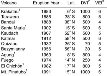
A selection of eruptions (see Table 1) was made based on Robock and Mao (1992), and adjusted to facilitate comparison to other papers by choosing only the most commonly analyzed eruptions (Jones and Cox, 2001; Robock and Liu, 1994; Shindell et al., 2004; Oman et al., 2005; Stenchikov et al., 2006; Schneider et al., 2009). Robock and Mao 15

(1992) chose eruptions (Table 1) occurring between 1870–2000 which satisfied the

criteria of VEI (volcanic explosivity index) ≥5 or DVI (dust veil index) ≥250. These

criteria were chosen to maximize the potential climate impacts of each eruption; large VEI’s correspond to eruptions emitting a large volume of tephra in a tall eruption cloud, and large DVI’s are associated with a large release of dust and aerosols that impact 20

the Earth’s radiative balance during the years immediately following an eruption. The combination of high VEI and DVI help to maximize a volcano’s impact on Earth’s energy balance, yielding a more visible signal in the climate record (via short-term surface cooling). The analyses presented in this study were performed with the subset of these eruptions indicated in Table 1. Because the eruptions compiled by Robock and Mao 25

(9)

ESDD

3, 279–323, 2012

Title Page

Tables Figures

◭ ◮

Back Close

Full Screen / Esc

Discussion

P

a

per

|

Dis

cussion

P

a

per

|

Discussion

P

a

per

|

Discussio

n

P

a

per

|

in various seasons, the response to eruptions tends to be averaged out when all the eruptions are included in the analysis performed here. The subset of five eruptions – Krakatau, Santa Maria, Agung, El Chichon, and Pinatubo – was chosen by taking the largest tropical eruptions which yielded the most significant physical climate response.

2.3 Model and data analysis

5

2.3.1 Timeseries

Trends in the climate record immediately following volcanic eruptions were computed by analyzing timeseries of anomalies between paired ensemble members – one which included volcanoes and a matched control. Four-year timeseries were composited starting at the month of each eruption for each model run in the two ensembles; the 10

timeseries were separated into a group with eruptions and a control without. For each

month, the mean and standard deviation for the difference between the eruption and

control samples was computed. This mean anomaly between volcanic runs and con-trol runs was compared to the set of anomaly timeseries for each individual eruption, averaged over the three pairs (volcano-control) of ensemble members.

15

In addition, a second anomaly was computed without making reference to the con-trol simulations (“no-concon-trol” case) by analyzing deviations from the average seasonal cycle immediately preceding each eruption. For each month in the years following the eruption, an anomaly is computed based on the two years previous to the eruption to compute the deviation from the average seasonal cycle. To compute the ‘no-control’ 20

anomaly for atmospheric CO2 following Pinatubo, a similar procedure was used but

the data was de-trended before computing the seasonal cycle to facilitate comparisons between the data before and after the eruption; in order to detrend the data, a linear regression was performed on a 20 yr period centered at the eruption and subtracted from the simulation timeseries.

(10)

ESDD

3, 279–323, 2012

Title Page

Tables Figures

◭ ◮

Back Close

Full Screen / Esc

Discussion

P

a

per

|

Dis

cussion

P

a

per

|

Discussion

P

a

per

|

Discussio

n

P

a

per

|

2.3.2 Pinatubo

Jones et al. (2001) performed an ensemble of 9 runs with the HadCM3 over the time

period 1990 to 1996 to investigate effect of the Pinatubo eruption on the dynamics of

the climate and biogeochemistry. They compared surface temperature observations to model-computed temperatures, and analyzed the components of the model contribut-5

ing to the terrestrial biosphere’s uptake of CO2 over the duration of the model runs.

Similar analyses were performed here to compare the CCSM3’s performance to the HadCM3, by analyzing the ensemble of 3 paired runs over equivalent time periods and computing both the “volcano-control” and “no-control” anomalies as previously de-scribed.

10

2.3.3 Global analyses

To analyze spatial patterns in the response to volcanic eruptions, seasonally-averaged anomalies were computed using each of the methods described in the previous section at each latitude-longitude grid point by taking the average anomaly for each individual eruption and averaging them over the subset of five eruptions. For the “volcano-control” 15

anomalies, statistical significance was computed by performing a Student’s t-test to

test whether the mean difference between the set of volcano data and control data at a

given grid point over the time period being averaged was different at a significance level

of 90 %. For the “no-control” anomalies, a one-sample Student’s t-test was used to test

whether the mean of the anomalies was significantly different from 0 at a significance

20

(11)

ESDD

3, 279–323, 2012

Title Page

Tables Figures

◭ ◮

Back Close

Full Screen / Esc

Discussion

P

a

per

|

Dis

cussion

P

a

per

|

Discussion

P

a

per

|

Discussio

n

P

a

per

|

3 Results

3.1 Physical climate response to volcanic forcing

The CCSM3’s dynamical response to volcanic forcing has previously been investigated at higher spatial resolution, but uncoupled to the carbon cycle (Schneider et al., 2009), and there is a great deal of analysis available on the larger eruptions of the past cen-5

tury for other models (Shindell et al., 2004; Robock and Mao, 1995; Stenchikov et al., 2006). In the global average, we expect to see cooling after major eruptions due to the negative radiative forcing of the aerosol particles emitted by the volcano and

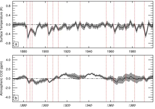
subse-quently dispersed. Here, global surface temperatures drop between 0.4 and 0.8◦C for

a short period of time following some eruptions (Fig. 1a); these largest modeleded re-10

sponses occur after three of the four largest eruptions studied here – Krakatau (1883), Santa Maria (1902), and Pinatubo (1991). All of these eruptions had VEI’s of 6, and occurred in the tropics.

In response to the Pinatubo eruption in particular, the model here produces transient

surface cooling of about 0.5◦lobal average, similar to observations (Fig. 2a), regardless

15

of the method chosen to compute the anomalies. The average cold season (October– arch) surface temperature response to all 12 eruptions in Table 1 (Fig. 3a) is also similar to observations (Shindell et al., 2004) when using the “volcano-control” method to compute the anomalies. However, the “no-control” anomalies fail to capture the spa-tial patterns in the response seen in observations – weak cooling across much of the 20

globe, with strong cooling in the high latitudes over North America and warming in the high latitudes over Europe and Asia (Shindell et al., 2004). Factors such as the state of

ENSO could be a source of variability contributing to differences between the modeled

and observed response here; the model here does not well simulate ENSO (Collins

et al., 2006b), and the phase of ENSO in the fully coupled simulations here di_ffers with

25

observations.

(12)

ESDD

3, 279–323, 2012

Title Page

Tables Figures

◭ ◮

Back Close

Full Screen / Esc

Discussion

P

a

per

|

Dis

cussion

P

a

per

|

Discussion

P

a

per

|

Discussio

n

P

a

per

|

dries in much of the tropics over land. However, the model does not respond as strongly in either wetting or drying as compared to observations (Trenberth and Dai, 2007). The precipitation response over the oceans was not analyzed by Trenberth and Dai

(2007), but they are shown here to highlight differences between the two anomaly

methods used in this study. The “no-control” anomaly method (Fig. 4b) produces a 5

weaker response over land as opposed to over the ocean, and tends to shift the strong drying responses over South America and sub-Saharan Africa seen in the “volcano-control” anomalies (Fig. 4b) towards the oceans bordering these regions to the West.

Averages over the regions of strong surface temperature and precipitation responses

(Fig. 5) emphasize the differences between the “volcano-control” and “no-control”

10

anomalies. The surface temperature response (Fig. 5a) di_ffers primarily in Europe

and the high latitudes, where the particular spatial pattern juxtaposition of strong cool-ing and strong warmcool-ing changes dependcool-ing on the anomaly method used. The large

di_fferences in the precipitation response (Fig. 5b) manifest as greater uncertainty in

the regionally-averaged response for the “no-control” anomalies as compared to the 15

“volcano-control” ones. Furthermore, the regionally-averaged responses in precipita-tion to Pinatubo tend to be larger in magnitude than the globally-averaged response because weak responses outside of these regions tends to diminish the magnitude

of the globally-averaged response. These regional differences, though, might also be

influenced by the phase of ENSO and other variability between ensemble members, 20

and the responses might not be robust due to the small number of ensemble members used to compute them.

3.2 Biogeochemical responses to the Pinatubo eruption

The response in surface mean atmospheric CO₂concentrations (Fig. 1b) following the

eruptions is not as coherent as the response in surface temperature, but the three large 25

eruptions with the greatest surface temperature anomalies are followed by decreases

in atmospheric CO₂. Sarmiento (1993) noted that the growth rate of atmospheric CO₂

(13)

ESDD

3, 279–323, 2012

Title Page

Tables Figures

◭ ◮

Back Close

Full Screen / Esc

Discussion

P

a

per

|

Dis

cussion

P

a

per

|

Discussion

P

a

per

|

Discussio

n

P

a

per

|

model runs. Interestingly, in periods without volcanoes (around 1920 and 1940, for

ex-ample), the CO₂in the volcano runs exhibits a statistically significant positive anomaly

of about 1 ppm above the control runs. This suggests that the carbon dioxide reduction is temporary and in some way is compensated for during volcanically quiet periods.

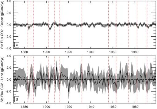
Statistically significant responses in both land and ocean fluxes of CO₂ are seen for

5

many, but not all, volcanic eruptions (Fig. 1c–d) – most noticeably for the larger erup-tions of Krakatau, Santa Maria, El Chichon, but not for Pinatubo.

While the physical response to volcanoes in the model is similar to observed, es-pecially for temperature, it is slightly weak in precipitation (Sect. 3.1), there was not a

significant response in atmospheric CO2 in the model (Fig. 2b). This could be due to

10

precipiation response, or due to the low climate feedback onto carbon in this model (Thornton et al., 2009), but represents a potential serious error in the model.

Jones and Cox (2001) used the Pinatubo eruption to analyze the sensitivity of the carbon cycle in a coupled-carbon-climate model, the HadCM3. Their model (Fig. 5,

blue bars) behaves differently in its climate, carbon cycle, and aerosol response than

15

the model used in this study (Thornton et al., 2009; Mahowald et al., 2011). While both models produce strong surface cooling in response to Pinatubo, the model here re-sponds more strongly with respect to reduced precipitation across much of the globe.

This difference is most prominent in the Amazon, where the model used by Jones and

Cox (2001) produces large increases in precipitation while our model sees a large de-20

crease (Fig. 5b). Observations suggest precipitation decreased in this region following Pinatubo (Trenberth and Dai, 2007), indicating that the model simulations presented here have a more accurate precipitation response than Jones and Cox (2001).

The model used by Jones and Cox (2001) also responds differently in terms of the

surface flux of CO2to the atmosphere; their model increases land uptake of CO2over

25

(14)

ESDD

3, 279–323, 2012

Title Page

Tables Figures

◭ ◮

Back Close

Full Screen / Esc

Discussion

P

a

per

|

Dis

cussion

P

a

per

|

Discussion

P

a

per

|

Discussio

n

P

a

per

|

analysis was repeated for shorter 1-yr and 2-yr time periods following the Pinatubo eruption, and while these shorter time periods had more significant and larger

anoma-lies (greater than±0.02 gC m−2day−1), the spatial variability did not change. The

“no-control” anomalies (Fig. 6b) tend to produce weaker uptake of CO2throughout a larger

part of the globe. 5

These changes in uptake of atmospheric CO2motivate an analysis of the modeled

carbon cycle and terrestrial biosphere. In the global average, there was a net global re-duction in gross and net primary prore-duction and heterotrophic respiration in the model following Pinatubo, but no significant response in net ecosystem production (Fig. 7a). The response in the Amazon (Fig. 7b) dominates the global response. In contrast, the 10

Jones and Cox (2001) simulations show significant terrestrial uptake of CO₂

associ-ated with increased net primary production and net ecosystem productivity, especially in the Amazon. In the global average, though, a decrease in heterotrophic respiration in their model contributes significantly to increases net ecosystem productivity.

The decreases in the modeled gross primary production are associated with anoma-15

lous decreases in both surface temperature and precipitation, and potentially increases

in diffuse radiation (Fig. 5b) in both the global average and in the Amazon. Decreases

in precipitation and surface temperature appear in the the observational record

fol-lowing Pinatubo (Hansen et al., 1996; Trenberth and Dai, 2007). A different response

occurs in the model used by Jones and Cox (2001); their model produces realistic sur-20

face cooling, but no significant response in precipitation. In particular, in the Amazon their model’s response to Pinatubo features possibly enhanced precipitation (Jones and Cox, 2001), which is not consistent with the data (Trenberth and Dai, 2007). A detailed analysis of the mechanisms for the response of land carbon to aerosols, and specifically volcanic aerosols, is important to understand the carbon cycle and aerosol 25

(15)

ESDD

3, 279–323, 2012

Title Page

Tables Figures

◭ ◮

Back Close

Full Screen / Esc

Discussion

P

a

per

|

Dis

cussion

P

a

per

|

Discussion

P

a

per

|

Discussio

n

P

a

per

|

Unfortunately, there are limited observations available to compare these modeled responses against. Grace et al. (1995) documented local and significant uptake of car-bon in the Amazon rainforest between 1992 and 1993, which is seen in the regional Amazon mean but not at a significant level (Fig. 7b), and in some limited regions of the Amazon where there is an uptake in carbon (Fig. 6). Tree ring records indicate 5

a decline in growth in Northern Hemisphere forests following Pinatubo (Krakauer and Randerson, 2003), and in temperate North America, while in the model simulations of North America there are some regions with an increase in uptake as well as some with a decrease. In addition to the results shown in Fig. 7, net primary production

de-creased in sub-Saharan Africa in the model following Pinatubo by−0.1±0.07 GtC yr−1.

10

By contrast, the signal over all the land in the tropics (30◦N–30◦S) was slightly stronger

and opposite in sign, 0.46±0.1 GtC yr−1. The growth rate of atmospheric CO2slowed

after the Pinatubo eruption, which is consistent with a net uptake of CO2 by the land

and oceans in the years after the eruption (Sarmiento et al., 2010), as seen in these simulations, although the signal was not statistically significant (Fig. 2b).

15

3.3 Average responses to volcanic eruptions

3.3.1 Globally averaged response

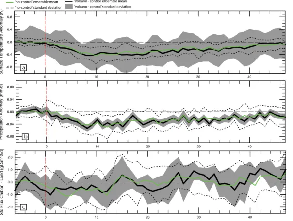
Similar to the modeled response to Pinatubo, in the average of the subset of 5 erup-tions from Table 1, surface temperatures and precipitation decrease following volcanic events (Fig. 8a–b). The same response is seen in the average of all the eruptions in 20

Table 1, but it is smaller in magnitude and more variable between eruptions. This is

partly because the selection of events spans eruptions which happened at different

latitudes and di_fferent times in the year.

Although there is a slight decrease in the flux of carbon into the land, there is not a statistically significant change in the modeled terrestrial or oceanic uptake of carbon fol-25

(16)

ESDD

3, 279–323, 2012

Title Page

Tables Figures

◭ ◮

Back Close

Full Screen / Esc

Discussion

P

a

per

|

Dis

cussion

P

a

per

|

Discussion

P

a

per

|

Discussio

n

P

a

per

|

the anomalies computed using the “no-control” method (Fig. 8e). This did not translate to significant signals in net primary production (Fig. 8f), although heterotrophic respi-ration decreased (Fig. 8g). A small increase in net ecosystem productivity (Fig. 8h) was seen in response to the eruptions, as was a small, but not statistically significant, increase in the flux of carbon to the atmosphere due to fires (Fig. 8i).

5

These averaged responses are somewhat damped compared to some of the individ-ual eruptions’ responses (not shown). This is partly due to the eruptions occurring at

dif-ferent times of the year; cooling or precipitation in di_fferent parts of the growing season

impact vegetation differently (Fig. 8c–h). Overall, a composite of the model’s response

to volcanoes suggest that gross primary production is reduced as is plant respiration, 10

which leaves net primary production slightly reduced but not statistically significantly. Because of the reduction in heterotrophic respiration, net ecosystem productivity is actually enhanced slightly, although much of the time this increase is not statistically significant. Note that most of these signals can be seen in both the “volcano-control” as well as the “no-control” anomalies.

15

3.3.2 Regional responses

Since the responses seen in Fig. 8 tended to be transient and last no more than two years, gridded average anomalies were computed for the first two year period following each eruption and averaged over the subset of 5 eruptions in Table 1 (Fig. 9).

The global signal in the carbon cycle’s response to volcanic eruptions is dominated 20

by responses in the tropics. Gross primary production is significantly reduced in the tropics regardless of the anomaly method chosen (Fig. 9a–b). Since gross primary production is a measure of photosynthesis at the ecosystem level, total growth and au-totrophic respiration in tropical ecosystems in the model is reduced following volcanic eruptions. Generally, the modeled net primary production is also decreased in these 25

regions (Fig. 9c–d), but not as much as gross primary production. The rate at which

plants return carbon during metabolism to the atmosphere as CO₂, autotrophic

(17)

ESDD

3, 279–323, 2012

Title Page

Tables Figures

◭ ◮

Back Close

Full Screen / Esc

Discussion

P

a

per

|

Dis

cussion

P

a

per

|

Discussion

P

a

per

|

Discussio

n

P

a

per

|

(NPP) (AR=GPP−NPP); since the modeled reductions in net primary production are

less than those in gross primary production, this implies that the modeled response to the eruptions here is a net increase in the amount of carbon returned to the atmosphere via plant metabolism.

However, a reduction in heterotrophic respiration (HR) (Fig. 9e–f) is also seen in 5

the modeled response to the eruptions; heterotrophic respiration measures the rate at which carbon is released to the atmosphere by the decomposition of organic matter in the soil, so a reduction in this component would reduce the amount of carbon being re-leased to the atmosphere. Ultimately, the net ecosystem productivity (NEP) throughout

much of the world increases in response to the eruptions (NEP=NPP−HR) (Fig. 9i–j),

10

albeit weakly outside of isolated regions in the Amazon and sub-Saharan Africa. Thus, in the modeled response to the eruptions, the terrestrial ecosystem becomes a net sink

of atmospheric CO2, which leads to a weak but significant uptake of carbon dioxide by

the terrestrial biosphere from the atmosphere (Fig. 9k–l; negative here denotes uptake of carbon, opposite the color scheme in Fig. 6). NPP went down, but HR went down 15

more, leaving more carbon on land.

There are not large discrepancies between the anomalies computed with the “volcano-control” method versus those computed with the “no-control” method in these results. In general, the “no-control” method yields more grid boxes with statistically significant anomalies, which tends to show up in the globally-averaged results as an 20

increase in the variance around the ensemble mean modeled response for a given variable.

Global and regional biological responses were computed for both the “volcano-control” and “no-“volcano-control” methods to compare the two techniques for estimating vol-canic anomalies. In the global average, the ‘volcano-control’ anomalies for the com-25

(18)

ESDD

3, 279–323, 2012

Title Page

Tables Figures

◭ ◮

Back Close

Full Screen / Esc

Discussion

P

a

per

|

Dis

cussion

P

a

per

|

Discussion

P

a

per

|

Discussio

n

P

a

per

|

in every variable for each region in Fig. 10. Nevertheless, the responses highlighted previously in Fig. 9 are corroborated by the regional responses in Fig. 10a–c. As sug-gested by Fig. 10c, the response in the mid- and high-latitudes in the Northern Hemi-sphere tended to be much weaker than the response in the tropics, which dominates the global total.

5

3.4 Ocean responses

The ocean biogeochemical response to volcanoes could be due to changes in temper-ature, winds, mixed layer depth, cloudiness and subsurface nutrient supply (Fig. 11), and here we neglect atmospheric deposition of nutrients. For nitrogen fixation, the Pa-cific tends to be iron limited, while the Atlantic tends to be phosphorous limited; thus 10

changes in nitrogen fixation, denitrification and net primary productivity (NPP) can have

multiple factors (Fig. 11b–c). O_ffthe west coast of North America, both net primary

pro-duction (Fig. 11a–b) and nitrogen fixation (Fig. 11c–d) show a shift, with increases in

both offthe coast and decreases surrounding, although the nitrogen fixation pattern

is slightly o_ffset from the NPP change. The increase in nitrogen fixation is associated

15

with a decrease in iron limitation due to an increase in dust deposition (Fig. 11g–h).

In the region where production increased, a decrease in outgassing of CO2 also

oc-curred (Fig. 11k–l). In the North Atlantic, there is also an increase associated with a

shift in nitrogen fixation. A time series analysis of the difference in productivity in the

volcano and control runs suggest that averaged over regions, volcanoes are not signfi-20

cant drivers of changes in productivity (Fig. 12); the response to di_fferent volcanoes can

be an increase or a decrease in productivity. A similar result is seen in the response of denitrification and nitrogen fixation of the ocean model to volcanoes (not shown). Overall, the oceanic biogeochemistry response to the eruptions is weaker than that on the land, although we ignore in these simulations the potentially important impact of 25

(19)

ESDD

3, 279–323, 2012

Title Page

Tables Figures

◭ ◮

Back Close

Full Screen / Esc

Discussion

P

a

per

|

Dis

cussion

P

a

per

|

Discussion

P

a

per

|

Discussio

n

P

a

per

|

focused on the ocean – including the effects of volcanic inputs on biogeochemical

species – will be completed.

4 Summary and discussion

An ensemble of model runs using the coupled-climate-carbon NCAR Community Cli-mate System Model Version 3 were integrated over the time period 1870–2000 to 5

investigate the response to volcanic eruptions. This study compares the CCSM3 re-sponse to volcanoes in the coupled-carbon-cycle framework to observations following Pinatubo, as well as extends previous studies (Jones and Cox, 2001) by looking at more eruptions.

In addition, we examine the ability to detect volcanoic signals in cases without a 10

control simulation. In the real world, there is no control case. Control cases represent expensive computation runs; thus deducing what part of the full response to volcanoes is possible to estimate from one simulation provides insight into model evaluation using volcanoes. The analysis here suggests that the globally averaged temperature and carbon dioxide response, as well as the regional scale response in temperature and 15

carbon dioxide fluxes are seen in the “no control” cases, even in the case shown here with a very weak response to the carbon cycle can be detected in the “no control” cases by volcanoes.

The model reproduces the expected reduction in globally averaged temperatures and globally averaged precipitation in a statistically significant manner for a short du-20

ration following the eruptions (Shindell et al., 2004; Trenberth and Dai, 2007). These dynamical responses are consistent with previous studies using this model (Schneider et al., 2009).

The model here produces surface cooling in response to the Pinatubo eruption sim-ilar in magnitude to the observed response. It also produces a statistically significant 25

(20)

ESDD

3, 279–323, 2012

Title Page

Tables Figures

◭ ◮

Back Close

Full Screen / Esc

Discussion

P

a

per

|

Dis

cussion

P

a

per

|

Discussion

P

a

per

|

Discussio

n

P

a

per

|

record, although precipitations responses are weaker than deduced from obsevations (Trenberth and Dai, 2007).

The physical climate response affects the response in the terrestrial biosphere. The

growth rate of atmospheric CO2 slowed after the Pinatubo eruption, which is

consis-tent with a net uptake of CO₂ by the land and oceans in the years after the

erup-5

tion (Sarmiento, 1993). These responses are broadly consistent with the model result. The carbon response in this model is weaker than seen in the observations or other model simulations (e.g., Jones et al., 2001). In another model, the HadCM3, there is a stronger net terrestrial uptake of carbon following the Pinatubo eruption primarily as-sociated with increases in gross primary production and net ecosystem productivity 10

especially in the Amazon (Jones et al., 2001). However, the HadCM3 model simulates an increase in precipitation, while observations and the model presented here show a decrease in precipitation in the Amazon, calling into question the robustness of their

result. The model here responds di_fferently, with significant decreases in gross primary

production and respiration, resulting in a weak response in net ecosystem productivity. 15

Furthermore, the model used by Jones et al. (2001) has strong coherence in its re-sponse, especially in South America and sub-Saharan Africa. The model here has far more spatial variability in its response than the Jones and Cox (2001) or Brovkin et al. (2010) studies in those same regions – particularly in South America.

It is not clear exactly why or where the model presented here is getting the CO₂

20

response wrong. There are not a large number of observations against which to com-pare the modeled volcanic response in the carbon cycle, but the model responds by

weakly increasing the uptake of CO₂from the atmosphere, particularly in South

Amer-ica. Grace et al. (1995) documented local, significant uptake of carbon in the Amazon rainforest between 1992 and 1993, while Krakauer and Randerson (2003) noted that 25

(21)

ESDD

3, 279–323, 2012

Title Page

Tables Figures

◭ ◮

Back Close

Full Screen / Esc

Discussion

P

a

per

|

Dis

cussion

P

a

per

|

Discussion

P

a

per

|

Discussio

n

P

a

per

|

consistent with the low climate impact on the carbon cycle seen previously (Thornton et al., 2009), and suggests that volcanoes do provide insight into the climate-carbon feedback, as previously argued (Jones et al., 2001; Friedlingstein and Prentice, 2010). More data and approaches are needed in order to constrain the volcanic response; for example, the use of carbon isotopes (Welp et al., 2011) to better estimate biosphere-5

atmosphere exchanges.

In the composite of the set of eruptions analyzed in this study, a similar story emerges to that seen when just analyzing Pinatubo. Again, in the global average, there is a signif-icant reduction in both respiration and gross primary production in the mean response to volcanic eruptions, as well as a small but non-significant increase in net ecosys-10

tem productivity, indicating a small uptake of carbon by the terrestrial biosphere from the atmosphere after the eruptions. This response is most prominent when averaged over the first two years following the eruptions, and is consistent throughout the tropics. This average response is also consistent with the modeled response to Pinatubo but slightly larger when averaged over many eruptions. The carbon response of the ocean 15

is smaller than that of the land in these simulations, similar to previous studies (Jones and Cox, 2001; Brovkin et al., 2010); however, these studies ignore the potentially

im-portant effects of the addition of biogeochemically relevant species in the volcanic ash

(e.g., Watson, 1997).

Acknowledgements. This work was done under the auspices of NASA NNGO6G127G and

20

(22)

ESDD

3, 279–323, 2012

Title Page

Tables Figures

◭ ◮

Back Close

Full Screen / Esc

Discussion

P

a

per

|

Dis

cussion

P

a

per

|

Discussion

P

a

per

|

Discussio

n

P

a

per

|

References

Adams, J. B., Mann, M. E., and Ammann, C. M.: Proxy evidence for an El Nino-like response to volcanic forcing, Nature, 426, 274–278, doi:10.1038/nature02101, 2003. 281, 282 Ammann, C. M., Meehl, G. A., Washington, W. M., and Zender, C. S.: A monthly and latitudinally

varying volcanic forcing dataset in simulations of 20th century climate, Geophys. Res. Lett.,

5

30, 1657–1671, doi:10.1029/2003GL016875, 2003. 284, 285

Bousquet, P., Peylin, P., Ciais, P., Le Qu ´er ´e, C., Friedlingstein, P., and Tans, P. P.: Regional Changes in Carbon Dioxide Fluxes of Land and Oceans Since 1980, Science, 290, 1342– 1346, doi:10.1126/science.290.5495.1342, 2000. 283

Brovkin, V., Lorenz, S. J., Jungclaus, J., Raddatz, T., Timmreck, C., Reick, C. H., Segschneider,

10

J., and Six, K.: Sensitivity of a coupled climate-carbon cycle model to large volcanic eruptions during the last millennium, Tellus B, 62, 674–681, doi:10.1111/j.1600-0889.2010.00471.x, 2010. 283, 298, 299

Collins, W. D., Bitz, C. M., Blackmon, M. L., Bonan, G. B., Bretherton, C. S., Carton, J. A., Chang, P., Doney, S. C., Hack, J. J., Henderson, T. B., Kiehl, J. T., Large, W. G., McKenna,

15

D. S., Santer, B. D., and Smith, R. D.: The Community Climate System Model Version 3 (CCSM3), J. Climate, 19, 2122–2143, doi:10.1175/JCLI3761.1, 2006a. 284

Collins, W. D., Rasch, P. J., Boville, B. A., Hack, J. J., McCaa, J. R., Williamson, D. L., Briegleb, B. P., Bitz, C. M., Lin, S.-J., and Zhang, M.: The Formulation and Atmospheric Simula-tion of the Community Atmosphere Model Version 3 (CAM3), J. Climate, 19, 2144–2161,

20

doi:10.1175/JCLI3760.1, 2006b. 284, 289

Cox, P. M., Betts, R. A., Jones, C. D., Spall, S. A., and Totterdell, I. J.: Acceleration of global warming due to carbon-cycle feedbacks in a coupled climate model, Nature, 408, 184–187, doi:10.1038/35041539, 2000. 283

Deser, C., Capotondi, A., Saravanan, R., and Phillips, A. S.: Tropical Pacific and Atlantic Climate

25

Variability in CCSM3, J. Climate, 19, 2451–2481, doi:10.1175/JCLI3759.1, 2006. 284 Doney, S. C., Lima, I., Feely, R. A., Glover, D. M., Lindsay, K., Mahowald, N., Moore, J. K.,

and Wanninkhof, R.: Mechanisms governing interannual variability in upper-ocean inorganic carbon system and air-sea CO₂ fluxes: Physical climate and atmospheric dust, Deep-Sea Res. Pt. II, 56, 640–655, doi:10.1016/j.dsr2.2008.12.006, 2009a. 285

(23)

ESDD

3, 279–323, 2012

Title Page

Tables Figures

◭ ◮

Back Close

Full Screen / Esc

Discussion

P

a

per

|

Dis

cussion

P

a

per

|

Discussion

P

a

per

|

Discussio

n

P

a

per

|

Doney, S. C., Lima, I., Moore, J. K., Lindsay, K., Behrenfeld, M. J., Westberry, T. K., Ma-howald, N., Glover, D. M., and Takahashi, T.: Skill metrics for confronting global upper ocean ecosystem-biogeochemistry models against field and remote sensing data, skill assess-ment for coupled biological/physical models of marine systems, J. Mar. Syst., 76, 95–112, doi:10.1016/j.jmarsys.2008.05.015, 2009b. 285

5

Duggen, S., Croot, P., Schacht, U., and Hoffmann, L.: Subduction zone volcanic ash can fertilize the surface ocean and stimulate phytoplankton growth: Evidence from biogeochemical ex-periments and satellite data, Geophys. Res. Lett., 34, L01612, doi:10.1029/2006GL027522, 2007. 283

Duggen, S., Olgun, N., Croot, P., Hoffmann, L., Dietze, H., Delmelle, P., and Teschner, C.:

10

The role of airborne volcanic ash for the surface ocean biogeochemical iron-cycle: a review, Biogeosciences, 7, 827–844, doi:10.5194/bg-7-827-2010, 2010. 283

Emile-Geay, J., Seager, R., Cane, M. A., Cook, E. R., and Haug, G. H.: Volcanoes and ENSO over the Past Millennium, J. Climate, 21, 3134–3148, 2008. 281

Friedlingstein, P. and Prentice, I.: Carbon–climate feedbacks: a review of model

15

and observation based estimates, Curr. Opin. Environ. Sustain., 2, 251–257, doi:10.1016/j.cosust.2010.06.002, 2010. 283, 299

Friedlingstein, P., Cox, P., Betts, R., Bopp, L., von Bloh, W., Brovkin, V., Cadule, P., Doney, S., Eby, M., Fung, I., Bala, G., John, J., Jones, C., Joos, F., Kato, T., Kawamiya, M., Knorr, W., Lindsay, K., Matthews, H. D., Raddatz, T., Rayner, P., Reick, C., Roeckner, E., Schnitzler,

K.-20

G., Schnur, R., Strassmann, K., Weaver, A. J., Yoshikawa, C., and Zeng, N.: Climate-Carbon Cycle Feedback Analysis: Results from the C4MIP Model Intercomparison, J. Climate, 19, 3337–3353, doi:10.1175/JCLI3800.1, 2006. 283

Frogner, P., G ´oslason, S. R., and Oskarsson,´ N.: Fertilizing potential of vol-canic ash in ocean surface water, Geology, 29, 487–490,

doi:10.1130/0091-25

7613(2001)029<_0487:FPOVAI>_{2.0.CO;2, 2001. 283}

Grace, J., Lloyd, J., McIntyre, J., Miranda, A. C., Meir, P., Miranda, H. S., Nobre, C., Moncrieff, J., Massheder, J., Malhi, Y., Wright, I., and Gash, J.: Carbon Dioxide Uptake by an Undis-turbed Tropical Rain Forest in Southwest Amazonia, 1992 to 1993, Science, 270, 778–780, doi:10.1126/science.270.5237.778, 1995. 293, 298

(24)

ESDD

3, 279–323, 2012

Title Page

Tables Figures

◭ ◮

Back Close

Full Screen / Esc

Discussion

P

a

per

|

Dis

cussion

P

a

per

|

Discussion

P

a

per

|

Discussio

n

P

a

per

|

Hansen, J., Sato, M., Ruedy, R., Lacis, A., Asamoah, K., Borenstein, S., Brown, E., Cairns, B., Caliri, G., and Campbell, M.: A Pinatubo Climate Modeling Investigation, in: The Mount Pinatubo Eruption: Effects on the Atmosphere and Climate, edited by: Fiocco, G., Fua, D., and Visconti, G., vol. 1, Springer-Verlag, Berlin, Heidelberg, 233–272, 1996. 282, 292 Jones, C. D. and Cox, P. M.: Modeling the volcanic signal in the atmospheric CO₂record, Global

5

Biogeochem. Cy., 15, 453–465, doi:10.1029/2000GB001281, 2001. 283, 284, 286, 291, 292, 297, 298, 299, 308, 313

Jones, C. D., Collins, M., Cox, P. M., and Spall, S. A.: The Carbon Cycle Response to ENSO: A Coupled Climate Carbon Cycle Model Study, J. Climate, 14, 4113–4129, doi:10.1175/1520-0442(2001)014<_4113:TCCRTE>_{2.0.CO;2, 2001. 282, 288, 298, 299}

10

Jones, P. D. and Kelly, P. M.: The Effect of Tropical Explosive Volcanic Eruptions on Surface Air Temperature, in: The Mount Pinatubo Eruption: Effects on the Atmosphere and Climate, edited by: Fiocco, G., Fua, D., and Visconti, G., Springer-Verlag, Berlin, Heidelberg, 95–111, 1996. 308

Krakauer, N. Y. and Randerson, J. T.: Do volcanic eruptions enhance or diminish net

pri-15

mary production? Evidence from tree rings, Global Biogeochem. Cy., 17, 1118–1129, doi:10.1029/2003GB002076, 2003. 282, 293, 298

Le Qu ´er ´e, C., Raupach, M. R., Canadell, J. G., and Marland, G.: Trends in the sources and sinks of carbon dioxide, Nat. Geosci., 2, 831–836, doi:10.1038/ngeo689, 2009. 283

Mahowald, N., Lindsay, K., Rothenberg, D., Doney, S. C., Moore, J. K., Thornton, P.,

Rander-20

son, J. T., and Jones, C. D.: Desert dust and anthropogenic aerosol interactions in the Com-munity Climate System Model coupled-carbon-climate model, Biogeosciences, 8, 387–414, doi:10.5194/bg-8-387-2011, 2011. 283, 284, 285, 286, 291

Mahowald, N. M., Muhs, D. R., Levis, S., Rasch, P. J., Yoshioka, M., Zender, C. S., and Luo, C.: Change in atmospheric mineral aerosols in response to climate: Last glacial period,

prein-25

dustrial, modern, and doubled carbon dioxide climates, J. Geophys. Res., 111, D10202, doi:10.1029/2005JD006653, 2006. 285

Mass, C. F. and Portman, D. A.: Major Volcanic Eruptions and Climate: A Critical Evaluation, J. Climate, 2, 566–593, 1989. 281

Meehl, G. A., Washington, W. M., Santer, B. D., Collins, W. D., Arblaster, J. M., Hu, A., Lawrence,

30

(25)

ESDD

3, 279–323, 2012

Title Page

Tables Figures

◭ ◮

Back Close

Full Screen / Esc

Discussion

P

a

per

|

Dis

cussion

P

a

per

|

Discussion

P

a

per

|

Discussio

n

P

a

per

|

Moore, J. K., Doney, S. C., and Lindsay, K.: Upper ocean ecosystem dynamics and iron cycling in a global three-dimensional model, Global Biogeochem. Cy., 18, GB4028, doi:10.1029/2004GB002220, 2004. 285

Nemani, R. R., Keeling, C. D., Hashimoto, H., Jolly, W. M., Piper, S. C., Tucker, C. J., Myneni, R. B., and Running, S. W.: Climate-Driven Increases in Global Terrestrial Net Primary

Pro-5

duction from 1982 to 1999, Science, 300, 1560–1563, doi:10.1126/science.1082750, 2003. 282

Oman, L., Robock, A., Stenchikov, G., Schmidt, G. A., and Ruedy, R.: Climatic response to high-latitude volcanic eruptions, J. Geophys. Res., 110, D13103, doi:10.1029/2004JD005487, 2005. 281, 286

10

Randerson, J. T., Hoffman, F. M., Thornton, P. E., Mahowald, N. M., Lindsay, K., Lee, Y.-H., Nevi-son, C. D., Doney, S. C., Bonan, G., St ¨ockli, R., Covey, C., Running, S. W., and Fung, I. Y.: Systematic Assessment of Terrestrial Biogeochemistry in Coupled Climate-Carbon Models, Global Change Biol., 15, 2462–2484, doi:10.1111/j.1365-2486.2009.01912.x, 2009. 285 Robock, A. and Liu, Y.: The Volcanic Signal in Goddard Institute for Space

Stud-15

ies Three-Dimensional Model Simulations, J. Climate, 7, 44–55, doi:10.1175/1520-0442(1994)007<0044:TVSIGI>2.0.CO;2, 1994. 286

Robock, A. and Mao, J.: Winter warming from large volcanic eruptions, Geophys. Res. Lett., 19, 2405–2408, doi:10.1029/92GL02627, 1992. 281, 286, 305

Robock, A. and Mao, J.: The Volcanic Signal in Surface Temperature Observations, J. Climate,

20

8, 1086–1103, 1995. 281, 289

Sarmiento, J. L.: Atmospheric CO₂ stalled, Nature, 365, 697–698, doi:10.1038/365697a0, 1993. 282, 290, 298

Sarmiento, J. L., Gloor, M., Gruber, N., Beaulieu, C., Jacobson, A. R., MikaloffFletcher, S. E., Pacala, S., and Rodgers, K.: Trends and regional distributions of land and ocean carbon

25

sinks, Biogeosciences, 7, 2351–2367, doi:10.5194/bg-7-2351-2010, 2010. 283, 293

Schneider, D. P., Ammann, C. M., Otto-Bliesner, B. L., and Kaufman, D. S.: Climate response to large, high-latitude and low-latitude volcanic eruptions in the Community Climate System Model, J. Geophys. Res., 114, D15101, doi:10.1029/2008JD011222, 2009. 284, 286, 289, 297

30

(26)

ESDD

3, 279–323, 2012

Title Page

Tables Figures

◭ ◮

Back Close

Full Screen / Esc

Discussion

P

a

per

|

Dis

cussion

P

a

per

|

Discussion

P

a

per

|

Discussio

n

P

a

per

|

Sitch, S., Huntingford, C., Gedney, N., Levy, P. E., Lomas, M., Piao, S. L., Betts, R., Ciais, P., Cox, P., Friedlingstein, P., Jones, C. D., Prentice, I. C., and Woodward, F. I.: Evaluation of the terrestrial carbon cycle, future plant geography and climate-carbon cycle feedbacks using five Dynamic Global Vegetation Models (DGVMs), Global Change Biol., 14, 2015– 2039, doi:10.1111/j.1365-2486.2008.01626.x, 2008. 283

5

Stenchikov, G., Hamilton, K., Stouffer, R. J., Robock, A., Ramaswamy, V., Santer, B., and Graf, H.-F.: Arctic Oscillation response to volcanic eruptions in the IPCC AR4 climate models, J. Geophys. Res., 111, D07107, doi:10.1029/2005JD006286, 2006. 281, 286, 289

Thornton, P. E., Lamarque, J.-F., Rosenbloom, N. A., and Mahowald, N. M.: Influence of carbon-nitrogen cycle coupling on land model response to CO₂ fertilization and climate variability,

10

Global Biogeochem. Cy., 21, GB4018, doi:10.1029/2006GB002868, 2007. 285

Thornton, P. E., Doney, S. C., Lindsay, K., Moore, J. K., Mahowald, N., Randerson, J. T., Fung, I., Lamarque, J.-F., Feddema, J. J., and Lee, Y.-H.: Carbon-nitrogen interactions reg-ulate climate-carbon cycle feedbacks: results from an atmosphere-ocean general circulation model, Biogeosciences, 6, 2099–2120, doi:10.5194/bg-6-2099-2009, 2009. 283, 284, 285,

15

291, 299

Trenberth, K. E. and Dai, A.: Effects of Mount Pinatubo volcanic eruption on the hy-drological cycle as an analog of geoengineering, Geophys. Res. Lett., 34, L15702, doi:10.1029/2007GL030524, 2007. 282, 289, 290, 291, 292, 297, 298

Watson, A. J.: Volcanic iron, CO₂, ocean productivity and climate, Nature, 385, 587–588,

20

doi:10.1038/385587b0, 1997. 283, 299

Welp, L. R., Keeling, R. F., Meijer, H. A. J., Bollenbacher, A. F., Piper, S. C., Yoshimura, K., Francey, R. J., Allison, C. E., and Wahlen, M.: Interannual variability in the oxygen isotopes of atmospheric CO₂driven by El Nino, Nature, 477, 579–582, doi:10.1038/nature10421, 2011. 299

25

Yeager, S. G., Shields, C. A., Large, W. G., and Hack, J. J.: The Low-Resolution CCSM3, J. Climate, 19, 2545–2566, doi:10.1175/JCLI3744.1, 2006. 284

Zender, C. S., Bian, H., and Newman, D.: Mineral Dust Entrainment and Deposition (DEAD) model: Description and 1990s dust climatology, J. Geophys. Res., 108, 4416, doi:10.1029/2002JD002775, 2003. 285

(27)

ESDD

3, 279–323, 2012

Title Page

Tables Figures

◭ ◮

Back Close

Full Screen / Esc

Discussion

P

a

per

|

Dis

cussion

P

a

per

|

Discussion

P

a

per

|

Discussio

n

P

a

per

|

Table 1.Years of selected volcanic eruptions modified from Robock and Mao (1992).

Volcano Eruption Year Lat. DVI2 VEI3

Krakatau1 1883 6◦S 1000 6

Tarawera 1886 38◦S 800 5

Bandai 1888 38◦N 500 4

Santa Maria1 1902 15◦S 600 6

Ksudach 1907 52◦N 500 5

Katmai 1912 58◦N 500 6

Quizapu 1932 36◦S 70 5

Bezymianny 1956 56◦N 30 5

Agung1 1963 8◦S 800 4

Fuego 1974 14◦N 250 4

El Chich ´on1 1982 17◦N 800 5 Mt. Pinatubo1 1991 15◦

N 1000 6

(28)

ESDD

3, 279–323, 2012

Title Page

Tables Figures

◭ ◮

Back Close

Full Screen / Esc

Discussion

P

a

per

|

Dis

cussion

P

a

per

|

Discussion

P

a

per

|

Discussio

n

P

a

per

|

(29)

ESDD

3, 279–323, 2012

Title Page

Tables Figures

◭ ◮

Back Close

Full Screen / Esc

Discussion

P

a

per

|

Dis

cussion

P

a

per

|

Discussion

P

a

per

|

Discussio

n

P

a

per

|