www.the-cryosphere.net/10/3063/2016/ doi:10.5194/tc-10-3063-2016
© Author(s) 2016. CC Attribution 3.0 License.
Critical investigation of calculation methods for the
elastic velocities in anisotropic ice polycrystals
Agnès Maurel1, Jean-François Mercier2, and Maurine Montagnat3 1Institut Langevin, CNRS, ESPCI ParisTech, 1 rue Jussieu, 75005 Paris, France
2Poems, CNRS, ENSTA ParisTech, INRIA, 828 boulevard des Maréchaux, 91762 Palaiseau, France 3LGGE, CNRS, Université Grenoble Alpes, 38041 Grenoble, France.
Correspondence to:Agnès Maurel ([email protected])
Received: 25 January 2016 – Published in The Cryosphere Discuss.: 9 February 2016 Revised: 20 May 2016 – Accepted: 9 June 2016 – Published: 16 December 2016
Abstract.Crystallographic texture (or fabric) evolution with depth along ice cores can be evaluated using borehole sonic logging measurements. These measurements provide the ve-locities of elastic waves that depend on the ice polycrystal anisotropy, and they can further be related to the ice tex-ture. To do so, elastic velocities need to be inverted from a modeling approach that relate elastic velocities to ice texture. So far, two different approaches can be found. A classical model is based on the effective medium theory; the veloc-ities are derived from elastic wave propagation in a homo-geneous medium characterized by an average elasticity ten-sor. Alternatively, a velocity averaging approach was used in the glaciology community that averages the velocities from a given population of single crystals with different orienta-tions.
In this paper, we show that the velocity averaging method is erroneous in the present context. This is demonstrated for the case of waves propagating along the clustering direction of a highly textured polycrystal, characterized by crystallo-graphic caxes oriented along a single maximum (cluster). In this case, two different shear wave velocities are obtained while a unique velocity is theoretically expected. While mak-ing use of this velocity averagmak-ing method, reference work by Bennett (1968) does not end with such an unphysical result. We show that this is due to the use of erroneous expressions for the shear wave velocities in a single crystal, as the starting point of the averaging process.
Because of the weak elastic anisotropy of ice single crys-tal, the inversion of the measured velocities requires accurate modeling approaches. We demonstrate here that the
inver-sion method based on the effective medium theory provides physically based results and should therefore be favored.
1 Introduction
Wave propagation in glaciology is mostly regarded in the context of seismic waves; see, e.g., Kohnen (1974) and Blankenship et al. (1987). More recently, a new interest has emerged with the idea of using in situ wave velocity mea-surements along ice boreholes in order to evaluate the tex-ture (fabric) anisotropy and its evolution with depth along deep ice cores. Such measurements are based on sonic log-ging that evaluates the travel time of elastic waves propagat-ing in the ice over a short distance (typically few meters). A classical sonic logger was recently used during a measure-ment campaign at EPICA Dome C (East Antarctica) (Gus-meroli et al., 2012) and revealed the sensitivity of the elas-tic velocities on the degree of anisotropy of ice polycrystals characterized by a cluster-type texture (withcaxis orienta-tions clustered around the vertical direction) that varies with depth. The measured velocity changes are small, and the in-version procedure to access the texture estimation is depen-dent on the level of uncertainties in the measurements. Strong motivation therefore arises for the development of accurate modeling for the inversion of the elastic velocities into the local ice anisotropy.
trans-verse isotropy (VTI), as described before, and girdles with a horizontal transverse isotropy (HTI). The latter corresponds to crystallographiccaxes mostly aligned in a vertical plan, which form in situations where a horizontal tension domi-nates the stress field. The model used relies on the definition of an “effective medium” characterized by an averaged elas-ticity tensor defined at the scale of many grains (the polycrys-tal). Maurel et al. (2015) presented a comparison with Ben-nett’s predictions (Bennett, 1968), which are based on the ve-locity averaging method, and illustrated the weak differences in the velocities predicted by the two models for VTI clus-tered textures. Contrary to the effective medium theory, the velocity averaging method does not rely on a rigorous math-ematical formalism. Thus, beyond the relative agreement ob-served for clustered textures, the correctness of the velocity averaging method can be questioned.
This is the goal of the present paper. We will show that the velocity averaging method is based on an erroneous fun-damental assumption. To do so, we perform a demonstration for the cases of cluster and girdle ice textures with VTI. It is found that a wave propagating along the vertical axis is associated with two different shear velocities, which is un-physical since the polarizations of the shear waves are in the plane of isotropy. In Bennett (1968) a unique expression of the shear velocity was obtained, starting with modified ex-pressions of the two shear wave velocities in ice single crys-tals. The modification consisted in attributing symmetrical weights to both velocities in order to get the same value after the velocity averaging. It resulted in a velocity value close to the harmonic mean of the two unphysical shear velocities derived from the direct use of the velocity averaging method. Considering the low elastic anisotropy of the ice single crystal, the accuracy of the inversion procedure from the measured velocities to ice texture is essential. In particular, a model relying on a rigorous mathematical formalism is re-quired, in order to describe the case of complex textures, be-yond the simple case of VTI clusters. With regard to this re-quirement, we will show that the model based on the effective medium theory appears more reliable.
2 Classical results on polycrystal effective anisotropy and wave propagation in anisotropic media
In this section, we recall classical results (i) on the propaga-tion of elastic waves in a crystal or in a polycrystal charac-terized by a uniform elasticity tensor and (ii) on the elasticity tensor of polycrystals, considered at the scale of many grains as an equivalent “single” crystal. This allows us to introduce the notations that will be used further in the text and to clarify in a self-consistent way some properties that will be needed.
2.1 Wave propagation in a uniform anisotropic medium – the Christoffel equation
In the following, we denotex =(x1,x2,x3) the spatial co-ordinates,u(x)=(u1(x),u2(x),u3(x)) the elastic displace-ment vector,ρthe constant mass density andcabcdthe elas-ticity tensor being uniform in space. The case of a uniform
cabcdcorresponds either to a single crystal or to a polycrystal thought as an effective medium; in this latter case,cabcd char-acterizes the texture of the polycrystal. The propagation of monochromatic waves of frequencyω is described by the wave equation
ρω2ua(x)+cabcd
∂2 ∂xb∂xc
ud(x)=0, (1)
witha=1, 2, 3 and where repeated indices mean summation (Einstein convention). Denotingk=knthe wave vector (kis the wave number) with n=(n1,n2, n3) the unitary vector alongk, the elastic displacement readsua(x)=Uaeik·x lead-ing toρω2Ua−k2cabcdnbncUd=0 fora=1, 2, 3. This sys-tem of equations admits nonzero solutions for (U1, U2, U3) if the determinant of the matrixρω2δad−k2cabcdnbnc van-ishes (δab is the Kronecker symbol). One gets the disper-sion relation that links k and ω; equivalently, introducing the phase velocityV =ω/ k, we get the classical form of the Christoffel equation
DethρV2δad−cabcdnbnc i
=0. (2)
The Christoffel equation admits in general three solutions,
V=VP,VSH, VSV, that are the elastic velocities of the lon-gitudinal wave and the two transverse waves (P, SH and SV stand for pressure wave, shear horizontal and shear ver-tical waves). It is important to stress at this point that be-cause the three values ofV2are the eigenvalues of the matrix
cabcdnbnc/ρ, they do not depend on the particular frame (e1, e2,e3) used to expresscabcd. On the contrary, the eigenvec-tors (U1,U2,U3) associated with the eigenvalues obviously depend on the frame where they are expressed.
2.2 Elasticity tensor of the polycrystal resulting from anisotropy from grain to grain
In the previous section, we have considered the uniform elas-ticity tensor of a polycrystal. This elaselas-ticity tensor is de-rived from the characteristics of the grains which compose the polycrystal. For ice, each grain is composed of the same single crystal, with hexagonal symmetry being characterized by its elasticity tensorc0ij kl, written in terms of CI J0 in the Voigt’s notation (Voigt, 1928). The superscript 0 refers to an elasticity tensor expressed in the frame of its principal axes, with thecaxis being oriented alonge3, hereafter referred as the vertical axis. The Voigt’s matrixC0(with elementsC0
I J,
C0=
A A−2N F 0 0 0
A−2N A F 0 0 0
F F C 0 0 0
0 0 0 L 0 0
0 0 0 0 L 0
0 0 0 0 0 N
, (3)
with the standard notations
cij kℓ→CI J,
for(i, j )→I, (k, l)→J,
and(1,1)→1, (2,2)→2, (3,3)→3,
(3,2), (2,3)→4, (3,1), (1,3)→5, (1,2), (2,1)→6
. (4)
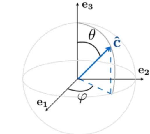
For an arbitrary direction of thecaxis (Fig. 1)
ˆ
c=(sinθcosϕ,sinθsinϕ,cosθ ), (5) the elasticity tensorcabcdis deduced fromc0ij klfollowing
cabcd=RiaRj bRkcRldcij kℓ0 , (6) withRthe rotation matrix (with elementsRij):
R≡
cosθcosϕ cosθsinϕ −sinθ
−sinϕ cosϕ 0
sinθcosϕ sinθsinϕ cosθ
. (7)
cabcddepends on (θ,ϕ), which are the usual angles in spher-ical coordinates.
The anisotropy at the macroscopic scale (at the scale of many grains) results from the many (or few) possible orien-tations of thecaxis in each grain. This distribution ofcaxes is defined by a probability distribution functionp(θ,ϕ) sat-isfying
Z
dp(θ, ϕ)=1,with d=sinθdθdϕ. (8)
The elasticity tensor ceffij kl and the associated Voigt’s ma-trix CeffI J of the polycrystal can be calculated by means of the average of the elasticity tensors of the grains following
ceffij kl= Z
dp(ϕ, θ )cij kl,CeffI J= Z
dp(ϕ, θ )CI J, (9) with the same index convention, Eq. (4), between the elastic-ity tensorceffij kl and the Voigt matrixCeffI J. For VTI textures, the direction of the axis of anisotropy is given by the effective
caxis, denotedcˆeff.
For the numerical application, we will use the elastic con-stants as used in Bennett (1968):
Ice single crystal
A =14.06×10⁹N m−2, C=15.24×10⁹N m−2, L=3.06×10⁹N m−2,
N =3.455×10⁹N m−2, F=5.88×10⁹N m−2, ρ=917kg m−3
. (10)
Figure 1.Spherical angles (ϕ,θ) used for the orientation of the caxis, (cˆis an unitary vector).
3 Elastic wave velocities in the velocity averaging method and velocities of the effective medium for VTI textures
In this section, we compare the elastic velocities obtained from the velocity averaging method, as used in Bennett (1968), Gusmeroli et al. (2012) and Vélez et al. (2016), and the elastic velocities obtained from the effective medium the-ory. The two approaches are as follows.
1. Velocities from the velocity averaging method: first, solve the Christoffel equation for given (θ,ϕ) using
V (θ, ϕ)=VP, VSV, VSHare the roots of DethρV2δil−cij klnjnk
i .
Then compute the average of the slowness, from which
Vav= Z
dp(θ, ϕ)V−1(θ, ϕ) −1
. (11)
2. Velocities of the effective medium: first, compute the effective elasticity tensor using
ceffij kl= Z
dp(θ, ϕ)cij kl.
Then, solve the Christoffel equation:
V =VPeff, VSVeff, VSHeffare the roots of DethρV2δil−cij kleff njnk
i
. (12)
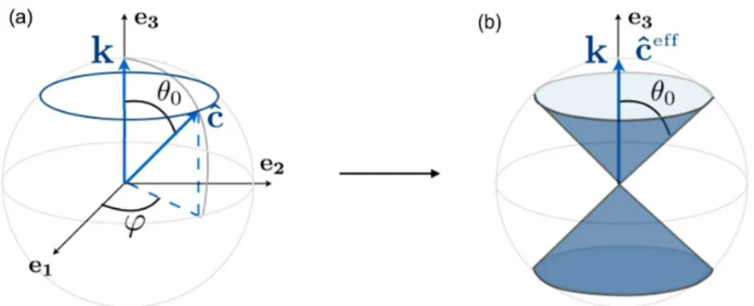
Figure 2.First configuration of a VTI girdle with a single zenith angleθ0.(a)shows a typicalcaxiscˆ=(sinθ0cosϕ, sinθ0sinϕ, cosθ0) within one grain, with a constantθ0, andϕvaries randomly from grain to grain.(b)shows the resulting VTI texture of the polycrystal at the macroscopic scale.cˆeffis the effectivecaxis.
Figure 3.Second configuration of the usual VTI clustered texture.(a)shows a typicalcaxiscˆ=(sinθcosϕ, sinθsinϕ, cosθ) within one grain, whereθvaries in [0,θ0] andϕvaries randomly from grain to grain.(b)shows the resulting clustered, VTI, texture of the polycrystal at the macroscopic scale.cˆeffis the effectivecaxis.
Two examples of VTI structures will be presented and the propagation along the vertical direction is considered. The first structure is artificial, with acaxis associated with a unique θ=θ0 value in [0,π/2] (andϕ∈[0, 2π]), but it provides explicit expressions of the velocities in both ap-proaches. It could be seen as a girdle with VTI (Azuma and Goto-Azuma, 1996) with a single zenith angle θ0 (Fig. 2). The second example corresponds to a cone representative of clustered textures measured along ice cores (Gusmeroli et al., 2012; Diez and Eisen, 2015), with θ∈[0, θ0] (and ϕ∈[0, 2π]), and is studied numerically (Fig. 3).
3.1 Wave propagation along the vertical axis in a polycrystal with VTI
We consider a wave propagating along the vertical axis, thus k=(0, 0,k), in a polycrystal with VTI (Figs. 2 and 3). The VTI structure provides thatϕ∈[0, 2π] and is associated with a probability distribution independent ofϕ. Thus, the distri-bution ofcaxes is given by probability distribution functions of the form
p(θ, ϕ)=Pθ0(θ )
2π ,with
π/2 Z
0
dθsinθ Pθ0(θ )=1. (13)
3.1.1 Velocities from the velocity averaging method In this method, we first derive the velocities in a grain, and this is done without lack of generality for a wave propagat-ing alonge3. The Christoffel equation, Eq. (2) withnb=δb3 (same fornc), simplifies to
ρV2−C55 −C45 −C35
−C45 ρV2−C44 −C34
−C35 −C34 ρV2−C33
=0, (14)
C33 =Asθ4+2(2L+F )sθ2cθ2+Ccθ4
C44 =(A+C−2F )sθ2cθ2sϕ2+L
sϕ2cθ2−sθ22
+cθ2cϕ2i+N sθ2cϕ2 C55 =(A+C−2F )sθ2cθ2cϕ2+L
cϕ2cθ2−sθ22
+cθ2sϕ2i+N sθ2sϕ2 C34 = −sϕsθ cθ
h
Asθ2−Ccθ2+(2L+F )1−2sθ2i C35 = −cϕsθ cθ
h
Asθ2−Ccθ2+(2L+F )1−2sθ2i C45 =sϕcϕsθ2
h
(A+C−2F )cθ2+L1−4cθ2−Ni
(15)
We have used the notationscϕ≡cosϕ,sϕ≡sinϕ,sθ≡sinθ
andcθ≡cosθ. The determinant, Eq. (14), can be calculated and we get the rootsρV2:
ρV2 = Lcθ2+N sθ2 ,
ρV22 + Asθ2+Ccθ2+LρV2−F2sθ2cθ2 +ACsθ2cθ2+ALsθ4+CLcθ4 −2F Lsθ2cθ2=0
. (16)
The first root corresponds to a pure shear wave polarized in a direction perpendicular to bothkandcˆ, referred as the SH wave. The two roots of the second equation are associated with the so-called quasi-shear and quasi-longitudinal waves, being coupled. The directions of polarization of the three waves are orthogonal (because the determinant is associated with a symmetric matrix) but the quasi-longitudinal wave is in general not alonge3and the quasi-shear wave is in general not in the (e1,e2) plane. More explicitly, the three velocities read
ρVSH2 =Lcθ2+N sθ2, ρVSV2 =1
2 h
C+L+(A−C)sθ2−√D i
,
ρVP2=1
2 h
C+L+(A−C)sθ2+√Di,
(17)
with
D≡
h
Asθ2−Ccθ2 i h
Asθ2−Ccθ2+2L
cθ2−sθ2 i
+4sθ2cθ2
F2+2F L
+L2.
These are the expressions of the velocities in a single grain with acaxis forming an angleθwithk.
The second step in the velocity averaging method can be applied:
1
Vav(θ 0)=
2π Z 0 dϕ π/2 Z 0
dθsinθp(θ, ϕ)V−1(θ, ϕ)
=
π/2 Z
0
dθsinθ Pθ0(θ )V−
1(θ ), (18)
for V=VSH,VSV,VPtaken from Eq. (17). These last aver-ages depend further onPθ0(θ ).
3.1.2 Velocities of the effective medium
With the probability function given by Eq. (13), the effective medium is characterized by a Voigt matrix:
CeffI J(θ0)= 2π Z 0 dϕ 2π π/2 Z 0
dθCI J(θ, ϕ)sinθ Pθ0(θ ). (19)
The Voigt matrixCI J(θ,ϕ)has 21 nonzero coefficients. Av-eragingCI J(θ,ϕ)overϕ∈[0, 2π] causes 15 of them to van-ish, and the resulting Voigt matrix has a VTI symmetry, as expected; see Eqs. (A2)–(A3) in Maurel et al. (2015). The remaining integrations overθdepend onPθ0(θ ).
Next, the velocities of the elastic waves propagating along thee3axis can be derived by solving the Christoffel equation, Eq. (2) withCI J→Ceff
I J. We get
ρV2−C44eff(θ0) 0 0
0 ρV2−Ceff44(θ0) 0
0 0 ρV2−C33eff(θ0)
=0, (20)
and we report below the intermediate results onC33andC44 afterϕaveraging, from Eq. (15):
hC33iϕ(θ )=Asθ4+2(2L+F )sθ2cθ2+Ccθ4,
hC44iϕ(θ )=Lcθ2+N sθ2.
(21) Afterwards,
CeffI J(θ0)= Z
dθhCI Jiϕ(θ )sinθ Pθ0(θ ). (22)
The resulting effective velocities read
VPeff=
q
C33eff(θ0) /ρ,
VSeff= q
C44eff(θ0) /ρ
. (23)
The longitudinal wave has a velocity associated with the po-larization alonge3; more importantly for the present demon-stration, the two transverse waves have polarizations in the (e1,e2) plane and they are associated with the same velocity. 3.2 Examples of the velocity averaging method for
polycrystals with VTI
3.2.1 Example 1: the VTI girdle with a single zenith angleθ0
The first configuration is shown in Fig. 2. All the grains within the polycrystal have the same angle θ=θ0 but dif-ferentϕrandomly distributed in [0, 2π], where
Pθ0(θ )=
δ (θ−θ0) sinθ0
. (24)
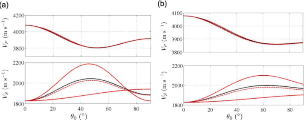
Figure 4.Illustration of the inconsistency of the velocity averaging method for the two VTI textures shown in Fig. 2a and b. The velocitiesVP andVSare reported as functions ofθ0, from the effective medium theory (black curves) and from the velocity averaging method (plain red lines). The dotted red lines show the shear wave velocity from Bennett’s expression, close to the harmonic mean of the two unphysical shear wave velocities in plain red line.
VSHav = s
Lcθ02+N sθ02
ρ ,
VSVav = s
C+L+(A−C)sθ02−√D
2ρ ,
VPav= s
C+L+(A−C)sθ02+√D
2ρ ,
(25)
with
D≡hAsθ02−Ccθ02i hAsθ02−Ccθ02+2Lcθ02−sθ02i +4sθ02cθ02F2+2F L+L2.
These velocities are reported in Fig. 4a (red curves) and they will be discussed later. We now derive the two shear and transverse velocities of the effective medium, Sect. 3.1.2, which are given by Eq. (23) with CeffI J(θ0)=RdθhCI Jiϕ(θ )sinθ Pθ0(θ ), and Eqs. (21)
and (24). We get
Veff P =
r 1 ρ h
Asθ04+2(2L+F )sθ02cθ02+Ccθ04i,
VSeff=
r 1 2ρ
h
(A+C−2F )sθ02cθ02+L
4sθ04−5sθ02+2
+N sθ02 i, (26) and these velocities are reported in black lines in Fig. 4a. 3.2.2 Example 2: the VTI clustered texture with
opening angleθ0
This texture is shown in Fig. 3. It corresponds to
Pθ0(θ )=
Hθ0(θ )
1−cosθ0
, (27)
where Hθ0 is the rectangular function, equaling unity for
0≤θ≤θ0 and zero otherwise. The velocities (VSHav, VSVav,
VPav) in the velocity averaging method, Sect. 3.1.1, cannot
be calculated analytically in this case. The averages onθin Eq. (18) are performed numerically (with Eqs. 17 and 27), and they are shown in red lines in Fig. 4b.
The velocities of the effective medium (VSeff and VPeff; Sect. 3.1.2) are calculated as previously, using Eqs. (21) to (23), with Eq. (27), and we get
Cluster
Veff S =
r (L+N )
2ρ +
[2(A+C)−4F−3L−5N] 30ρ X−
[(A+C)−2(2L+F )] 10ρ Y
VPeff=
r A ρ+
[−7A+3C+4(2L+F )] 15ρ X+
[A+C−2(2L+F )] 5ρ Y
(28) with X≡1+cosθ0+cos2θ0 and Y≡cos3θ0+cos4θ0. These results are shown in black lines in Fig. 4b.
Let us now discuss Fig. 4. Black lines correspond to the velocitiesVPeffandVSeffand as previously said, a unique ve-locity VSeff is found from the effective medium theory, by construction. Red lines correspond to the velocitiesVPav and (VSHav,VSVav) from the velocity averaging method. The discrep-ancy is incidental for the longitudinal wave velocity and does not allow to discriminate between the two methods. The im-portant result is that we find two distinct shear wave veloci-ties using the velocity averaging method, which is unphysical in the present case.
4 Comment on Bennett’s derivation of the velocities in the usual clustered texture
4.1 Bennett’s calculations in Bennett (1968) Bennett starts with the slowness in a single crystal
S=1/V ,
given by
S1=SP≃a1−b1cos 4θ−c1cos 2θ,
S2=SSV≃a2+b2cos 4θ,
S3=SSH≃a3+b3cos 2θ,
(29)
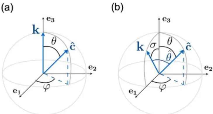
where (a1,a2,a3,b2,b3) are constant for ice. The above ex-pressions are close to the Thomsen approximations (Thom-sen, 1986). They correspond to approximate expressions of the inverses of the velocities for the single crystals as given in Eq. (17). In the above expressions, θ is the angle (k,cˆ) (Fig. 5a). Bennett used a different frame where neitherknor
ˆ
c are along the directione3. In this frame, he defined new multiple angles (Fig. 5b):σ≡(k,e3),θ=(cˆ,e3) andθˆ≡(k,
ˆ
c).
An additional angleϕˆ, not represented in Fig. 5a, between the planes (k,e3) and (k,cˆ) is used. Next, an ensemble of re-lations between the different angles is derived, among which cosθˆ=sinσcosϕsinθ+cosσcosθand
sin2ϕˆ=sin
2ϕ sin2θ
sin2θˆ ,
cos2ϕˆ=(cosσcosϕsinθ−sinσcosθ )
2
sin2θˆ .
(30)
These relations are correct; for instance ifσ=0, thenθˆ=θ
andϕˆ=ϕ, as expected. Next, it is said that the slowness of the wave depends onϕˆfollowing
SP=S1,
SSV=S2cos2ϕˆ+S3sin2ϕ,ˆ
SSH=S2sin2ϕˆ+S3cos2ϕ.ˆ
(31)
This is postulated by Bennett as being an intuitive approx-imation. Since ϕˆ can vary while θˆ remains constant (see Eq. 30), the above equations pretend that the velocity of the shear waves depends on more than just θˆ, which Eq. (29) shows as incorrect. More explicitly, usingσ=0 (thus,θˆ=θ,
ˆ
ϕ=ϕ) in Eq. (31) and using Eqs. (29)–(30), we get
SSV =(a2+b2)−8b2cos2ϕcos2θsin2θ
−2b3sin2ϕsin2θ,
SSH =(a2+b2)−8b2sin2ϕcos2θsin2θ
−2b3cos2ϕsin2θ,
(32)
similarly to Eqs. (5)–(15) in Bennett (1968). These expres-sions for the velocities in a single crystal contain an unphys-ical dependence vs.ϕand they are not in agreement with the original expressions, Eq. (29), they derive from. The modifi-cation performed in Eq. (31), when compared with the orig-inal expressions, consists of attributing symmetrical weights
Figure 5. (a)System of angles used in Bennett’s calculations.cˆis given by (ϕ, θ) andkis given byσ, being otherwise in the (e1, e3) plane. The extra angleθˆ denotes the angle between kandcˆ, thus cosθˆ=sinσcosϕsinθ+cosσcosθ.(b)Particular case of the Bennett configuration, forσ=0; in this case,θˆ=θ.
to bothS1andS2in order to get an identical value for the two shear wave velocities, after velocity averaging. Bennett’s re-sults are reported in dotted red lines in Fig. 4. As expected, the shear wave velocity appears to be close to the harmonic mean of the two unphysical velocities (resulting from the ve-locity averaging calculation). The veve-locity of the P wave, be-ing not modified by artificial weights, remains the same.
It is difficult to anticipate the consequences of such an ap-proach in the case of other textures, since the weights used to deduce the shear wave velocity in Eq. (31) were chosen while anticipating a result expected after velocity averaging. The intuition that one can have for simple texture configura-tion may become hazardous when complex textures are dealt with.
5 Conclusions
In this paper, we have proposed a critical analysis of the ve-locity averaging method that has been used recently in the post treatment of the wave velocities deduced from borehole sonic logging measurements along ice cores. We have illus-trated the error made in the fundamental assumption postu-lated at the basis of this method. This critical analysis is per-formed here in the case of simple VTI textures for which the error leads to an unphysical result and thus allows for a clear demonstration. For VTI textures, Bennett circumvented this problem by postulating weighted forms of the shear wave velocities (Bennett, 1968). The method is clever but it re-quires us to be able to anticipate good guesses for the selected weights, which may become difficult in the case of complex crystallographic textures.
single crystal is weak, and thus the anisotropy of ice poly-crystals is even weaker. On the other hand, ice along bore-holes is reasonably free of impurities when compared to most of the materials studied by similar sonic measurements. The recent sonic logging campaign performed at EPICA Dome C has revealed the feasibility of such measurements (Gus-meroli et al., 2012). Nowadays, commercial loggers measure precisely the velocity. In parallel, the characterization of the physical properties of the ice single crystal and of the de-pendences of these properties with pressure and temperature reaches precisions of the order of a few percents. This in-crease in the precision renders the inverse problem accessi-ble, from the measured velocities to the ice texture, but the inversion model still requires a high level of accuracy. With respect to this requirement, a rigorous model as the model based on the effective medium theory appears as a good can-didate and should be favored.
Acknowledgements. We are thankfull to A. Diez and an anonymous referee for helping to improve the paper. Maurine Montagnat is supported by the French CNRS (Centre National de la Recherche Scientifique) and the institutes INSIS (Institut des Sciences de l’Ingénierie et des Systemes) and INSU (Institut National des Sciences de l’Univers).
Edited by: O. Eisen
Reviewed by: A. Diez and one anonymous referee
References
Azuma, N. and Goto-Azuma, K.: An anisotropic flow law for ice-sheet ice and its implications, Ann. Glaciol., 23, 202–208, 1996. Bennett, H. F.: An investigation into velocity anisotropy through measurements of ultrasonic wave velocities in snow and ice cores from Greenland and Antarctica, PhD thesis, University of Wis-consin, Madison, 1968.
Blankenship, D. D., Bentley, C. R., Rooney, S. T., and Alley, R. B.: Till beneath Ice Stream B: 1. Properties derived from seismic travel times, J. Geophys. Res.-Solid Ea., 92, 8903–8911, 1987. Diez, A. and Eisen, O.: Seismic wave propagation in anisotropic ice
– Part 1: Elasticity tensor and derived quantities from ice-core properties, The Cryosphere, 9, 367–384, doi:10.5194/tc-9-367-2015, 2015.
Gusmeroli, A., Pettit, E. C., Kennedy, J. H., and Ritz, C.: The crystal fabric of ice from full?waveform borehole sonic logging, J. Geo-phys. Res.-Ea. Surf., 117, F03021, doi:10.1029/2012JF002343, 2012.
Kohnen, H.: The temperature dependence of seismic waves in ice, J. Glaciol., 13, 144–147, 1974.
Maurel, A., Lund, F., and Montagnat, M.: Propagation of elastic waves through textured polycrystals: application to ice, P. Roy. Soc. Lond. A, 471, 2177, doi:10.1098/rspa.2014.0988, 2015. Thomsen, G. W.: Weak elastic anisotropy, Geophysics, 15, 1954–
1966, 1986.
Vélez, J. A., Tsoflias, G. P., Black, R. A., Van der Veen, C. J., and Anandakrishnan, S.: Distribution of preferred ice crystal orienta-tion determined from seismic anisotropy: Evidence from Jakob-shavn Isbræ and the North Greenland Eemian Ice Drilling facil-ity, Greenland, Geophysics, 81, WA111–WA118, 2016. Voigt, W.: Lehrbuch der Kristallphysik, reprint of the 1st Edn.,