Deblocking of Interacting Particle Assemblies:
from Pinning to Jamming
M.-Carmen Miguel,
Departament de F´ısica Fonamental, Facultat de F´ısica, Universitat de Barcelona, Av. Diagonal 647, E-08028, Barcelona, Spain
Jos´e S. Andrade Jr.,
Departamento de F´ısica, Universidade Federal do Cear´a, 60451-970 Fortaleza, Cear´a, Brazil.
and Stefano Zapperi
INFM unit`a di Roma 1 and SMC, Dipartimento di Fisica, Universit `a “La Sapienza”, P.le A. Moro 2, 00185 Roma, Italy
Received on 24 April, 2003
A wide variety of interacting particle assemblies driven by an external force are characterized by a transition between a blocked and a moving phase. The origin of this deblocking transition can be traced back to the presence of either external quenched disorder, or of internal constraints. The first case belongs to the realm of the depinning transition, which, for example, is relevant for flux-lines in type II superconductors and other elastic systems moving in a random medium. The second case is usually included within the so-called jamming scenario observed, for instance, in many glassy materials as well as in plastically deforming crystals. Here we review some aspects of the rich phenomenology observed in interacting particle models. In particular, we discuss front depinning, observed when particles are injected inside a random medium from the boundary, elastic and plastic depinning in particle assemblies driven by external forces, and the rheology of systems close to the jamming transition. We emphasize similarities and differences in these phenomena.
I
Introduction
Various materials ranging from synthetic nanocrystals, mag-netic colloids, charged particles in Coulomb crystals, pro-teins and surfactants, or vortices in type II superconduc-tors and in Bose-Einstein condensates, form ordered self-assembled structures. This topic has attracted much interest for various fundamental and technological reasons. In this respect, the response of these structures to external forces of various kinds (optical, magnetic, mechanical) is of particu-lar importance [1-3]. In many cases one observes the pres-ence of blocked phases, where the evolution of the system is frozen. This behavior can have different origins: when it is due to the presence of quenched disorder it is denoted by pinning, while when it is due to intrinsic constraints it is referred to as “jamming”. In both cases, a sufficiently large force leads to a moving phase, through a deblocking transi-tion.
All these systems can be modeled by a set of inter-acting particles moving under the action of external forces sometimes in a random pinning field. For instance, super-conducting vortices in thin films are pinned by vacancies and driven by an applied current through the Lorentz force, colloids interact replace by via Van der Waals or dipolar forces and are driven by the solvent flow. Despite the dif-ferences in these systems, one can try to identify some com-mon features in their dynamic response. This goal has been
achieved mostly through the use of numerical simulations, which have been extensively employed in the past in various contexts. Here we review the results obtained from numer-ical simulations of interacting particles, in order to provide a common framework for pinning and jamming phenomena that, despite their similarities, have been traditionally stud-ied by different communities.
phenom-ena is not so advanced. Similarly, when depinning involves the generation of topological defects, one refers to a plas-tic depinning transition, but the precise meaning of the word transition is not clear at present in this context.
At this stage of the theoretical understanding, however, it is possible to draw an extensive common picture of these phenomena, in which some parts are depicted in full detail, others are less precise, and some are just sketched. We hope that this work, by its own nature incomplete, will stimulate others to find further connections between non-equilibrium transitions from blocked to moving phases and possibly to formulate a complete theory encompassing all these phe-nomena.
The paper is organized as follows: in section II we dis-cuss the models used to describe the physics of interacting particle assemblies. In section III, we analyze the injection of particles in a random medium and discuss the relations with front propagation and with continuum theories. Sec-tion IV is devoted to the depinning of interacting particles by an external force through a pinning field. We analyze the problem by increasing gradually the level of complex-ity, from the pinning of single particle to collective elastic and plastic depinning. In section V, we introduce jamming phenomena and discuss in detail the jamming transition ob-served in plastically deformed crystals, modeled by a set of stress-driven interacting dislocations. We conclude briefly in section VI.
II
Interacting particle models and
their physical realization
Several systems in nature can be modeled by a collection of interacting particles. Here we summarize the main features of these models and discuss some concrete examples. For simplicity, we will restrict ourselves to pairwise interactions between particles. In this case, identifying the particle coor-dinates by~ri, withi = 1, ...N, we can write the equations of motion in general as
md
2~r
i
dt2 + Γ
d~ri
dt =
X
j
~
J(~rj−~ri) +F~ext(~ri, t), (1)
wheremis the mass of the particles,Γis a damping coef-ficient, andJ~ =−∇~V(~r)is the interparticle force derived from an interaction potential V. The last term represents external forces, quenched disorder, or other noise sources, and will be discussed in detail below. In most cases of inter-est, dissipation is so strong that we can safely neglect inertia putting m = 0. Most of the following discussion will be devoted to this overdamped limit, but occasionally we will discuss as well the effect of inertia.
Depending of the particular system under study, the in-terparticle potential can have different forms which will af-fect the dynamics of the system. The simplest case is that of a short-range repulsive central forceJ~(~r) = ˆrK(|~r|/ξv) which can be characterized by its peak valueK(0)and its rangeξv. In a series of increasing complexity, one can con-sider non-monotonic interactions (i.e. the force can be
re-pulsive and attractive in different ranges), long-range inter-actions (i.e. K(r)∼r−α, for largerwith0< α < d+ 2, anisotropic forces (i.e.J~= ˆrK(~r)), non-central forces (i.e.
~
J(~r)×rˆ6= 0), or different combinations of the above. The external force normally includes a uniform driving force F, which could be time dependent. Typical exam-ples are the AC drive F(t) = F0sin(ωt)or the ramp up
F(t) =ct, but the possibilities are endless. In addition, one should consider position dependent forces due to quenched impurities that may be present in the system. Here we will mainly discuss the effect of a set ofNppinning points placed randomly at positionR~p, giving rise to a random force field of the type
Fp(~r) =X p
~
fp((~r−R~p)/ξp), (2)
whereξpis the range of the individual pinning forces. Nor-mally, the particular shape of the pinning potential does not matter as long as its range is short. One can also consider correlated disorder, such as columnar and planar defects, de-pending on the particular situation at hand. In addition, ther-mal effects can be included adding a a random uncorrelated Gaussian termη(~r, t)to the equation.
Once the interactions of the particle systems have been specified, one should also discuss the boundary and initial conditions of the model. A common choice is to use peri-odic boundary conditions, and to place the particles in their zero temperature equilibrium positions (i.e. forming a crys-tal). Alternatively, the particles can be placed randomly in the system mimicking a sudden quench from a disordered high temperature phase. The latter may give rise to an intrin-sic geometrical disorder. These conditions are appropriate if one is interested in modeling the dynamics in the bulk of the material, without worrying about surface effects. On the other hand, boundary effects are at the core of the phenom-ena in some cases and one should then implement different initial and boundary conditions. This case will be discussed explicitly in the next section. Periodic boundary conditions need special care when interactions are long-ranged, since in this case one cannot impose a cutoff to the extent of the interaction force, as it is often done for short range-forces. One should instead consider explicitly the interaction of the particles in a given finite cell with all the periodic images of the system. The infinite sum over the images can rarely be performed exactly and since the sum is slowly converging a simple truncation of the series gives a poor approximation and may induce spurious effects. To overcome this problem one can employ the Ewald summation method, originally proposed for Coulomb interactions, after generalizing it for the appropriate interactions involved [6].
vortex lines. The interparticle force between rigid flux-lines in the framework of the London theory is given by
~
J(~r) = Φ20/(8π2λ3)K1(|~r|/λ)ˆr, (3)
whereΦ0is the quantized flux carried by the vortices,K1
is a Bessel function andλis the London penetration length [28, 27]. Notice that this is a short-range (sinceK1(x) ∼
exp(−x)for largex) repulsive central force, with a diver-gence of the formx−1at short distances which is cut off by
the vortex core. Instead in two dimensions, the interaction is long-range
~
J(|~r|) = Φ
2 0rˆ
8π2λ2r, (4)
decaying as1/r. In addition to interaction forces, a current
~j flowing in the superconductor produces a Lorentz force
~
F =~j×B/c~ acting on the vortices.
In the case of complex fluids or soft condensed matter materials [7], which usually contain large poly-mer molecules or colloidal particles in a solvent whose molecules are much smaller in size, a generic model in which inertial terms are neglected often provides an effec-tive approach towards describing such systems. The solvent is considered as a continuum medium, characterized by its viscosity, in which energy is dissipated as the suspended par-ticles move through it. In close correspondence with their characteristic dissipative motion, the suspended particles ex-hibit a Brownian dynamics due to the random collisions with the solvent molecules. This is modeled as a random Gaus-sian force~ηin the equations of motion of the form
Γi(d~ri
dt −~v
s) =J~(~ri) +~η(~r
i, t), (5) where~vs is the solvent velocity that can be controlled by an externally applied flow field, andJ~is an elastic or con-servative force on particle i due to deformations of long molecules or bubbles, or due to other interactions (such as Van der Waals, electrostatic, magnetic, and excluded-volume) among the suspended particles. The amplitude of the autocorrelation function h|~ηi|2i = 2ΓikBT δ(t−t′) is proportional to the temperature T of the system. More sophisticated algorithms, in which one solves similar equa-tions to the one represented above, have been developed to model the rheology of dense spherical particles [8] account-ing for hydrodynamic interactions, ellipsoidal or rod-like particles [9], as well as emulsions [10] and foams [11].
Another example which is worth considering from this general point of view is a collection of dislocations in a thin crystalline film. Crystal dislocations are topological defects characterized by a Burgers vector~b[12]. As in the case of flux-lines, in a three dimensional crystal dislocations are de-formable lines. Nevertheless, one often treats them in the
rigid approximation, obtaining an effective two dimensional
particle model, which becomes exact for thin samples. Dis-locations produce long-range stress and strain fields in the host crystal, and experience the so-called Peach-Koehler force due to the overall local stress. This induces an interac-tion force between dislocainterac-tions that depends on their charac-ter (edge or screw, when~bis perpendicular or parallel to the
corresponding dislocation axis, respectively [12]), but that is generally long-range, decaying as1/r, and anisotropic. For instance, the force between two edge dislocations at a dis-tance~r= (x, y), and with Burgers vectors in thexdirection is given by
Jx(x, y) = µb
2
2π(1−ν)
x(x2−y2)
(x2+y2)2, (6)
whereµis the shear modulus, andν is the Poisson ratio of the host crystal. We have only considered thexcomponent since, differently from flux lines, dislocations move mainly by gliding along preferential directions, namely the direc-tion of the Burgers vector. Thus, while the particle system is two dimensional, the motion is confined along several par-ticular directions. This fact, together with the anisotropic character of the interaction, gives rise to metastable struc-tures that act as geometric constrains for their own dynam-ics. In this case, the driving force is often an externally applied stressσwhich acts on the dislocations through the Peach-Koehler forceF~ = (~b·σ)×Lˆ, whereLˆis the direction of the dislocation line local tangent.
III
Gradient driven dynamics: front
invasion
The theoretical and experimental investigation of the growth dynamics of rough interfaces has became a subject of great scientific interest in recent years [13-15]. This is clearly illustrated nowadays by the large variety of studies deal-ing with front invasion where roughendeal-ing processes take place such as flow through porous media [16-18] or imbibi-tion [19], flame propagaimbibi-tion [20, 21], deposiimbibi-tion processes [14, 15], and flux penetration in superconducting materials [32, 33, 45, 46].
transport in self-similar (fractal) structures usually occurs in the form of a subdiffusive regime [25, 26].
The invasion of magnetic flux into a disordered type II superconductor is another problem that has recently been the object of intense theoretical and experimental research. As a matter of fact, the magnetization properties of type II super-conductors have been studied for many years, but the inter-est in this problem has been renewed with the discovery of high temperature superconductors [27, 28]. The magnetiza-tion process is usually described in terms of the Bean model [29] and its generalizations: flux lines enter into the sam-ple and, due to the presence of quenched disorder, give rise to a steady flux gradient. While the Bean model provides a consistent picture of average magnetization properties, such as the hysteresis loop and thermal relaxation effects [30], it does not account for local fluctuations in time and space. It has been recently observed that flux line dynamics is inter-mittent, taking place in avalanches [31], and flux fronts are not smooth [32-34]. In particular, it has been shown that the flux front crosses over from flat to fractal as a function of material parameters and applied field [33].
A widely used modeling strategy to describe the fluc-tuations around the Bean state consists of numerical simu-lations of interacting vortices, pinned by quenched random impurities [35-40]. With this approach it has been possible to reproduce flux profiles [37], hysteresis [37], avalanches [36, 39, 40] and plastic flow [35, 40]. One of the aims of these studies [37] is to establish precise connections be-tween the microscopic models and the macroscopic behav-ior, captured for instance by generalized Bean models. A different approach treats the problem at mesoscopic scale, describing the evolution of interacting coarse-grained units [41, 42], supposed to represent the system at an intermediate scale. While these models give a faithful representation of several features of the problem, the connection with the un-derlying microscopic dynamics still represents a very active field of research.
A. Invading front from an interacting particle simulation
In this section, the main objective is to show that the gradient driven dynamics of the overdamped motion of in-teracting particles in disordered substrates can display a col-lective behavior that is typical of front invasion processes with roughened interfaces. More precisely, as we show next, the idea is to provide a basic description for these system in terms of a particle model and to indicate how the relevant scaling laws relating the front position and the flux profile to the pinning strength can be consistently extracted from numerical simulations. The equation of motion for an inter-acting particle performing an overdamped motion in a ran-dom pinning landscape can be written as in Eq. 1
Γ~vi= X
j
~
J(~ri−~rj)+ X
p
~
fp[(R~p−~ri)/ξp]+η(~ri, t), (7)
whereΓis the effective viscosity, the first term on the right hand side represents the particle-particle interaction, and the second accounts for the interaction between particles and pinning centers. Here we consider thatJ~is a short-range interaction, andf~pis the force due to a pinning center, mod-eled as a localized trap at the positionR~p, withξpbeing the range of the wells (typicallyξp≪λ), andp= 1, ..., Np. For example, the pinning force could be modeled in terms of the expression,G~(~x) = −f0~x(|~x| −1)2, for|~x| < 1and zero
otherwise. For completeness, an uncorrelated thermal noise termηwith zero mean and variancehη2i=k
bTΓδ(t−t′) is also added to the equation, but we will restrict ourselves to the analysis of the caseT = 0(see Ref. [43] for the im-plementation of thermal noise in simulations).
For gradient driven systems, the solution and interpreta-tion of the MD model is essentially accomplished by the si-multaneous numerical integration of Eq. (7) for each moving particle in the system, and subsequent analysis of the flux front propagation for different values of the pinning strength
f0. For instance, one typical simulation [46] can involve
up toNp = 800 000Poisson distributed pinning centers of width ξp = λ/2 in a system of size (Lx = 800λ, Ly = 100λ), corresponding to a density ofn= 10/λ2. The
num-berNof flux lines depends essentially on the boundary con-dition adopted in the simulation. The injection of particles into the sample is implemented through the concentration at
t= 0of all particles in a small sliceL′≪λ, parallel to the
y direction, and imposing periodic boundary conditions in both directions. Due to mutual repulsion in the dense zone of the slice, the particles will be pushed inside the material, forming a penetrating front. The front position can then be taken as thexcoordinate of the most advanced particle in the system at different times, or one can divide the system into a grid and identify the front (see Fig. 1).
B. Non-linear diffusion
Now we show that the front penetration due to the col-lective motion of interacting particles in a substrate of pin-ning centers can be described by a disordered non-linear dif-fusion equation [51]. The equation can be obtained perform-ing a coarse-grainperform-ing of Eq. (7), startperform-ing from the Fokker-Planck equation for the probability distribution of the flux line coordinatesP(~r1, ...., ~rN, t)
Γ∂P
∂t =
X
i
~
∇i(−f~iP+kBT ~∇iP), (8)
where f~i is the force on the particle i given by Eq. (7). Next, we introduce the single particle density ρ(~r, t) ≡ hP
0 50
y
100 150 050 100 150
x
1 10 100 1000 10000 100000
t
10 100 1000
x
pf0=0.01 f0=0.02 f0=0.04 f0=0.06 f0=0.10
Figure 1. In the upper panel we show a typical realization of a flux front obtained from a simulation of interacting vortices in a disordered landscape [46]. In the lower panel, we show the growth of the average front position as a function of time for different pinning force strengths. The front initially grows ast1/3
and then is pinned at a distance that scales withf0.
Γ∂ρ
∂t =−∇~
à Z
d2r′J~(~r−~r′)ρ(2)(~r, ~r′, t) +X
p
~
fp[(R~p−~r)/ξp]ρ(~r, t) !
+kBT∇2ρ, (9)
⌈
where ρ(2)(~r, ~r ′, t) is the two-point density, whose
evo-lution depend on the three-point density and so on. The simplest truncation scheme involves the approximation
ρ(2)(~r, ~r ′, t) ≃ ρ(~r, t)ρ(~r ′, t). We then coarse grain the
equation considering length scales larger thanλ. This can be done expandingJ~in Fourier space, keeping only the lowest order term in~q, and retransforming back in real space. The result reads
Z
d2r′J~(~r−~r′)ρ(~r′, t)≃ −a~∇ρ(~r, t), (10)
wherea≡R
d2r~r·J~(~r)/2.
The coarse graining of the disorder term is more subtle. A straightforward elimination of short wavelength modes would give rise, as in the previous case, to a random force
~
Fc(~r) =−g ~∇n, wherenis the coarse grained version of the microscopic density of pinning centersˆn(~r) ≡P
pδ2(~r−
~
Rp)andg∝f0. This method can not be applied for
short-range attractive pinning forces as the one we are investigat-ing. In this case, short wavelength modes yield a macro-scopic contribution to pinning that can not be neglected.
Consider for instance the flow between two coarse grained regions: short-range microscopic pinning forces give rise to a macroscopic force that should always oppose the mo-tion, while the random force derived above could in prin-ciple point in the direction of the flow. In other words,
Fc(~r)should be considered as a friction force whose direc-tion is always opposed to the driving forceF~d(in our case
~
Fd=a~∇ρ) and whose absolute value is given by|g ~∇n|for |F~d|>|g ~∇n|and to|F~d|otherwise [44].
Collecting all the terms, we finally obtain a disordered non-linear diffusion equation for the density of particles
Γ∂ρ
∂t =∇~(aρ~∇ρ−ρ ~Fc) +kBT∇
2ρ. (11)
specific, we consider the situation in which the front pen-etration takes place in a disordered type II superconductor and the particles are vortices interacting according to Eq. (3) [46, 45]. The following BC’s correspond to different exper-imental situations [47, 48]:
• (A) Constant total number of vortices. Experimen-tally this corresponds to an external control of the magnetic flux.
• (B) Constant vortex concentration at the boundary. This case corresponds to an external control of the magnetic field.
• (C) Total vortex number increasing at constant rate. This represents an external control of the flux rate. • (D) Boundary concentration increasing at constant
rate, corresponding to a constant field rate.
One should notice that boundary conditions can be more complicated in reality, due to complex surface barriers that oppose flux penetration.
For a clean system (f0 = 0) atT = 0, Eq. (11) can be
solved exactly using scaling methods [47, 48]. In this case, the density profiles obey the equation
ρ(x, y, t) =t−χ
G(x/tψ), (12)
whereχandψsatisfyχ+ 2ψ = 1. For the BC’s consid-ered: A) χ = 1/3, ψ = 1/3; B) χ = 0, ψ = 1/2; C)
χ =−1/3,ψ = 2/3; and D)χ = −1,ψ = 1. These ex-ponents are in perfect agreement with the results from MD simulations reported in Ref. [46]. For instance, the data re-ported in Fig. 1 correspond to boundary condition (A) and correctly scale withψ = 1/3. The functionG(u)also de-pends on the boundary condition and for the case (A) is given byG(u) = (1−u2)/6 foru < 1 and vanishes for
u≥1. The other cases are reported in Refs. [47, 48]. The presence of disorder (pinning centers) induces sub-stantial effects on the behavior of the system that can be quantified in terms of the front propagation and/or the shape of the density profiles of flux lines. Depending on the boundary conditions, it has been observed that the front is either pinned or simply slowed down [45]. Extensive numer-ical simulations have also been performed in Refs. [45, 46] to show the compatibility between the MD model with dis-order and its coarse-grained representation, Eq. (11). More-over, by varying the parameters of this continuum descrip-tion of the front propagadescrip-tion, a crossover from flat to fractal flux fronts has been detected, consistent with experimental observations. The value of the fractal dimension suggests that the strong disorder limit is described by percolation. In the weak disorder limit, we recover the analytical results de-rived in Refs. [47, 48].
IV
Externally driven dynamics:
de-pinning and flow
In this section, we discuss the response of interacting parti-cles to an external force in presence of quenched disorder.
The effect of quenched disorder is first analyzed in a sin-gle particle model, which, although oversimplified, still dis-plays a depinning transition. The effect of the interparticle potential on the depinning transition will be first introduced in the framework of the elastic theory, which breaks down for strong pinning, leading to plastic depinning. Finally, we briefly discuss the moving phases observed for strong driv-ing.
A. Single particle pinning
A first understanding of the dynamics of driven particles in a disordered landscape can be obtained considering the motion of a single particle [49-51]. We consider a collec-tion of parabolic wells for the pinning potentials, so that the equation of motion for a single particle is given by
Γdx
dt =F+
X
p
f0(Xp−x)θ(|x−Xp| −ξp), (13)
where are the random coordinates of the pinning centers, which we assume to be non-overlapping. When the particle is not interacting with a pinning center, it moves with con-stant velocity F/Γ, until it enters into the attraction range of a pinning center. Considering this as the initial condition (i.e.x(t= 0) =Xp−ξp), we can solve the equation
Γdx
dt =F+f0(Xp−x) x < Xp+ξp, (14)
which is given by
x(t) =Xp+F/f0−(F/f0+ξp)e−t/Γ. (15)
In the limit t → ∞ the particle remains trapped as long asF < Fc =ξpf0and escapes otherwise. We can interpret
this behavior as a depinning transition: the particle is pinned forF < Fcand moves forF > Fc.
The force-velocity diagram can be computed noting that forF > ξpf0the particle spends in each trap a time
τ = Γ log((F+Fc)/(F−Fc)). (16) The total timeT to cross a system of lengthLwithNp pin-ning centers is given by
T =Npτ+ (L−2ξpNp)Γ/F. (17) The average velocity of the particle is thus given by
v= L
T =
F
Γ(F nplog((F+Fc)/(F−Fc)) + (1−2ξpnp))
,
v∼(F−Fc)1/2[50]. We notice that the dependence of the exponents on the pinning potential is a peculiarity of the sin-gle particle behavior and is not observed when interactions come into play as we will discuss in the next section.
Single particle models are also useful for gradient driven dynamics discussed in the previous section [46]. In that case the external forceF is replaced by the density gradi-ent, which can be approximated with a simple function of
x. For instance, in the case of boundary condition (B) (see section III)F ∼ ∇ρ∼ρ0/x, whereρ0is the boundary
den-sity. This simple model yields the correct scaling behavior for the front position [46].
B. Elastic depinning
In the previous section, we have only considered the in-teractions between moving particles and static pinning cen-ters. We could expect that those results will be valid only when the interactions between particles can be neglected,
as for instance in a very dilute system. In most situations, however, interactions between particles should be explicitly taken into account. In this case we will still observe a depin-ning transition, but its quantitative and qualitative features will change [52-58]. It is convenient to first study an inter-acting particle system in the elastic approximation, in which the pinning forces are not strong enough to break the topo-logical properties of the particle system. For instance, if the particles are arranged into a crystal, the external force and the disorder preserve the topological order and no defects are generated.
In the pinned phase we can write the positions of the par-ticles by their displacement vectors~u(R~i) =~ri−R~i, where
~riare the coordinates in the deformed system andR~iare the equilibrium positions. The particle interaction energy can then be expanded in terms of the displacement field, which is assumed to be small,
⌋
U =X ij
V(~ri−r~j)≃U0+ X
α,β X
ij
(uα(R~i)−uα(R~j))
∂2V
∂rαrβ
(uβ(R~i)−uβ(R~j)), (19)
⌈
whereU0 is the energy in equilibrium. One can then take
the continuum limit expanding in small gradient u(R~) ≃
u(R~′) + (R~ −R~′)·∇~u(~r)and obtain [59]
U =U0+1
2 Z
d3r X
α,βγδ
Eα,βγδ∂uα
∂rγ
∂uβ
∂rδ
, (20)
where the elastic tensorEα,βγδcan be expressed in terms of the interparticle pair potential as
Eα,βγδ=−1 2
X
R
RγRδ ∂
2V
∂rαrβ
(21)
Clearly this expansion holds as long as the sum in Eq. 21 converges. If interactions are long range, decaying with a slow power lawV(r)∼r−(d−1+σ)withσ <2, the elastic
energy can not be expanded in gradients and we have to live with a non-local interaction.
Coming back to the local limit, a further simplification is obtained in Eq. (20) if we take into account the symmetries of the equilibrium system. In the case of an isotropic system, the elastic tensor has only two independent components and the energy reduces to
U =U0+1
2 Z
d3rK
µ
∂uα
∂rα ¶2
+µ
µ
∂uα
∂rβ ¶2
, (22)
whereKandµare the compression and shear moduli, re-spectively.
Using the elastic expression for the interparticle energy, we can rewrite the equation of motion for the particles as
∂uα
∂t =µ∇
2u
α+(K+µ)
∂ ∂rα
(∇·~ ~u)+F+fα(r, u). (23)
When expanding around a moving state, we obtain the same equation with an extra convective term~v·∇~uon the left hand side [60, 61]. These elastic equations are still impossible to solve exactly, but several results have been obtained using scaling theories and renormalization group calculations [52-58]. In the case of long-range interactions the gradients are replaced by a non-local interaction kernel and the equation becomes
∂uα
∂t =
Z
ddr′Kαβ(r−r′)(uβ(r′)−uβ(r))+F+fα(r, u),
(24) withKαβ(r)∼1/rd+σfor large distances.
A first insight on the behavior of interacting particles in a disordered media in the elastic approximation can be gained by collective pinning theory, originally due to Larkin [62]. In this approach, the main energetic contributions en-tering the problem are written as a function of a lengthscale
L. Minimizing the sum of elastic and disorder energies, one obtains the characteristic length Lc at which pinning becomes relevant. Considering a region of sizeL, where the typical displacements of the elastic medium are of the order of the range ξp of the pinning potential, the elastic energy can be estimated asEel ∼µLd−2ξp2, where for sim-plicity we have only considered the shear modulusµ. The pinning energy can be estimated in the limit of weak pin-ning, when the main effect comes from the fluctuations in the disorder: in a region of sizeL, the typical fluctuations of the pinning energy scale asEpin∼ −Ep
p
Ldn
p, where
energyµLd−2ξ2
p−EppLdnpwith respect toL, we obtain the Larkin length
Lc∼ Ã
µξ2
p √n
pEp !4−2d
. (25)
ForL < Lc the elastic medium is essentially undeformed, while elastic deformations grow strongly forL > Lc and typically, the system becomes rough on large lengthscales.
Notice that the Larkin length decreases with the disorder strength as long asd < dc = 4. The dimensiondc = 4 en-ters here for the first time, but has in fact a great importance. As can be shown by renormalization group calculations,dc is the upper critical dimension: ford > dc the system does not roughen and the critical behavior at the depinning transi-tion is essentially mean-field like. Since the physical dimen-sion is usually lower than four, one is lead to think that this limit is without practical interest. This is not completely true, since in presence of long-range interactionsdc typi-cally lowers, reaching sometimes the physical dimension. In particular, for non local elastic interactions withσ < 2 the upper critical dimension is given bydc= 2σ.
Since Lc represents the characteristic lengthscale at which pinning starts to be effective, Larkin estimated the depinning threshold as the force needed to unpin a region of lengthLc. This can be done comparing the energy due to the external forceEext = F ξpLd to the pinning energy at the scaleLc, obtaining
Fc ∼Ep√npL−cd/2/ξp=
(fp√np)4/(4−d) (ξpµ)d/(4−d)
. (26)
Collective pinning theory provides a qualitative descrip-tion of the depinning transidescrip-tion and a good estimate of the depinning threshold, but does not allow to estimate the crit-ical exponents and the force-velocity curve. For this, one needs renormalization group methods, which we do not want to discuss here. We just quote some results, obtained for the first order in aǫ = 4−dexpansion: the exponent for the velocity scaling is given byβ = 1−ǫ/9, while the roughness exponent, ruling the scaling of the typical dis-placements with the system sizeu ∼ Lζ, is estimated as
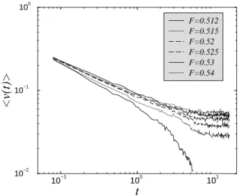
ζ = ǫ/3. Other exponents follow from scaling relations. For instance, one can analyze the transient behavior of the average particle velocity, which initially decays as a power law hvi ∼ t−α, and then crosses over to a constant value whenF > Fc, or goes exponentially to zero otherwise (see Fig. 2) [51]. The exponentαcan be obtained by a scaling relation asα=β/νz, wherezis the dynamic exponent and
νis the correlation length exponent [51].
Simulations have been widely used in the past to obtain numerically the value of the exponents. We should distin-guish here the vast body of work pertaining to elastic mani-folds, in which the elastic approximation is enforced directly in the model simulating variants of Eq. 23 [55], from particle simulations in which the original system is studied. In one dimension the elastic approximation works well and the ex-ponents measured in particle models reproduce with a good accuracy the results obtained for elastic manifolds, namely
β ≃ 0.25 andζ ≃ 1.25(see Fig. 3) [51,63-65]. This is
not surprising since in d = 1topological order is trivially present. In two dimensions from the mapping with elastic manifold we would expectβ ≃0.65andζ≃0.75[55] and at least the first exponent is reproduced by particle simula-tions [66].
10−1 100 101
t
10−2
10−1
100
<v(t)>
F=0.512 F=0.515 F=0.52 F=0.525 F=0.53 F=0.54
Figure 2. The decay of the velocity forN = 400interacting par-ticles with pinning ind= 1for different values of the force. For F > Fc= 0.514the velocity crosses over to a steady value. See
Ref.[51] for details on the model.
0.51 0.52 0.53 0.54 0.55
F
0 0.02 0.04 0.06
<v>
Figure 3. The force velocity curve obtained from the steady state velocity shown in Fig. 2. with pinning ind= 1. The best fit yields β= 0.22andFc= 0.514[51].
C. Plastic depinning
When pinning forces become stronger and/or pinning centers more dilute the topological order of the system typi-cally breaks down. In this case, it is not possible to describe the deformation in terms of a displacement field as we did in the previous section, and plastic deformation should be ex-plicitly considered. Due to these difficulties, a complete the-oretical understanding of plastic depinning is still not avail-able and one should rely on numerical simulations. A sim-ple estimate of the conditions for the occurrence of strong pinning effects can be gained in the framework of collective pinning theory. WhenLc∼a0, wherea0is the interparticle
−0.025 0 0.025 0.05 0.075 0.1
v
0 50 100 150 200
P
(v
)
F=0.2 F=0.3 F=0.4 F=0.5
0 0.02 0.04 F
0 0.02 0.04 0.06
<v>
0 0.01 0.02 F 0.03
0 0.2 0.4 0.6 0.8
<n>
v of cutoff to determine n
(a)
(b)
(c)
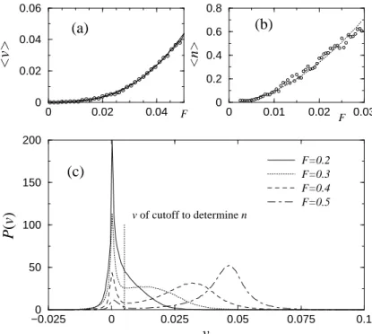
Figure 4. (a) The force velocity curve forN = 270interacting particles in the strong pinning limit ind = 2. The fit is a power lawFβ
withβ= 2.7. (b) The velocity distribution for the same system for different values of the force. Notice the bimodal structure that can be used to set a threshold and identify moving particles. (c) The average number of moving particles scaling with the applied force asFγwith γ= 1.8.
elaborate these type of arguments and draw phase diagrams in terms of disorder and applied force [67].
Here we discuss the main features of plastic depinning as observed in numerical simulations. Typically the force ve-locity curve differs drastically from the one observed when depinning is elastic, which is upward convex (see Fig. 3). In plastic depinning, the curve is convex downward imply-ing thatβ > 1. For instance Ref. [66] findsβ = 2.2 in a simulation of colloids. Others do not provide a value forβ
since it appears that a precise estimate of the exponent is not straightforward [67]. The main reason is that the depinning forceFcis small and one could as well believe thatFc = 0 for a large system, and that the pinning seen in simulations could be an artifact of finite sizes. For instance, the curve reported in Fig. 4 can be reasonably fit as v ∼ Fβ, with
β ≃ 2.7. A small value of Fc would not change signifi-cantly this fit but it is difficult to discriminate between the two cases.
The important differences between plastic and elastic depinning can be highlighted computing the velocity dis-tribution of the moving particles. In plastic depinning the solid breaks apart: some particles are pinned by the strong defects while others move, typically in channels. Thus the velocity distribution develops two peaks: one around zero corresponding to pinned particles, and one at higher veloc-ities [67]. Using this bimodal distribution, it is possible to identify the fraction of moving particleshnmi, using a ve-locity threshold situated in the middle of the two peaks (see Fig. 4). Again the data are reasonably fit by a power lawFγ
withγ≃1.8.
The channel structure of the dynamics has been studied thoroughly in the literature analyzing the statistical
proper-ties of particle trajectories [35, 40, 71]. In Fig. 5 we report an example of the trajectories in the plastic regime, showing the separation between pinned and moving particles. It is also possible to analyze the tearing of the lattice studying its topological properties (i.e. the presence of defects, such as dislocations) [67, 71, 72].
Figure 5. An example of particle trajectories in the plastic regime. Particles are depicted by circles, pinning centers by stars and tra-jectories by lines.
a two dimensional rotated square lattice. When the number of particles present in a site is larger than a threshold, one particle is transferred to a neighboring site. The flow is di-rected and the outlet of each site is random but fixed. It is interesting to note that this model is equivalent to a sand-pile model [76, 77], namely a random (quenched) directed Manna model [78, 79]. It should be possible to use the re-sult obtained for the directed Manna model to solve exactly this model [80, 81]. The model displays a plastic depin-ning transition: some particles are trapped and others flow in channels. The number of particles belonging to the flow basin scales asnm∼(F−Fc)γ, withγ≃0.5. The average particle current (or velocity) scales instead asv∼(F−Fc)β withβ = 1.5. It was conjectured thatβ = 1 +γ, implying that the velocity exponent is due to the combination of the scaling of the velocity of the flowing particlevf and the one of the channel size.
A similar reasoning was proposed in Ref. [75] for plas-tic depinning in a disordered XY model. In this model each spin depins as a single particle in a smooth pinning potential asvs ∼(F −Fc)1/2. The number of spins depinning also scale with the applied force asnm ∼(F −Fc)γ, yielding
β=γ+1/2. The exponentγwas found to be close tod, the dimension of the lattice, which suggests that a simple geo-metrical description could be possible. We notice that the results presented in Fig. 4 satisfy approximately the relation
β= 1 +γ, althoughFc≃0.
Recently, a different approach for plastic depinning was discussed in Refs. [68, 69] through a model of a viscoelastic medium. In this model, depending on the parameter val-ues, one observes first order type or continuous depinning. The model can be approached by mean-field theory [68] and renormalization group [69], but at present the connections with plastic depinning in particle systems is not clear. It is interesting to notice that a first order depinning transition, with hysteresis, is also expected in presence of inertia [70]. Raising the force from the pinned phase towards the moving phase is different than decreasing it when the system is al-ready moving. In the latter case inertia will keep the system in motion even beyond the “depinning threshold”, resulting in an hysteretic force velocity curve.
To summarize, plastic depinning is characterized in gen-eral by the tearing of the elastic medium through the produc-tion of dislocaproduc-tions. Only a fracproduc-tion of the particles move along channels, while the others are pinned, suggesting to interpret the force velocity curve by a combination of scal-ing of sscal-ingle particle velocities and channel size. However, the wide fluctuations of the numerical values for the expo-nents present in the literature and the lack of a theory does not allow a clear quantitative picture of the phenomenon. D. Moving phases, hysteresis and avalanches
When the external driving force is large enough, parti-cles enter into a moving phase which can be of several kinds depending on the type of disorder and the structure of the particle system. All these aspects are reviewed in Ref. [82]. A first understanding of the dynamics of an elastic system for strong driving forces comes from a high velocity expan-sion [83]. When the system flows rapidly one can write
u(r, t) ≃ V t+δu, whereV is the average flow velocity.
In a first approximation the pinning force becomes effec-tively a thermal like noise fp(r, u) ≃ fp(t, V t), with an effective dynamic temperature decreasing with velocity as
Td ∼ 1/V. Thus one would expect that beyond a certain velocity the elastic system would reorder since the effect of pinning forces disappear. The discreteness and period-icity of a particle system modifies considerably this picture: while the displacements along the direction of motion do not feel the disorder due to the high velocity, this is not the case for transverse displacements. Taking into account this effect, Giamarchi and Le Doussal [60] show that the sys-tem should decouple in elastic channels and predict the ex-istence of threshold for transverse depinning. These features have been then observed in simulations [72]. For an exten-sive discussion of other aspects of the dynamics we refer to Ref. [82]
So far we have only discussed the dynamics of interact-ing particles in random media occurrinteract-ing under a constant applied force. When the applied force is time dependent we observe other interesting phenomena. In particular, an AC drive leads to hysteresis, which has been studied in de-tail for domain walls in ferromagnetic materials [85, 86], it should be possible to carry over these results to a generic elastic system with disorder [87]. Hysteresis is expected in the quasistatic limit already at the level of a single particle model driven by an elastic spring [44]. Close to the depin-ning transition, the hysteresis loop of the average displace-ment as a function of the force can be obtained analytically solving the equation [85]
Γhdu/dti= (F0sin(ωt)−Fc)βθ(F−Fc). (27)
Finally, Ref. [88] shows that the velocity force curve also displays hysteresis, but only in the dynamic regime (i.e. hys-teresis is lost in the limitω→0when one recovers the usual force velocity depinning curve).
It is now well established that when the force is raised slowly towards the depinning threshold the dynamics of an elastic system takes place in the form of avalanches as in self-organized criticality [76]. In particular, the avalanche size distribution scales as
P(s) =s−τf(s/s∗), (28)
where the cutoff size grows as a power law with the dis-tance from the critical points∗ ∼ (F
c −F)−νD. Hereν is the correlation length exponent and D is the fractal di-mension of the avalanche (i.e. s∗ ∼ ξD ) whereξ is the correlation length. The connection with self-organized crit-icality is more apparent when the elastic system is driven at “constant velocity” [65]. This can be achieved coupling the system elastically to a slider moving at constant velocity, or, in other words, replacingF byk(V t−R
V
Kinetically constrained dynamics:
jamming and shear yielding
In this section, we will discuss the flow behavior of a wide class of physical systems whose dynamics is governed by the presence of kinematical constraints induced by both in-teractions and geometry. One of the main features shared by their dynamics is the presence of jamming, a new concept recently proposed to refer to the suppression of the temporal relaxation of a physical system and its corresponding abil-ity to explore the space of configurations [89, 90]. Under the action of externally applied shear stresses, these systems eventually yield and are able to flow like a viscous fluid. Shear yielding is thus another feature they have in common. As we will see in the following subsections, under stress conditions both soft materials [7] and crystalline solids [91] are susceptible to display jamming and shear yielding, due to the interactions and spatial arrangement of their con-stituent particles in the case of soft-matter systems, or to the interactions and spatial arrangement of their topologi-cal defects—such as dislocations—in plastitopologi-cally deforming crystals. Jamming and yielding could in turn be responsible for the remarkably similar creep and stationary flow rheol-ogy observed experimentally in these systems, in spite of the big differences among the materials involved.
A. Jamming and viscoelastic flow in soft condensed mat-ter mamat-terials
The phenomena of jamming and yielding control the be-havior and properties of soft materials as diverse as colloidal suspensions [92], emulsions [93], foams [94], gels [95, 96], pastes [97], biological tissues [98], and other soft matter systems. Most of these physical systems consist of vari-ous types of soft particles closely packed into an amorphvari-ous state. At such high concentrations, the individual motion of particles is drastically constrained and, as a consequence, soft and concentrated materials usually respond like elastic solids upon the application of low stresses. On the other hand, they flow like viscous fluids above the so-called yield stress valueσy, exhibiting a common rheology. The defor-mation process of amorphous polymeric materials has, for instance, received a great deal of attention [7]. The creep compliance curve of amorphous polymer networks above the glass transition temperature has been reported to closely exhibit the following behavior [99, 100]
J(t) =γ/σ=j0+Ct1/3+t/η, (29)
where γ is the global strain of the material, σ is the ex-ternal stress, j0 is the instantaneous elastic component of
the compliance, and η is the viscosity. According to this behavior, the Ct1/3 term, also known as Andrade creep
term, dominates for times much smaller than the relaxation timetc characteristic of the complex fluid, while a macro-scopic viscous flow of the formt/ηis established after much longer timest >> tc. One can define and measure a time dependent effective viscosity in the Andrade creep regime
η = σ/γ˙ ∼ t2/3, which reaches its equilibrium value at
longer times.
A common nonlinear rheology is also observed for higher stress values, or shear strain-rate values in the case of constant strain-rate experiments which are in most cases per-formed in this class of systems. The stress-strain relation-ships in the steady state are often described by phenomeno-logical equations of the form σ = σy +aγ˙n [101, 102], which imply a nonlinear dependence of the stressσon the shear strain rateγ˙. For a Newtonian dispersionσy = 0and
n= 1, resulting in a constant viscosity coefficientη=σ/γ˙. If insteadσy 6= 0, the equation describes a Bingham fluid. Whenn <1the relation is known as the Hershel-Bulkeley law, but ifσy= 0, the equation describes a power-law fluid, with a shear strain rate decreasing viscosity.
Although the understanding of yield and viscoplastic flow in these materials is difficulted by the absence of a clear mediating mechanism, such as the motion of dislo-cations in a crystal, it has been argued that the common rheology displayed by these general class of complex flu-ids might be attributed to two particular shared properties of these materials: structural disorder and metastability; which are characteristic features of an underlying glassy dy-namics [103]. In a few words, a glassy dydy-namics is asso-ciated to the slow structural relaxation which takes place when some parts of the system are trapped by their neigh-bors and have to surmount large energy barriers to explore further more favorable configurations. Molecular dynam-ics simulations [104, 105, 106, 107] of glass-forming liq-uids and polymers have proved of much help in this re-spect. About the same time, a general “jamming” scenario was also proposed [89] as a common framework to under-stand the mechanical behavior of a broader class of non-equilibrium physical systems (colloidal suspensions, super-cooled liquids, foams, etc. and granular media) which, in spite of their differences, exhibit common properties such as slow dynamics and scaling features near the so-called jam-ming threshold.
Regarding the slow relaxation dynamics characteristic of soft glassy materials, recent experiments [108, 109] show the necessity of incorporating dynamical heterogeneities for its complete description. In this respect, a new light scatter-ing method, introduced in Ref. [96], allowed to detect the intermittent dynamics of a gel formed from attractive col-loids. The dynamics is found to be intermittent due to ran-dom rearrangements which appear to be localized in time. This and similar experiments strongly suggest that intermit-tent behavior seems to be a fundamental ingredient for the slow relaxation in jammed materials.
Finally, it is interesting to point out that an empirical relation known as the “Cox-Merz rule” [110] quite success-fully relates the non-linear steady rheology with the linear but frequency dependent rheological properties of polymer melts. In particular, the Cox-Merz rule relates the steady vis-cosity at a given shear rateγ˙, to the modulus of the dynamic viscosity at a frequencyω = ˙γ, i.e. η( ˙γ) = |η∗(ω)|.
Sev-eral works have a posteriori tried to theoretically justify this empirical relation starting from basic assumptions [111]. Indeed, the time dependent rheology which follows from Eq. (29) in the Andrade regimeη = σ/γ˙ ∼ t2/3, is
˙
γ−2/3reported in Ref. [106] for the steady nonlinear
rheol-ogy of a binary Lennard-Jones mixture, and it would be con-sistent with the Cox-Merz rule forw= 1/t. The shear thin-ning exponent could also be related to the subaging behavior observed in many soft-glassy materialsη∼tµ
w, wheretwis the so-called waiting time andµ <1[112].
In the following section, we will show that most of the attributes discussed for the case of amorphous soft-glassy materials are also shared by crystalline materials like soft metals or vortex lattices deforming plastically due to the mo-tion of dislocamo-tions.
B. Dislocation jamming and viscoplastic creep deforma-tion
The viscoplastic deformation of crystalline solids is due to the creeping motion of dislocations driven by an exter-nally applied stress [113, 114, 12, 115]. The study of the dynamics of these linear topological defects is a subject of considerable interest because of its practical importance in materials design and engineering. It is also interesting from the theoretical point of view for the many features that dis-location motion shares with other complex systems like, for instance, flux lines in high temperature superconductors, or some of the soft matter materials discussed above.
At the beginning of the XX century, Andrade reported that the creep deformation of soft metals at constant temper-ature and stress grows in time according to a power law with exponent1/3, i.e. γ ∼t1/3whereγis the global strain of
the material [116]. More generally, the creep deformation curve usually follows the relationγ(t) =γ0+βt1/3+κt,
whereγ0is the instantaneous plastic strain,βt1/3is known
as Andrade creep, and κt is referred to as linear creep regime [113, 114]. The same qualitative behavior has since been observed in many materials with rather different struc-tures leading to the conclusion that this should be a pro-cess determined by quite general principles, independent of most material specific properties. Notice that the creep curve for amorphous polymer melts introduced in the previ-ous subsection, follows exactly the same relation. Variprevi-ous arguments have been proposed within the dislocation liter-ature [113,114,117-119] to try to explain Andrade’s creep. Most of them are based on thermally activated processes over time (or strain) dependent barriers, however, there is still a lack of consensus on the basic mechanism involved in the phenomenon.
As in the case of soft-matter systems, the plastic defor-mation of crystals only occurs when the externally applied stress overcomes a threshold value, the yield stress of the material. Above this threshold value, large-scale disloca-tion modisloca-tion may take place, and a steady regime of plastic deformation is eventually established. Dislocations tend to move cooperatively under the action of external stress due to their mutual long-range and anisotropic elastic interactions, which can be attractive or repulsive. As a result of these in-teractions, and of the spatial dislocation structures they give rise to, self-induced constraints build up in the system and the motion of dislocations may eventually cease. Neverthe-less, small variations of the external loading, the density, the dislocation distribution or the temperature can enhance
dislocation motion in a discontinuous and intermittent man-ner [120].
In Ref. [91], the temporal relaxation of a relatively sim-ple dislocation dynamics model was studied through numer-ical simulation. In particular, a collection of parallel straight edge dislocations with Burgers vectorsbi =bxˆmoving in
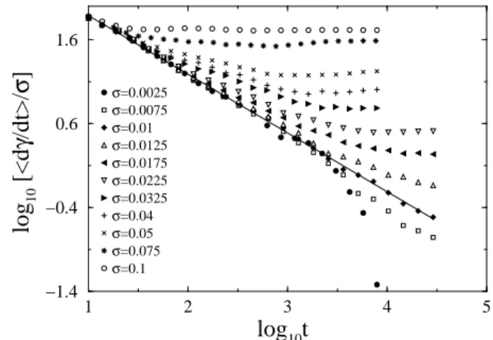
a single slip system under the action of constant stress was shown to give rise to Andrade-like creep at short and in-termediate times for a wide range of applied stresses, with-out invoking thermally activated processes, i.e. T = 0(see Fig. 6). The strain rate, which is proportional to the density of mobile dislocationsdγ/dt=P
ibiviwithvithe velocity of each dislocation, decays as a power law with an exponent close to2/3, in agreement with Andrade’s observations. At larger times, the strain-rate was observed to cross over to a linear creep regime (i.e. to a plateau signaling a steady rate of deformation) whenever the applied stress is larger than a critical thresholdσc, or, otherwise, to decay exponentially to zero.
1 2 3 4 5
log
10t
−1.4 −0.4 0.6 1.6
log
10
[<d
γ
/dt>/
σ
]
σ=0.0025
σ=0.0075
σ=0.01
σ=0.0125
σ=0.0175
σ=0.0225
σ=0.0325
σ=0.04
σ=0.05
σ=0.075
σ=0.1
Figure 6. The strain rate relaxation for different applied stresses at T = 0for a system of sizeL= 100b. The initial density of edge dislocations is around1%. The solid line is the best linear fit of the σ= 0.01curve and yieldsdγ/dt∼t−0.69.
These results suggested that a possible interpretation of dislocation motion and the corresponding creep laws of crystalline materials could also be found within the general “jamming” framework proposed to encompass the wide va-riety of non-equilibrium soft and glassy materials discussed previously. When jammed, these systems are unable to ex-plore phase space, but they can be unjammed by changing the stress, the density, or the temperature. The analogies of dislocation motion and these so-called jammed systems was further explored by considering the influences of dislocation multiplication, and thermal-like fluctuations on the dynam-ics. Dislocation multiplication favors the rearrangements of the system and induces a linear creep regime (flowing phase) at lower stress values, but it does not affect the initial power-law creep. The introduction of a finite effective temperature
101 102 103 104 105
t
10−5
10−4
10−3
10−2
10−1
<v
2 >
1/2
Figure 7. The time evolution of the root-mean-square velocity of four individual runs of the numerical simulations for different ini-tial conditions. The applied stress value in all cases isσ= 0.0075. The curves are depicted in a double logarithmic scale to empha-size the intermittent bursts characteristic of the creep dislocation dynamics around the yield threshold.
The detailed analysis of the model data unveiled the dislocation microscopic dynamics in the Andrade, and in the stationary regimes: Most dislocations are arranged into metastable structures so that the stress field they generate in the material is screened out on large length-scales. These structures consist of small-angle dislocation boundaries sep-arating slightly misoriented crystalline blocks or far more complex dislocation arrangements. If the applied stress is below the yield threshold, dislocations are not able to eas-ily explore the space of configurations to find the most fa-vorable spatial arrangement and they are, most of the time, trapped in metastable configurations which induce a jam-ming of the system. Around the yield threshold, a small fraction of dislocations may, however, attain a higher mo-bility and provoke several intermittent rearrangements of the whole system in the course of time. The stress field generated by these unsettled dislocations conserves the ini-tial long-range character, and forces the system to continue evolving in time in a cooperative manner to try to reduce the internal shear stress (or minimize the elastic energy) by exploring further more favorable arrangements.
In Fig. 7, we show the root-mean-square velocity hv2i1/2(t) = [P
iv2i/N]1/2 of all the dislocations (N ∼ 100−150) present in a square cell of sizeL = 100b as a function of time for four single runs of the numerical sim-ulations. Thus, each run represents the creep behavior of a small piece (a few nanometers big) of a macroscopic system, and starts from a different initial dislocation configuration, obtained after letting the system relax in the absence of ex-ternal load during a given time interval. The exex-ternal shear stress applied is in all casesσ= 0.0075, that is, in the vicin-ity of the critical thresholdσc. We can clearly appreciate the presence of a few intermittent burst after which hv2i1/2(t)
slowly decreases in time. Similar burst, but either positive or negative, can also be observed in the corresponding strain-rate curvesdγ/dt(not shown). Andrade’s power law creep appears as a result of the averaging process over many of these runs, mimicking the behavior of a much bigger sys-tem. The closer is the applied stress to the threshold the
longer is the collective power-law motion before the system falls either in the jammed or in the moving state. Precisely at the critical point and for the case of an infinite system, the Andrade power-law could in principle last indefinitely. C. Non-linear rheology
Above the stress threshold, the system eventually ex-hibits a linear creep regime in which the dislocations present in the system tend to glide in a coherent manner. The depen-dence of the steady strain-rate value on the external shear stress is shown in Fig. 8. Within the error bars, the simu-lation data for the higher stress values considered can be fit quite nicely by a cubic law dependence (see the solid line in the plot). This is an interesting result since, if we were to compare with the nonlinear rheology characteristic of amorphous polymeric networks or other soft glassy materi-als [106], it would correspond to an effective shear-thinning
viscosity for the dislocation ensemble which decreases with
the strain-rate asη = σ(dγ/dt)−1 ∼ (dγ/dt)−2/3. This
result is in good agreement with the theoretical results ob-tained in Ref. [106] and compatible with the power law shear-thinning behaviorη ∼ γ˙−α withα = 0.5−1.0 ob-served in many different complex fluids [7].
10−2 10−1
σ
10−3 10−2 10−1 100 101
d
γ
/dt
~σ3
Figure 8. The steady strain rate value for different applied stresses in a double logarithmic scale. The solid line represents a cubic de-pendence of the formdγ/dt ∼ σ
3
which appears to be in good correspondence with the simulation data for the higher stress val-ues considered.
VI
Conclusions
In this paper we have discussed the collective dynamics of an assembly of interacting particles and, in particular, the transition from a blocked to a moving phase. Transitions of this kind are observed in different contexts and are due to different mechanisms. When the particles are blocked by quenched disorder, one typically refers to the depinning transition, which can be elastic when the medium preserves its topology through the transition, or plastic when topolog-ical defects, such as dislocations, are generated during the dynamics. The driving force for depinning can be due to an externally applied field, or could be self-generated by a den-sity gradient, as in the case of front propagation. When the motion is not hindered by quenched disorder, but by intrinsic constraints one usually refers to a jamming transition.
Common features of depinning and jamming phenom-ena are, at the macroscopic level, the observation of a non-trivial steady-state force-velocity curve, scaling typically as
v∼(F−Fc)βforF > F
c, and a transient power law relax-ation of the velocityv∼t−α. At the microscopic level, pin-ning and jamming systems are both characterized by a com-plex energy landscape, with many metastable states. This leads to an intermittent avalanche-like response to exter-nal perturbations. Thus despite the different origins, pin-ning and jamming have several properties in common which could be possibly used to construct a comprehensive theory of deblocking transitions. Numerical simulations of inter-acting particles have played a major role so far to elucidate the detailed nature of some of these phenomena. The ad-vancement of theoretical understanding is needed to redi-rect numerical simulations from a purely descriptive point of view to a deeper level of analysis.
Acknowledgements
We thank A. A. Moreira, J. Mendes-Filho, A. Vespig-nani and M. Zaiser, who have contributed to the work viewed here. We thank H. F. da Silva for the numerical re-sults reported in Fig. 4. This work is supported by an Italy-Spain Integrated Action. MCM is supported by the Minis-terio de Ciencia y Tecnolog´ıa (Spain). JSA is supported by CNPq. SZ acknowledges FUNCAP for supporting his visit to the Universidade Federal do Cear´a.
References
[1] C. Murray, C. Kagan, and M. Bawendi, Ann. Rev. Mat. Sci.
30, 545 (2000).
[2] T. B. Mitchell, J. J. Bollinger, W. M. Itano, and D. H. E. Du-bin, Phys. Rev. Lett. 87, art n. 183001 (2001).
[3] A. Pertsinidis and X. S. Ling, Nature (London) 413, 404 (2001).
[4] J. Marro and R. Dickman, Nonequilibrium Phase Transitions in Lattice Models (Cambridge University Press, Cambridge, 1999).
[5] H. Hinrichsen, Braz. J. Phys. 30, 69 (2000); J. F. F. Mendes, Braz. J. Phys. 30, 105 (2000); H. Park and S. Kwon, Braz. J. Phys. 30, 133 (2000).
[6] D. Rapaport, The Art of Molecular Dynamics Simulation (Cambridge University Press, Cambridge, 1995).
[7] R.G. Larson, The structure and rheology of complex fluids, (Oxford University Press, New York, 1999).
[8] J.F. Brady and G. Bossis, Annu. Rev. Fluid Mech. 20, 111 (1988).
[9] Y. Yamane, Y. Kaneda, and M. Doi, J. Non-Newtonian Fluid Mech. 54, 405 (1994).
[10] T. Ohta, H. Nozaki, and M. Doi, J. Chem. Phys. 93, 2664 (1990).
[11] S.A. Kahn and R.C. Armstrong, J. Non-Newtonian Fluid Mech. 22, 1 (1986).
[12] J.P. Hirth and J. Lothe, Theory of Dislocations (Krieger Pub-lishing Company, 1992).
[13] M. Kardar, G. Parisi, and Y.-C Zhang, Phys. Rev. Lett. 56, 889 (1986).
[14] A.-L. Barab´asi and H. E. Stanley, Fractals Concepts in Surface Growth, (Cambridge University Press, Cambridge, 1995).
[15] T. Halpin Healy and Y.-C Zhang, Phys. Rep. 254, 215 (1995).
[16] S. He, G. L. M. K. S. Kahanda, and P-Z. Wong, Phys. Rev. Lett. 69, 3731 (1992).
[17] M. A. Rubio, C. A. Edwards, A. Dougherty, and J. P. Gollub, Phys. Rev. Lett. 63, 1685 (1989).
[18] J. P. Stokes, A. P. Kushnick, and M. O. Robbins, Phys. Rev. Lett. 60, 1386 (1988).
[19] M. Dube, M. Rost and M. Alava, Eur. Phys. J. B 15, 691 (2000).
[20] J. Zhang, Y.-C., Zhang, P. Alstrom, and M. T. Levinsen, Phys-ica A 189, 383 (1992).
[21] J. Maunuksela, M. Myllys, O.-P. Kahkonen, J. Timonen, N. Provatas, M.J. Alava and T. Ala-Nissila, Phys. Rev. Lett. 79, 1515 (1997).
[22] A. Br´u, J.M. Pastor, I. Fernaud, I. Br ´u, S. Melle, and C. Berenguer, Phys. Rev. Lett. 81, 4008 (1998).
[23] J. S. Andrade Jr., D. Street, Y. Shibusa, S. Havlin, and H. E. Stanley, Phys Rev. E 55, 772 (1997).
[24] M. Sahimi, Flow and Transport in Porous Media and Frac-tured Rock (VCH, Boston, 1995).
[25] S. Havlin and D. Ben-Avraham, Adv. Phys. 36, 695 (1987).
[26] S. Havlin and A. Bunde, “Percolation II: Transport in Perco-lation Clusters” in Fractals and Disordered Systems, Second Edition edited by A. Bunde and S. Havlin (Springer-Verlag, Berlin, 1996).
[27] E. H. Brandt, Rep. Prog. Phys. 58, 1465 (1995).
[28] G. Blatter, M.V. Feigel’man, V.B. Geshkenbein, A.I. Larkin, and V.M. Vinokur, Rev. Mod. Phys. 66, 1125 (1994).
[29] C. P. Bean, Rev. Mod. Phys. 36, 31 (1964).
[30] Y. B. Kim, C. F. Hempstead and A. R. Strnad, Phys. Rev. 129, 528 (1963).
[31] S. Field, J. Witt, F. Nori, and X. Ling, Phys. Rev. Lett. 74, 1206 (1995); C. M. Argenter, Phys. Rev. B 58, 1438 (1998); K. Behnia, C. Capan, D. Mailly and B. Etienne, Phys. Rev. B
![Figure 1. In the upper panel we show a typical realization of a flux front obtained from a simulation of interacting vortices in a disordered landscape [46]](https://thumb-eu.123doks.com/thumbv2/123dok_br/18979905.456652/5.892.214.709.88.547/figure-realization-obtained-simulation-interacting-vortices-disordered-landscape.webp)