Lat. Am. j. solids struct. vol.12 número2

(1)

Abstract

Interfacial behavior between soil and shallow foundation has been found so influential to combined soil-footing performance and redistribution of forces in the superstructure. This study introduc-es a new thin-layer interface element formulated within the con-text of finite element method to idealize interfacial behavior of soil-framed structure interaction with new combination of degrees of freedom at top and bottom sides of the interface element, com-patible with both isoparametric beam and quadrilateral element. This research also tends to conduct a parametric study on respec-tive parameters of the new joint element. Presence of interface element showed considerable changes in the performance of the framed structure under quasi-static loading.

Keywords

Interface Element; Framed Structure; Interaction Analysis; Finite Element Method

Soil-Framed Structure Interaction Analysis

–

A New Interface Element

1 INTRODUCTION

Presence of interface elements in the context of finite element method has shown significant effect on resultant forces and stresses in the body of structures and has subsequently led to idealization modifications in numerical simulation of interfacial behaviors. Presence of interface element is a necessary need in order to come up with the practical and real nature of behavior of structures sub-jected to lateral load (unsymmetrical system). Different types of joint elements have been intro-duced and formulated for various applications wherever interfacial behavior has been in concern. Interaction of soil and foundation is one of the related topics which has been noticed and of course studied to some extent. As a matter of fact, consideration of such idealization is based on the prac-tical observations that proved the presence of a thin layer of soil right beneath the footing acting unlike the rest of the soil body, (Desai and Rigby, 1995).

M. Dalili Shoaei a Huat B.B.K b M.S. Jaafar c* A. Alkarni d

a,b,c _{Civil Engineering Department,} Fac-ulty of Engineering, University Putra Malaysia, Malaysia

d _{College of Engineering,}_Geotechnical Engineering Faculty, King Saud Universi-ty, Riyadh, Saudi Arabia

* msj@upm.my

http://dx.doi.org/10.1590/1679-78251130

(2)

Latin A m erican Journal of Solids and Structures 12 (2015) 226-249 Other soil-structure interaction model is Winkler model, through which, soil is presented by closely spaced springs. Winkler foundation model is found as a straightforward solution for interac-tion of foundainterac-tion and underlying soil, (Colasanti and Horvath, 2010). Mazzoni and Sinclair (2013) used program OpenSees for nonlinear analysis of an existing building. The foundation was simulat-ed by Winkler model and dashpot, however, shear deformation of soil was neglectsimulat-ed.Soil is a con-tinuum material and continuity of the soil structure corresponds to transverse shear stress which is neglected by Winkler model because of the presence of independent springs. Due to the nature of independent springs, displacement discontinuity occurs between the loaded part and unloaded area of sub-grade soil, i.e. there is no cohesive bond among soil particles. Moreover, behavior of soil is idealized only with sub-grade modulus and none of the key mechanical soil parameters are included. Interface elements in a general categorization have been grouped into two major types generally known as nodal interfaces, e.g. Zero-thickness element, and continuum elements, e.g. thin-layer interface element, Wang and Wang (2006). A review of various joint elements has been carried out by Dalili S. et al. (2013).

Desai et al. (1984) used isoparametric eight-nodded finite element for interface element with uncoupled normal and shear stiffness and applicable to structural and geological interfaces. Para-metric study was conducted in order to get the optimum thickness/width ratio. The best range for thickness/width ratio was found to be 0.01 to 0.1. Hu and Pu (2004) discussed the interface thick-ness to be as thick as five times of the mean sand particle size, i.e. 5D50. An axisymmetric interface

element was formulated by Yuan and Chua (1992) for soil-circular foundations interaction.

Viladkar et al. (1994) presented an isoparametric zero-thickness interface element to investigate the interface characteristics of the soil medium and foundation beam element. It should be noted that the formulated element is numerically compatible with three-nodded beam bending element, representing foundation, with three DOF and considered eight-nodded plane-strain element to mod-el the soil mass with two degrees of freedom per node. Similar interface mod-element was also employed by Noorzaei et al. (1994). In contrast to Desai et al. (1984), Sharma and Desai (1992) and Viladkar et al. (1994) in a study conducted by Mayer and Gaul (2007) zero thickness element was found more suitable for solid-to-solid contact since it has no interfacial thickness, therefore, contact stiff-ness is not dependent of element thickstiff-ness.

Noorzaei et al. (1993) and Viladkar et al. (1994) found Variation of normal stiffness so influen-tial on the general behavior of superstructure since higher values yield less structural sway and low-er values change the behavior of structure to more realistic one. By and large, presence of intlow-erface element caused redistribution of shear stress in footing as well as higher amount of sway, 1.3 times more, compared to the case excluding this type of element. In a comparison conducted by Swamy et al. (2011) between an interactive soil space-framed structure and non-interactive analysis, inter-face modeling was suggested wherever pressures and settlements, i.e., soil settlement and differential settlement, are to be studied.

(3)

Latin A m erican Journal of Solids and Struc tures 12 (2015) 226-249

on homogeneous single-layered soil was subjected to quasi-static inclined and eccentric load. Sheng and his fellow researchers concluded that smoothness of the footing-soil contact is a key parameter to bearing capacity of soils with self-weight.

In this paper a new interface element has been formulated to idealize interfacial behavior be-tween the underlying soil and shallow footing, e.g. strip and pad/raft ones, supporting plane-framed superstructure. The new interface element is of the thin-layer type and suitable for soil continuum-footing-superstructure interaction analysis. Based on the literature carried out, it was found that all the related types of interface developed for soil-structure interaction are not actually fully compati-ble with the beam element employed for infrastructure simulation. Bearing in mind that the previ-ously employed three-node beam bending element as well as the latest two-node beam element have three degrees of freedom per node (u, ν, θ), consider 2D analysis, two translation and one rotation while the rotation has never been considered as a degree of freedom in the joint element formulation whose effect on the superstructure is to be studied in the present paper in addition to other related substantial features. Presence of the developed interface element has shown considerable variation and redistribution of forces in the superstructure under quasi-static loading such that elements may subject to section modification.

2 MATHEMATICAL FORMULATION

2.1Two-nodded Isoparametric Beam and Eight-node Serendipity Elements

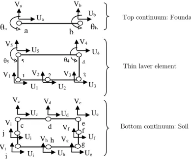
For straight prismatic beam member employed herein for superstructure and infrastructure idealiza-tion, Figure 1, it is assumed that the displacements are small enough so that secondary effects like beam shortening as a consequence of bending are ignored. Complete formulation of considered beam element stiffness matrix has been carried out elsewhere by Coates et al. (1988) in explicit form which has been used for the current study.

Figure 1:Thin-Layer Element Located Between Two Finite Elements. Top continuum: Foundation

Thin layer element

Bottom continuum: Soil

Uc Ud Ue

Uj Uf

Ui Uh Ug

Vc Vd Ve

Vj

Vi

Vh Vg Vf

c _d e

f

g h

i j

U1 U2 U3

1 2 3

V1 V2 V3

5 θ4 ₄

θ5

U4 U5

V4 V5

Ua Va

a

Vb Ub

θ

b

θ

a

(4)

Latin A m erican Journal of Solids and Structures 12 (2015) 226-249 The selected eight nodded quadrilateral element, Figure 1, from serendipity family of finite elements is the most well-known one, utilized for soil simulation in earlier research works under plane strain condition. Many researchers have used this element for soil and solid material modeling in geotech-nical and soil-structure interaction analyses like Noorzaei et al. (1995), Karabatakis and Hatzigogos (2002), Sheng et al. (2007) and Agrawal and Hora (2010). This element with two degrees of freedom per node can suitably idealize the translational moves of the soil body whose stiffness matrix is gen-erated within the program in conventional way.

Despite the simplicity of a mapped meshing and straightforward numerical implementation of eight nodded quadrilateral element, based on which, it was selected for the current study, similar analyses which regarded coupled soil-foundation system also discussed the convergence rate and computational efficiency of other meshing techniques. Foye et al. (2008) and Teodoru (2009) used triangular element which can be utilized for free unstructured meshing by available commercial finite element-based software. Unstructured mesh permits rapid transition in mesh density and therefore, an illustrative rate of convergence can be provided. Due to the well-shaped geometry of quadrilateral finite elements, they cannot be employed for free meshing technique. Jahromi et al. (2009) employed partitioning technique for idealization of a large-scale soil medium as a part of coupled soil-structure model.

2.2 Five-node Isoparametric Interface Element

The newly developed interface element has five nodes connecting the beam element with three de-grees of freedom per node to the soil element with two dede-grees of freedom per node. Therefore, the thin-layer interface element has three degrees of freedom per node associated with upper side nodes and two degrees of freedom associated with translational degrees of freedom of the underlying soil element to discretize the thin-layer interfacial behavior between soil and infrastructure, Figure 1. The detail formulation of this element which leads to generation of its stiffness matrix in explicit form is presented hereafter.

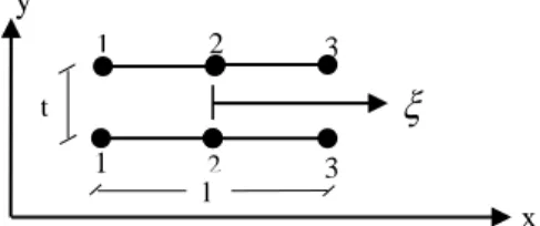
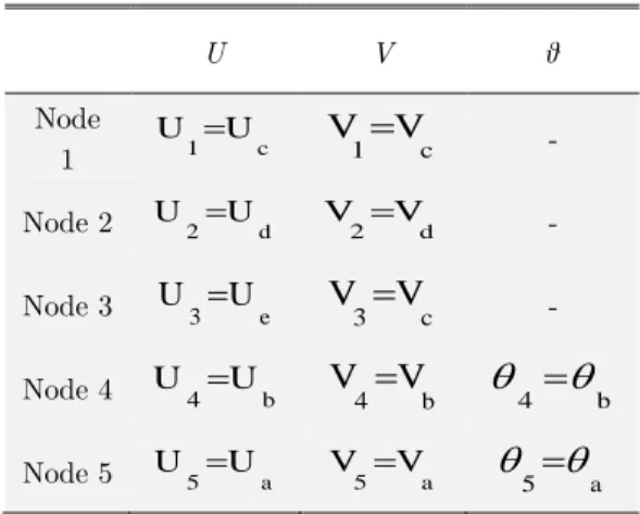
As depicted in Figure 2, Formulation of the thin-layer interface element begins by assembling two one-dimensional three-nodded elements from isoparametric element families located at the thin distance of t. However, due to the incompatibility with the top two-nodded beam element that orig-inates by presence of the middle node at the upper side of the interface element, not depicted in Figure 1, this node is eliminated. Therefore, displacements of nodes 1 to 5 in Figure 1 can be ex-pressed as presented in Table 1 while associated displacements of the eliminated node are calculated as the average values of adjacent upper nodes (nodes a and b) by equations (1.a) to (1.c). These expressions are then implemented in the intermediate transfer matrix.

Figure 2:Thin-layer element with two three-nodded elements at top and bottom. 2

2 y

1 3

t

l

x x

(5)

U V θ

Node

1 U1Uc V1Vc -

Node 2 U2Ud V2Vd -

Node 3 U₃U_e V₃



V_c -

Node 4 U₄U_b V₄



V_b



₄



_b

Node 5 U5Ua V5Va



5



a

Table 1: Displacements of Interface Nodes.

2

*

b

a U

U

U  

(1.a)

2

*

b

a V

V

V   _(1.b)

2

*

b

a



  (1.c)

Notations U, V and



represent horizontal and vertical translations and rotation respectively. Ex-pressions in Table 1 can be written in matrix form depicting how nodal degrees of freedom are con-nected:

1 12 12 15 1

15



[T]  { } 

}

Δ

{

₍₂₎

Where { , , , , , }

5 * 4 3 2

1





}

{

Δ

_and

{

}

{

,

}

a b e d

c





. In equation (2),{Δ} stands for vector of interface element displacements and

{

}

_{is vector of displacement of adjacent elements}

(6)

Latin A m erican Journal of Solids and Structures 12 (2015) 226-249 1 12 12 15 1 15 5 5 5 * * * 4 4 4 3 3 2 2 1 1 1 0 0 0 0 0 0 0 0 0 0 0 0 1 0 0 0 0 0 0 0 0 0 0 0 0 1 0 0 0 0 0 0 0 0 0 5 . 0 0 0 5 . 0 0 0 0 0 0 0 0 0 0 5 . 0 0 0 5 . 0 0 0 0 0 0 0 0 0 0 5 . 0 0 0 5 . 0 0 0 0 0 0 0 0 0 0 1 0 0 0 0 0 0 0 0 0 0 0 0 1 0 0 0 0 0 0 0 0 0 0 0 0 1 0 0 0 0 0 0 0 0 0 0 0 0 1 0 0 0 0 0 0 0 0 0 0 0 0 1 0 0 0 0 0 0 0 0 0 0 0 0 1 0 0 0 0 0 0 0 0 0 0 0 0 1 0 0 0 0 0 0 0 0 0 0 0 0 1 0 0 0 0 0 0 0 0 0 0 0 0 1                                                                                                                                            a a a b b b e e d d c c V U V U V U V U V U V U V U V U V U V U V U    

 (3)

Since the proposed interface element is from isoparametric family, displacements and rotations at any point can be defined conventionally in terms of shape functions, (Viladkar et al., 1994):







n

i i i

U

N

U

1

(4.a)







n

i

N

i

V

i

V

1

(4.b)







n

i i i

N

1



(4.c)

In equation (4), Ni stands for shape functions of nodes 1, 2 and 3 in Figure 2 and they are:

) 1 ( 2 1 1







N

,

(1 2)

2 



N

and

(1 )

2 1 3







N

(5)

(7)

{ [B]{ } [B][T]{ } [BJ]{ }

t Δ t t t V V t U U V U t } top bot top bot top s n s                                           

 ( ) 1 1

) ( 1 2 1







(6)

Strain components_s₁,



_s₂and



_n are representing tangential strain, rotational strain and normal strain associated with the counterpart relative displacements U,  and V respectively. Nota-tions top and bot correspond to the top and bottom of the continuum. The shape function matrix [B ] is, (Viladkar et al., 1994):

















3 2 1 3 2 1 3 2 1 3 2 1 3 2 1 N 0 0 N 0 0 N 0 0 0 0 0 0 0 0 0 N 0 0 N 0 0 N 0 N 0 N 0 N 0 0 0 N 0 0 N 0 0 N 0 N 0 N 0 N [B]

(7)

and [BJ] is strain-displacement matrix.

12 15 15 3 t 1  

 [B] [T]

] [B

J

(8) Based on total potential energy, stiffness matrix is calculated from equation below:

    



1 1 t 0 T v T 12

12

[B

]

[D

][B

]

dv

[B

]

[D

][B

]

(det

J

)

d



d



[k]

J I J J I

J

(9)

Where [DI] is elasticity matrix, Coutinho et al. (2003),

[D] [D] ] [D I _t 1 d t 1 t 0 2 

 



(10)

In equation (9), det J=l/2 since 1-D element was selected from the very beginning (Figure 2). It is noteworthy that in equation (9) elasticity matrix, [DI], is in global form. However, [D ] in equation

(10) is in local form and should be transformed into global one. The local elasticity matrix [D ] is comprised of three uncoupled stiffness components:

             2 s s n n s 1 s k 0 0 0 k 0 0 0 k

[D]

₍₁₁₎

(8)

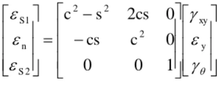
Latin A m erican Journal of Solids and Structures 12 (2015) 226-249 The normal strain ( )

ν and shear strains (s1,s2 ) in the local coordinate system are related to

global strains,



y,



xy and



as:



















































y xy S n S c cs cs s c

1

0

2

2 2 2 2 1

(12)

Where

s



sin



,

c



cos



,





the inclination of the interface to the x-axis (Figure 3) and [Tˆ] is

the transformation matrix of strains from global vector {ε} to local vector

{

}

_.

Stress-strain relationship is presented by:

}

{ ] T [ [D] ] T [

σ}

{d

ˆ

d

g T

g



(13)

Where [Tˆ] was presented in equation (12), [D ]g is the global constitutive matrix and

{

d

σ}

and

}

d

{

_{are global stress and strain vectors. The local constitutive matrix}_{[D ]}_{gets transformed to}

global constitutive matrix [D ]g by equation (14).

Figure 3: Thin-layer element in local and global coordinate systems.

 

























































3 2 4 4 1 2 2 2 2 s s n n s 1 s 2 2 2 g

D

0

0 D

D

0 D

D

1

0

0 c

cs

0 2cs

s

c

k

0

0 k

0

0 k

1

0

0 c

2cs

0 cs

s

c

D

(14)

(9)

Latin A m erican Journal of Solids and Struc tures 12 (2015) 226-249                                                                                         3 2D 0 3 2D 0 3 2D 3 2D 3 D 0 0 3 2D 0 3 D 3 D 0 3 2D sym. 0 3 D 3 D 0 3 2D 3 2D 0 3 D 3 D 0 0 0 15 4D 0 3 D 3 D 0 0 0 15 4D 15 4D 0 3 2D 3 2D 0 3 2D 3 2D 15 2D 15 2D 15 16D 0 3 2D 3 2D 0 3 2D 3 2D 15 2D 15 2D 15 16D 15 16D 0 0 0 0 3 D 3 D 15 D 15 D 15 2D 15 2D 15 4D 0 0 0 0 3 D 3 D 15 D 15 D 15 2D 15 2D 15 4D 15 4D 2t l 3 2 4 1 3 3 2 4 2 4 1 4 4 2 4 2 4 1 4 1 2 4 2 4 2 4 2 4 1 4 1 4 1 4 1 2 4 2 4 2 4 2 4 1 4 1 4 1 4 1 [k]

(15)

2.3Constitutive model for soil

Most of the soils follow a nonlinear constitutive relation. This well established fact has led pioneers to use various stress-strain relationships for soil continuum. Several models have been proposed for soil behavior whose precision evaluation is not within the scope of the current study. However, in order to treat the soil as a nonlinear body, hyperbolic model has been employed to account for the material non-linearity of the soil media. The tangent modulus at any stress level may be expressed as,







n

a a f t P kP c R E























3 2 3 3 1

sin

2 cos

2 sin

1

1 









(16)

This expression for tangent modulus of elasticity can be implemented very conveniently in an in-cremental stress analysis in which Rfrepresents failure ratio,



is angle of internal friction,



1 and

3



stand for major and minor principal stresses respectively, c and k are cohesion and modulus number of the soil. Pa is atmospheric pressure and n is exponent which depicts the variation of

ini-tial tangent modulus

E

iwith respect to minor principal stress. The Poisson's ratio was assumed to

(10)

Latin A m erican Journal of Solids and Structures 12 (2015) 226-249

Param eter D escription M

agni-tude

f

R _{Failure ratio} _0.85



Interface angle of friction () 37.5

C Cohesion (_N_{/ mm}2₎ _0.0

*

k

Modulus number 500

a

P

Atmospheric pressure ₍ _{/ mm}2

N ) 0.10132

*

n

Exponent 0.92

s



Poisson's ratio 0.3

Relative density of the soil was assumed to be 80%.

*_{corresponding to the confining pressure,} 2

310N/cm

 .

Table 2:Soil parameters for nonlinear analysis.

2.4 Evaluation of interface characteristics

There are three stiffness parameters, introduced earlier, associated with stress-strain relationship of the interface element which is simulated by the hyperbolic constitutive model. The current study presents some useful information regarding proper values of stiffness parameters of the developed thin-layer interface element. Two ranges were assigned for the normal (Knn) and rotation (Kss2)

stiffness while tangential stiffness (Kss1) is calculated as, Noorzaei et al. (1994):

i

ss K

K ₁ (1



₂)2

(17) where:

n

a n w j i

P k

K





[



]

(18)

)

tan

(

2









n a

f

c

R





(19)



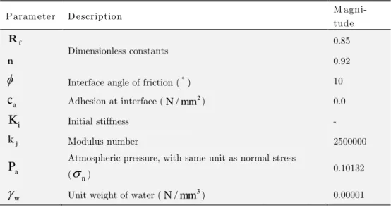
stands for shear stress and other interface element parameters for nonlinear analysis are presented in Table 3, Viladkar et al. (1994) and Desai et al. (1974).

(11)

those recommended in the literature will not work out for the developed interface element in the current research.

Param eter D escription M

agni-tude

f

R

Dimensionless constants 0.85

n 0.92



Interface angle of friction () 10

a

c

Adhesion at interface ( 2

/mm

N ) 0.0

i

K

Initial stiffness -

j

k _{Modulus number} _2500000

a

P

Atmospheric pressure, with same unit as normal stress ₍

n



) 0.10132

w



Unit weight of water ( 3

/mm

N ) 0.00001

Table 3:Parameters for Nonlinear Interface Analysis.

In this investigation, constant magnitudes of Knn and Kss2 have been used throughout the analysis.

Due to absence of similar model in literature, values were worked out on the basis of trial and error analysis looking for the proper ranges with respect to the current frame structure-foundation-soil analysis to avoid unexpected results. Former researchers such as Sharma and Desai (1992) and Vi-ladkar et al. (1994) assigned arbitrary values for stiffness parameters of interface element. Further, Kss2 was found to lie between 106 and 1010 MPa. Three values of 106, 108 and 1010 MPa were chosen

to study the influence of such variation on combined footing-soil performance. Proper range for normal stiffness also varies between 4000 to 10000 MPa and three values were assigned for this parameter as 4000, 7000 and 10000 Mpa. Values beyond the given ranges for Knn and Kss2 were

found either with no effect on the structural performance or they would cause drastic alteration of internal forces which was never anticipated nor reported by former researchers. The following dis-cussion will highlight the influence of the selected values on the overall behavior of the framed structure as well as the supporting soil.

3 COMPUTER IMPLEMENTATION

(12)

Latin A m erican Journal of Solids and Structures 12 (2015) 226-249 the load steps and the residual force, the force difference between applied external force and stresses that have satisfied the constitutive laws, is redistributed on the elements. This redistribution takes as many iterations as needed to meet the convergence criterion prior to the next load step.

4 NUMERICAL EXAMPLE

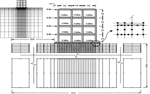
In order to verify the developed model associated with the constitutive law for thin-layer interface element and to investigate its influence on the response of a structure, interactive behavior of a plane-frame four-storey structure together with the combined footing-soil system is studied hereaf-ter. This model is similar to the analysis model presented by Viladkar et al. (1994), where the 2D two-bay five-storey reinforced-concrete frame was supported by a combined soil-footing system and studied under pushover analysis. A three-node isoparametric zero-thickness element was used to present the interface element. Loading, dimensions of structural elements and constitutive laws that govern the soil and interfacial behaviors were also similar to the aforementioned model. Therefore, despite having a few differences to Viladkar's model such as the soil modulus of elasticity and struc-tural geometry, some similarities in the overall performance of the developed thin-layer interface element compared with that of Viladkar's analysis were anticipated and considered as verification of the developed model in the current research.

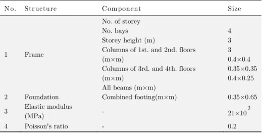
The considered frame was subjected to both vertical and lateral loading, making the current case an unsymmetrical system, as shown in Figure 4. Therefore, differential settlements will be of great importance in addition to the other aspects of the interaction analysis. The selected plain frame was assumed to be a part of a long space frame resting on a raft foundation. There was no variation of vertical and horizontal loading along the longitudinal direction, thus the soil can be treated as in plane strain. Geometrical details as well as material properties of the considered frame are presented in Table 4.

(13)

In a study on the settlement of shallow footing resting on clay, conducted by Foye et al. (2008), it was reported that the mesh density below the footing has larger effect on the nonlinear models compared to boundary distances. Similar result was also reported by Kumar and Kouzer (2007). Therefore, this study used relatively small meshing and a large domain to ensure that the boundary conditions have minimal effect on the resultant forces and stresses as depicted in Figure 4. Depth and width of the supporting soil which was modeled by eight nodded quadrilateral element were 50m and 51m, respectively, where the vertical side boundaries were restrained such that no horizon-tal displacement would occur and the far lower horizonhorizon-tal soil boundary was assigned to be pinned where neither horizontal nor vertical movement was allowed.

The underlying soil was assumed as a layered one so that three different layers were idealized to represent the non-homogeneity of the soil at different depths. Variation of modulus of elasticity along the depth of soil is presented in Table 5. The selected example consisted of 612 soil elements, 52 beam elements and 24 interface elements. It should be mentioned that the thickness of the inter-face was selected as five centimeters which complies with that recommended by Desai et al. (1984),

1 . 0 01 .

0 t l .

N o. Structure Com ponent Size

1 Frame

No. of storey No. bays

Storey height (m)

Columns of 1st. and 2nd. floors (m×m)

Columns of 3rd. and 4th. floors (m×m)

All beams (m×m)

4 3 3 0.4×0.4 0.35×0.35 0.4×0.25

2 Foundation Combined footing(m×m) 0.35×0.65

3 Elastic modulus

(MPa) - 21×10

3

4 Poisson's ratio - 0.2

Table 4: Geometrical details and material properties of the plane frame and combined footing.

Soil layer D epth

(m )

Elastic m odulus (M Pa) 1

2 3

9 21 20

15 45 65

Table 5: geotechnical parameters of the underlying soil.

(14)

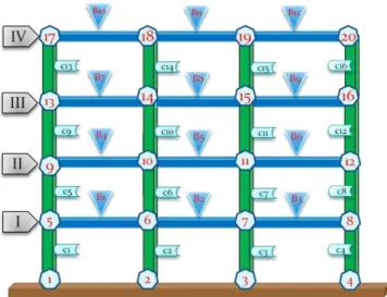
fol-Latin A m erican Journal of Solids and Structures 12 (2015) 226-249 lowing discussion will highlight the effect of the developed interface element on the entire behavior of the structure whose components are labeled as shown in Figure 5.

Case N o.

k

nn(M Pa)

k

ss2(M Pa)

1 4000 106

2 7000 106

3 10000 106

4 7000 108

5 7000 1010

WOINTFC (excludes interface ele-ment)

Table 6: Various cases considered in this study.

Figure 5: Labels of structural elements.

5 RESULT AND DISCUSSION

5.1 Axial forces in columns

(15)

axial force which means choosing high values of this parameter may not lead to any further influ-ence or modification in the axial force of columns.

On the other hand, alteration of Kss2 also demonstrated a similar variation trend for its three

different values. Case 4 and 5 led to average values of 2.97% and 9.75% reduction of axial force of external columns and 2.58% and 8.49% increase in the inner columns with respect to case WOINTFC. This means that case 5 with Kss2 = 1010 N.mm had the largest effect. The reason may

lie in the foundation absorbing greater force, so the expected influence is then amplified. Storey

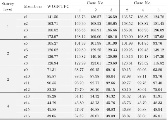
level M em bers W OIN TFC

Case N o. Case N o.

1 2 3 2 4 5

1

c1 141.50 135.73 136.57 136.59 136.57 136.39 124.78

c2 163.71 169.30 168.52 168.65 168.52 168.82 181.45

c3 180.82 186.85 185.91 185.66 185.91 185.93 196.09

c4 173.97 168.12 169.00 169.10 169.00 168.87 157.68

2

c5 105.27 101.39 101.98 101.99 101.98 101.85 93.76

c6 126.02 129.80 129.25 129.33 129.25 129.45 138.12

c7 136.77 140.82 140.16 139.99 140.16 140.18 147.30

c8 126.94 122.99 123.61 123.69 123.61 123.52 115.82

3

c9 71.31 68.77 69.15 69.16 69.15 69.06 63.80

c10 85.87 88.33 87.98 88.04 87.98 88.11 93.76

c11 90.55 93.20 92.77 92.66 92.77 92.78 97.40

c12 82.28 79.70 80.10 80.15 80.10 80.04 75.04

4

c13 35.28 34.15 34.32 34.32 34.32 34.28 31.91

c14 44.79 45.89 45.73 45.76 45.73 45.79 48.33

c15 45.88 47.07 46.88 46.83 46.88 46.88 48.94

c16 39.05 37.89 38.07 38.09 38.07 38.05 35.81

Table 7:Variation of axial force (kN) in columns for various values of Knn and Kss2 and for the case without interface element.

5.2 Shear forces at columns

Table 8 depicts variation of shear forces at the lower joint of every column. It is clear that utiliza-tion of the interface element has reduced column shear forces to some extent while such alterautiliza-tion changed slightly against increasing normal stiffness. Shear forces associated with columns at level one were subjected to degradation for all cases with average percentage of 20.24%, 17.7% and 17.49% for cases 1 to 3, respectively, compared to case WOINTFC. However, this trend did not repeat for higher storey levels. Some of the columns also faced slight increase of shear forces. Hence, variation of shear force along the storey levels did not follow a similar pattern. Cases 4 and 5 also resembled the alteration pattern of other cases with respective magnitudes of 18% and 54%. This shows that case 5 had higher impact on the resultant shear forces of the first storey level.

(16)

Latin A m erican Journal of Solids and Structures 12 (2015) 226-249 According to Table 9, redistribution and reduction of moments were considerable in columns com-pared to the case without interface element. These changes were higher at the first storey level where the inner and outer columns experienced diminishing moment redistribution compared to case WOINTFC. Presence of the interface element in cases 1 to 3 had diminished column moments throughout the frame by an average of 16%, 13.75% and 13.56% respectively. However, some other columns at upper storey levels had been subjected to marginally higher values of moments than those of case WOINTFC.

Storey

level M em bers W OIN TFC

Case N o. Case N o.

1 2 3 2 4 5

1

c1 -27.67 -18.49

-19.11 -18.87

-19.11

-18.87 -7.06

c2 -7.63 -5.95 -6.35 -6.50 -6.35 -6.37 -1.92

c3 30.55 29.19 29.53 29.45 29.53 29.36 22.95

c4 44.75 35.25 35.93 35.91 35.93 35.87 26.03

2

c5 -5.18 -5.78 -5.85 -5.90 -5.85 -5.86 -5.49

c6 8.78 9.82 9.70 9.71 9.70 9.73 11.36

c7 11.18 10.10 10.22 10.23 10.22 10.21 8.81

c8 15.22 15.86 15.93 15.96 15.93 15.92 15.32

3

c9 -7.36 -6.36 -6.49 -6.49 -6.49 -6.46 -4.63

c10 3.03 3.74 3.62 3.60 3.62 3.63 5.09

c11 9.83 9.16 9.27 9.27 9.27 9.24 7.64

c12 14.49 13.47 13.61 13.62 13.61 13.59 11.90

4

c13 -17.10 -15.84 -16.03 -16.04 -16.03

-15.99 -13.34

c14 -0.26 0.94 0.75 0.73 0.75 0.78 3.06

c15 7.55 6.38 6.55 6.56 6.55 6.51 4.10

c16 19.81 18.53 18.73 18.76 18.73 18.70 16.18

Table 8:Variation of shear force (kN) in columns for various values

Knn and Kss2 and for the case without interface element.

A similar trend can be identified for case 4 and 5 but changes associated with case 5 were found to be much greater. Case 4 has degraded the moments associated with columns by an average of 14.4% while case 5 has caused reduction of column moments by 34.78%. It is worth mentioning that the discussed pattern of alteration for column moments is somewhat different to what is reported in literature. Although changes at the first storey were reported to be greater compared to other lev-els, which was expected, variation of resultant moments for different considered cases (case 1 to case 4) barely differed from each other. Rise of normal stiffness in cases 1 to 3 did not impact the mo-ment redistribution in a subtractive trend which has been reported in literature. Furthermore, none of the columns suffered any reversal of moment in this example except case 5 at level 4 (column c14).

(17)

Variation and redistribution of moments are depicted in Table 10. It is clear that alteration of beam moments corresponding to the presence of interface element was more apparent at the outer bays along the height of the structure compared to the inner bay. Increase of normal stiffness has led to small variation of moments while degradation of moments was obvious after applying the interface element. In cases 1 to 3, beam moments were attenuated through the whole considered frame by 13.66%, 10.84% and 11.5%, respectively.

Furthermore, it was found that at higher values of normal stiffness, moments associated with the outer bays of the two lower storey levels also increased slightly while it was the reverse for the inner bay. This trend was not found for the two upper levels where rise of normal stiffness led to gradual growth of all moments, which were still lower than case WOINTFC excluding some of the beams which encountered increase of moment. Increase of rotational stiffness as depicted in Table 10 (con-sider cases 2 and 4) led to marginal degradation of moments. Case 4 caused 11.8% reduction of beam moment while values corresponding to the peak value of Kss2 (case 5) resulted in the largest

reduction of beam moment of 40.23% compared to the case with no interface element.

Storey

level m em bers Ends W OIN TFC

Case N o. Case N o.

1 2 3 2 4 5

1

c1 1

5

-52.85 -30.17

-32.06 -23.40

-33.40 -23.92

-32.81 -23.80

-33.40 -32.83 -6.16 -23.92 -23.76 -15.02

c2 2 -15.38 -12.40 -13.21 -13.51 -13.21 -13.23 -4.06

6 -7.52 -5.44 -5.85 -6.00 -5.85 -5.87 -1.70

c3 3 66.83 64.46 65.13 65.00 65.13 64.81 51.90

7 24.83 23.11 23.44 23.36 23.44 23.28 16.95

c4 4

8

97.14 37.11

75.54 30.20

77.04 30.75

77.01 30.73

77.04 76.94 55.43 30.75 30.68 22.66

2

c5 5

9

-1.99 -13.56

-4.72 -12.63

-4.72 -12.84

-4.84 -12.87

-4.72 -4.76 -6.24 -12.84 -12.81 -10.22

c6 6 15.77 17.23 17.11 17.15 17.11 17.17 19.17

10 10.57 12.23 12.00 11.98 12.00 12.03 14.91

c7 7 13.84 12.24 12.38 12.42 12.38 12.39 11.21

11 19.71 18.06 18.28 18.28 18.28 18.23 15.22

c8 8

12

17.07 28.60

19.91 27.68

19.89 27.90

19.95 27.93

19.89 19.89 20.79 27.90 27.86 25.15

3

c9 9

13

-13.48 -8.59

-11.79

-7.30 -11.99 -7.48

-11.97

-7.49 -11.99

-11.94 -8.96 -7.48 -7.44 -4.93

c10 10 2.68 3.69 3.51 3.47 3.51 3.53 5.72

14 6.42 7.53 7.35 7.32 7.35 7.37 9.55

c11 11 13.08 12.11 12.28 12.28 12.28 12.24 9.82

15 16.42 15.36 15.52 15.52 15.52 15.48 13.11

c12 12

16

20.32 23.14

18.58 21.83

18.80 22.02

18.82 22.04

(18)

Latin A m erican Journal of Solids and Structures 12 (2015) 226-249 4

c13 13

17

-22.75 -28.55

-21.21 -26.31

-21.45 -26.65

-21.46 -26.66

-21.45 -21.40 -18.11 -26.65 -26.57 -21.92

c14 14 -1.67 -0.09 -0.33 -0.36 -0.33 -0.29 2.70

18 0.89 2.89 2.58 2.54 2.58 2.62 6.48

c15 15 9.05 7.49 7.72 7.73 7.72 7.67 4.53

19 13.60 11.64 11.94 11.94 11.94 11.87 7.79

c16 16 23.02 21.46 21.71 21.74 21.71 21.67 18.53

20 36.40 34.12 34.48 34.52 34.48 34.43 30.00

Table 9:Variation of column moments (kN.m) for different cases.

5.5 Moment of foundation beam

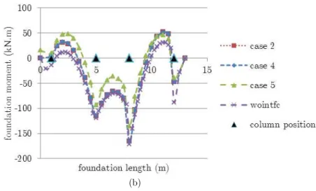
Variation of normal and rotational stiffness has impacted the foundation moment and the results are presented in Figure 6. Generally speaking, the overall trend of foundation moment along the footing has remained the same where results associated with cases 1 to 3 (Figure 6(a)) showed larg-er effect on the portion of the footing supporting the outlarg-er bays such that the curve has been pushed upward compared to case WOINTFC. Similar behavior can be seen for cases 4 and 5 where in case 5 the curve has been entirely shifted upward without any further deviation as far as the peak values of foundation moment are concerned, as shown in Figure 6(b).

Storey

level m em bers Ends W OIN TFC

Case N o. Case N o.

1 2 3 2 4 5

1

B1 1

5

32.15 28.13 28.64 28.64 28.64 28.53 21.25

-7.24

-10.76

-10.26 -10.24 -10.26 -10.36 -17.18

B2 2 -1.02 -1.04 -1.00 -0.92 -1.00 -0.94 -0.28

6 -24.74 -24.94 -24.91 -24.83 -24.91 -24.84 -24.17

B3 3 -13.93 -10.40 -10.92 _10.96- -10.92 -10.83 -3.99

7 -54.18

-50.11

-50.65 -50.69 -50.65 -50.56 -43.46

2

B4 5

9

27.04 24.42 24.83 24.85 24.83 24.74 19.18

-11.19 -13.93 -13.52 -13.51 -13.52 -13.61 -19.31

B5 6 -2.06 -1.99 -1.99 -1.94 -1.99 -1.95 -1.32

10 -23.08 -23.25 -23.21 -23.16 -23.21 -23.18 -23.20

B6 7 -9.71 -6.91 -7.35 -7.41 -7.35 -7.29 -1.84

11 -48.92 -46.27 -46.70 -46.75 -46.70 -46.63 -41.24

3

B7 9

13

31.33 28.51 28.94 28.95 28.94 28.84 23.04

-7.25 -10.04 -9.62 -9.61 -9.62 -9.72

-15.51

B8 10 2.49 2.60 2.60 2.65 2.60 2.64 3.27

14 -18.69

-18.91 -18.87

-18.82

-18.87

-18.83 -18.83

B9 11 -6.78 -3.94 -4.38 -4.43 -4.38 -4.32 1.20

15 -46.16 -43.29 -43.73 -43.78 -43.73 -43.67 -38.13

4 B10 13

17

28.55 26.31 26.65 26.66 26.65 26.57 21.92

(19)

B11 14 6.53 6.82 6.79 6.83 6.79 6.83 7.78

18 -13.82 -14.21 -14.14 -14.09 -14.14

-14.11

-14.54

B12 15 0.22 2.57 2.20 2.15 2.20 2.25 6.76

19 -36.40 -34.12 -34.48 -34.52 -34.48 -34.43 -30.00

Table 10:Variation of beam moments (kN.m) for different cases.

5.6 Settlement and sway

Presence of the interface has led the settlement to be considerably larger than the case without interface element. According to the results presented in Figure 7(a), the larger the normal stiffness, the lesser the foundation settlement is, where a thoroughly different settlement trend is achieved from cases 1 to 3. The largest differential settlement happened for case 1 which was half as large as case WOINTFC, whose normal stiffness was less than the other two cases and showed a steady downward trend while cases 2 and 3 displayed a rapid decline until the center line of the structure and thereafter the downward trend slowed down. Maximum settlement was found at the right end of the footing for cases depicted in Figure 7(a). Differential settlements associated with increment of rotational stiffness showed a different trend compared to former cases, as presented in Figure 7(b). Although the settlement trend in case 4 resembled that of case 2, the increment of rotational stiff-ness (case 5) changed this trend to a great extent. Case 5 resulted in a steady fall of settlement up to the centerline of the frame after which a marked rise was found. This means that the inner bay suffered larger displacements compared with outer ones which resulted in a greater degree of force redistribution in the frame elements.

(20)

Latin A m erican Journal of Solids and Structures 12 (2015) 226-249 (b)

Figure 6: Foundation moment (a) cases 1 to 3 (b) cases 2, 4 and 5.

Application of interface element certainly causes shifting of the whole structure in the direction of the horizontal force while considered cases, as shown in Figure 8, reveal slight differences corre-sponding to the assigned values for interface element parameters. In accordance with Figure 8, low-er normal stiffness causes more shifting of the frame, such as in case 1. Cases 2 to 4 depicted a simi-lar trend of sway for the left end column of the frame. Most strikingly among the considered cases, the last one presents quite a different horizontal displacement curve for storey levels and therefore it shows the way higher rotational stiffness of the footing affects the overall behavior of the super-structure against the external horizontal force.

(21)

Latin A m erican Journal of Solids and Struc tures 12 (2015) 226-249 (b)

Figure 7: Foundation settlement (a) cases 1 to 3 (b) cases 2, 4 and 5.

Figure 8:Variation of sway of the frame along the height.

5.7 Soil compression stress

(22)

Latin A m erican Journal of Solids and Structures 12 (2015) 226-249

(a) (b)

(c)

Figure 9:Normal stress contours in the soil body (MPa) (a) Case WOINTFC (b) Case 1 (c) Case 5.

According to Figures 9(a) to 9(c), application of the interface element resulted in the contours being distributed more smoothly along 50 meters of soil depth while case WOINTFC led to a very differ-ent appearance of stress contours. On the other hand, Figures 9(b) and 9(c) demonstrated a conical distribution of normal stress which continued into the deep layer of the soil so that the deeper layer experienced higher normal stress compared to case WOINTFC. Increase of rotational stiffness has slightly changed the stress distribution that has been induced in both the first few meters and deep in the soil.

6 CONCLUSION

(23)

the presence and absence of the developed interface element. This technique was then codified in a finite element program in FORTRAN environment. Various aspects of such interaction were cov-ered and discussed to investigate the performance of the interface thin-layer element and their cor-responding effects on the superstructure. The shear stiffness was assigned to be a function of normal pressure while the normal and rotational stiffness were set to vary between the optimal range of 4000 MPa to 10000 MPa and 106 to 1010 MPa, respectively. The optimum range for thickness of the interface element can be suggested as between 5 to 50 millimeters. This analysis employed a thick-ness of 50 millimeters.

In a comparison between results retrieved from literature and those of the current study, there were deviations and similarities when the interface element was put into action. First of all, the thin-layer element parameters that defined its stiffness were found to lie in different ranges com-pared with those available in literature. Furthermore, a degree of freedom was added that joins the rotational stiffness of the interface element to that of the beam element and its influence was stud-ied.

Results showed that the presence of interface layer can considerably change the induced forces and stresses both in the superstructure and in the soil body. Nonetheless, variation of thin-layer element parameters led to changes which seems to be more practical compared to similar studies that reported large differences through alteration of interface element parameters.

Acknowledgments

This research received financial support from Universiti Putra Malaysia and King Saud University, under research project No. 67001. All supports from both universities are gratefully acknowledged.

References

Agrawal R. and Hora M.S. (2010). Effect of differential settlements on nonlinear interaction behaviour of plane frame-soil system.ARPN Journal of Engineering and Applied Sciences, Vol. 5, No. 7, pp. 75-87.

Coates, R.C., Coutie, M.G. and Kong, F.K. (1988). Structural Analysis, Spon Press.

Colasanti, R.J., and Horvath J.S. (2010). Practical subgrade model for improved soil-structure interaction analysis: software implementation.Practice Periodical on Structural Design and Construction, Vol. 15n No. 4, pp.278-86. Coutinho, A., Martins, M.A.D., Sydenstricker, R.M., Alves, J.L.D. and Landau, L. (2003). Simple zero thickness kinematically consistent interface elements. Computers and Geotechnics, Vol.30, No. 5, pp. 347-374.

Dalili S., M., Huat, B.B.K., Jaafar, M.S. and Alkarni, A. (2013). Review of static soil-framed structure interaction. Interaction and Multiscale Mechanics, Vol. 6, No. 1, pp. 51-81.

Desai, C.S., and Rigby, D.B. (1995). Modelling and testing of interfaces. Studies in Applied Mechanics, Vol. 42, pp. 107-125.

Desai, C.S., Zaman, M.M., Lightner, J.G. and Siriwardane, H.J. (1984). Thin-layer element for interfaces and joints. International Journal for Numerical and Analytical Methods in Geomechanics, Vol. 8, No. 1, pp. 19-43.

Foye, K., Basu, P. and Prezzi, M. (2008). Immediate settlement of shallow foundations bearing on clay. International Journal of Geomechanics, Vol. 8, No.5, pp. 300-310.

(24)

Latin A m erican Journal of Solids and Structures 12 (2015) 226-249 Jahromi, H.Z., Izzuddin, B. and Zdravkovic, L. (2009). A domain decomposition approach for coupled modelling of nonlinear soil–structure interaction. Computer Methods in Applied Mechanics and Engineering, Vol. 198, No. 33, pp. 2738-2749.

Kaliakin, V.N. and Li, J. (1995). Insight into deficiencies associated with commonly used zero-thickness interface elements. Computers and Geotechnics, Vol. 17, No. 2, pp. 225-252.

Karabatakis, D.A. and Hatzigogos T.N. (2002). Analysis of creep behaviour using interface elements.Computers and Geotechnics, Vol. 29, No. 4, pp. 257-277.

Kumar, J. and Kouzer, K. (2007), Effect of footing roughness on bearing capacity factor N γ. Journal of Geotechnical and Geoenvironmental Engineering, Vol. 133, No. 5, pp. 502-511.

Mayer, M.H. and Gaul, L. (2007). Segment-to-segment contact elements for modelling joint interfaces in finite ele-ment analysis. Mechanical systems and signal processing, Vol. 21, No. 2, pp. 724-734.

Mazzoni, S., and Sinclair M. (2013). Modeling of Nonlinear Soil-Foundation-Structure Interaction in Response Histo-ry Analysis-An Existing-Building Evaluation Case Study. Paper presented at the Structures Congress 2013.

Noorzaei, J., Godbole, P.N. and Viladkar, M.N. (1993). Non-linear soil-structure interaction of plane frames: a para-metric study. Computers & structures, Vol. 49, No. 3, pp. 561-566.

Noorzaei, J., Viladkar, M.N. and Godbole, P.N. (1994). Nonlinear soil-structure interaction in plane frames. Engi-neering computations, Vol. 11, No. 4, pp. 303-316.

Noorzaei, J., Viladkar, M.N. and Godbole, P.N. (1994). Elasto-plastic analysis for soil-structure interaction in framed structures. Computers & structures, Vol. 55, No. 5, pp. 797-807.

Sharma, K.G. and Desai, C.S. (1992). Analysis and implementation of thin-layer element for interfaces and joints. Journal of engineering mechanics, Vol. 118, No. 12, pp. 2442-2462.

Sheng, D., Wriggers, P. and Sloan, S.W. (2007). Application of frictional contact in geotechnical engineering. Inter-national Journal of Geomechanics, Vol. 7, No. 3, pp. 176-185.

Swamy, H.M.R., Prabakhara, D. and Bhavikatti, S. (2011). Relevance of Interface Elements in Soil Structure Inter-action Analysis of Three Dimensional and Multiscale Structure on Raft Foundation. Electronic Journal of Geotech-nical Engineering, Vol. 16.

Teodoru, I.-B., (2009). Beams on Elastic Foundation. The Simplified Continuum Approach. Bulletin of the Poly-technic Institute of Jassy, Constructions, Architechture Section, Vol. 55, pp.37-45.

Viladkar, M.N., Godbole, P.N. and Noorzaei, J. (1994). Modeling of interface for soil-structure interaction studies. Computers & structures, Vol. 52, No. 4, pp. 765-779.

Wang, X. and Wang, L. (2006). Continuous interface elements subject to large shear deformations. International Journal of Geomechanics, Vol. 6, No. 2, pp. 97-107.