Lat. Am. j. solids struct. vol.12 número13

(1)

Traditionally, classical methods of structural analysis such as slope deflection and moment distribution methods (Cross method) are used for primary analysis of structures and also controlling the results of computer programs. The main objective of this paper is to introduce a new method for classical computing and extending it to a matrix formulation. The proposed approach, named the “Slope Distribution Method (SDM)”, is based on a Jacobi iterative procedure, in which without forming the system of linear equa tions, structural displacement values are obtained. Also, to make the method applicable and to use it in computer softwares, the matrix formulation of the approach is developed, where there is no need for iterative procedures and the nodal rotations are obtained through solving only one matrix equation. The SDM is able to analyze frames with non vertical columns and those with nodal vertical displacement. Whereas current analysis softwares have some elimination for the analysis of non prismatic members, the proposed method can be applied to analyze structures with any non prismatic member. The SDM process is also developed for the analysis of dual lateral load resisting systems (moment resisting frames with other lateral load resisting elements such as bracings and shear walls). The advantages of the method over previous ones and also, its accuracy and reliability are presented through the article.

Slope Deflection method, Jacobi iterative procedure, Non prismatic elements, Non vertical columns, Matrix formulation, Nodal displacements

! "#

a,b_{Department of Civil Engineering, Uni}

versity of Mazandaran, Babolsar, Iran *_{Corresponding Author:}

m.bozorgnasab@umz.ac.ir

http://dx.doi.org/10.1590/1679 78251993

(2)

Latin American Journal of Solids and Structures 12 (2015) 2581 2617

$ %&'() % '

Multi storey building frames may be considered the most widely used kind of structures, especially in urban and residential areas. Population growth and land scarcity increase the need of these types of structures. Substantial and rapid expansion of this necessity in the early decades of the twentieth century, led to the creation of different methods of frames analysis. On the other hand, because of the high indetermination degree of frames, their analysis with traditional force methods was very time consuming. (However, some researchers have conducted a number of studies on the analysis time reduction in the force method, recently (Kaveh, 1992, 2006)). Based on these two reasons, engineers tried to use more applicable and less time consuming methods such as slope deflection, cross and Kani methods(Cross, 1930; Kani, 1957). Slope deflection is a manual method to analyze the beams and bending frames and was introduced in 1915 by George A. Maney (Maney, 1915). In this method, with formation of equations and applying nodal and shear force equilibrium conditions, rotate angle of nodes and members are calculated which are placed in corresponding relations to determine end moments of members. Slope deflection was a revolutionary approach in comparison to the previous structural analysis methods. Instead of calculating static redundancies and using them to find structural deformations, nodal displacements are computed firstly and used to achieve support reactions.

The fundamental problem of the Slope deflection method appears in structures with a high de gree of indetermination, which leads to the formation and solving of linear equation systems; so a lot of efforts were done to find methods that do not have this problem. This method was used for one decade in many cases, until the moment distribution method was developed. In 1930, Cross proposed the new method and could eliminate this problem for non sway structures (Cross, 1930). In the first step of MDM, the rigid connections of bending frames were assumed to be fixed, and the moments created by external loads on these connections were obtained. These moments are unbal anced at the joints of the original non restrained structure, and in order to equilibrate the joints, the moments are distributed proportionally to corresponding members’ stiffness. The procedure repeats until the unbalanced moments become negligible. The final moments at the joints of mem bers are the sum of all distributed incremental moments (Volokh, 2002). The Cross method in the sway structures needs forming and solving algebraic equations with fewer numbers of unknowns. The Cross approach has easy interpretation and has been taught in different universities. This method could be used in simple programming of structural analysis, in which end moment of mem bers is considered as the unknown. By using an iterative procedure, (Consecutive moment distribu tion and transmission among the members connected to rigid nodes), the system of linear equations created by the slope – deflection method is solved. Consequently, beams and frames are analyzed without solving any system of equation, directly. End shear force for each member is also obtained through static equilibrium.

(3)

Behravesh and Kaveh(Behravesh and Kaveh, 1990) explained the relationship between moment distribution and Kani methods and a numerical iterative procedure, and showed that the calcula tion trends in these two methods are similar to the Jacobi iteration procedure that has been used to solve the equations of classical displacement. The Jacobi iteration approach in both methods is con verged, if the stiffness matrix is diagonally dominant. A study of Volokh (Volokh, 2002)also shows the correlation of MDM to the Jacobi iteration approach.

In this paper, a new analysis approach is proposed which is named “Slope Distribution Method” (SDM). The method is explained in manual formulation and is extended in matrix form. In this approach, there is no need to form and solve the system of algebraic equations which is its ad vantage compared to the slope–deflection approach. In comparison to the moment distribution method(Cross method), in the proposed method, the distribution and carry over procedures are merged, and unlike the Cross and Kani approaches, instead of distributing and transmitting the moments at several members’ ends attached to each structural rigid node, only the nodal rotations (slopes) are distributed. These properties decrease the analysis parameters and lead to analysis time reduction of the proposed method. As the numbers of unknowns depends on the number of nodes and not the number of members connected to each node, the unknowns are limited in comparison to the Cross and Kani methods. According to the above mentioned advantages, it will be shown that the proposed approach is less time consuming than well known methods of slope deflection, Cross and Kani. The SDM process is also a proper and low cost procedure to analyze the structures with non prismatic members. It should be noted that the current analysis softwares are not able to model every kind of non prismatic member; whereas by defining the corresponding coefficients, the SDM is capable of analyzing these structures properly.

The paper is organized as follows:

The following section describes the Jacobi scheme. Afterwards, a brief review of the slope – de flection method is explained. Thereafter, the proposed slope distribution method (SDM) will be illustrated. The relation between the new method and the Jacobi scheme is shown, and the relations of the proposed method for non prismatic members are expanded. In the next part, the matrix for mulation of the method is extended. The approach is followed with some numerical examples and is compared with other traditional methods to show its advantages. The ability of the approach in analysis of dual systems, frames with non vertical columns and also frames with vertical nodal dis placements are shown. The accuracy and reliability of the approach are shown through the paper, and finally, the paper ends with some conclusions that are useful for researchers.

* % + ' + +

The Jacobi scheme is a iterative method for solving the diagonally dominant systems of equations (Golub and Van Loan, 1996; Young, 2013). In mathematics, a system of equations can be presented by a matrix format. If the magnitude of the diagonal entry in each row exceeds the sum of the magnitudes of the non diagonal entries in that row, the matrix is called diagonally dominant. In fact, matrix A is strictly diagonally dominant if (Behravesh and Kaveh, 1990; Datta, 2010).

1) (

∑ < | |

(4)

Where, a denotes the entry in the ith row and jth column. For solving a set of equations in the matrix form Ax=B, the Jacobi relation is illustrated as (Golub and Van Loan, 1996; McCormac and Nelson, 1997; McGuire et al., 2000):

_x( ) = ∑

( )

(2)

In which, a and b denote the elements of coefficient matrix.

, & +- &+. +/ '- 0'1+ 2 (+-0+ % ' +% '(

As mentioned previously, in the suggested method, nodal displacements are considered the main unknowns. As nodal displacements are also the unknowns of the equations in the slope deflection method, this method will be reviewed briefly in this part. It should be noticed that unlike the slope deflection method, the proposed method uses iterative procedures to solve the equations, and in general, it will not be necessary to solve the equations directly. The Slope deflection method, as applied nowadays in analyzing the structures with rigid joints, was introduced by G.A.Maney in 1915. This method is based on evaluating the nodal rotations and displacements.

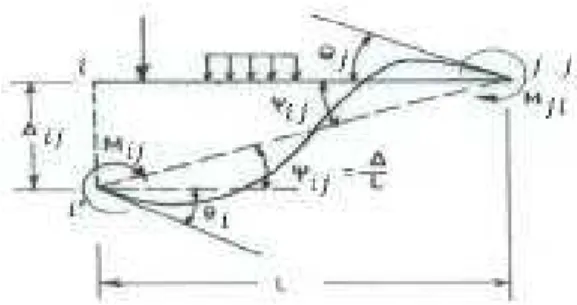
After finding nodal rotations, end moment and shear of members can be calculated using the slope deflection relations. These relations express end moment of a member based on rotations of nodes and elements, and also the external loads on the members. For element ij with constant bending rigidity, and length L (Figure 1), the relation is as follows (McCormac and Nelson, 1997; Norris et al., 1976).

Figure 1: Deformation curve of the elastic beam.

=2 _{! "2}Ѳ +Ѳ − 3& ' + ( (3)

=2 _{! "2}Ѳ +Ѳ − 3& ' + ( (4)

(5)

* = −6 _!_, "Ѳ +Ѳ − 2& ' + ( * (5)

* =6 _!_² "Ѳ +Ѳ − 2& ' + ( * (6)

Ѳ and Ѳ are the rotation of node i and j respectively, and φ shows the sway rotation of mem ber ij that is calculated through the below equation. FEM and FEV are the fixed end moment and shear. ) 7 (

& =

012

3

=

01 02

3

Δ_:Relative displacement of the member ends.

In Table 1, values of fixed end shear, moment and sign convention for different loading cases are shown(Mau, 2003):

FEM FEV Loads FEV FEM

−5!₈ 5₂ 52 5!₈

−7!₁₂, 7!₂ 7!₂ 7!₁₂,

Table 1: Values of fixed end shear and moment (Mau, 2003).

Also, Equations (3) to ( 6) could be written in matrix formulation (Megson, 2005):

9 : ;

*

* <=

> = ? @ @ @ @

ABCD3

,CD 3 ECD 3 ,CD 3 BCD 3 ECD 3 ECD 3F ECD 3F G,CD 3F ECD

3F ECD₃F G,CD₃F H

I I I I J

KLL

& M +

9 :

;(₍

( *

( * <=

>

(8)

By replacing the values of nodal displacements in the above matrix formulation, end shear force and moment of members are calculated. This matrix formation can be used in programming of the SDM matrix procedure.

(6)

* = − NOK _{+ O}K _{− PO + O Q& R + ( * (9)}

* = NOK + OK − PO + O Q & R + ( * (10)

where T and T are defined as follows:

O =V12W X21 V21

3 =

V12W X12 V12

3 =

V12 (GW X12 )

3 (11)

O =V21W X12 V12

3 =

V21W X21 V21

3 =

V21 (GW X21 )

3 (12)

In the above equations, C and C are moment carry over factors. Also, S and S are bending stiff ness values of the two ends of the non prismatic member and could be calculated by integration methods or using related handbooks(Association, 1958).

3 % + 1&'1' +( 11&' 4 0'1+ ( %& )% ' +% '( 5 ( 6

37$

SDM is an iterative method which is based on a series of computational cycles that are repeated until the results converge to a final value in each stage. By this repetition, simultaneous solving of algebraic equations is not necessary. This is a unique structural analysis method, in which the solu tion is obtained through an iterative process, without solving any equations to find problem param eters. SDM uses a Jacobi iterative scheme to find displacements in the system of equations pro duced by the slope deflection method.

37* ( 8

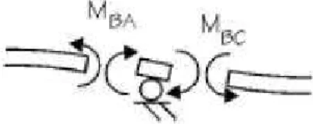
From static equilibrium, if external moment (M` ) is applied at the node B, the rotation at this node will take place until moment equilibrium is achieved, ∑ M_a_{= M}` (Figure 2).

Figure 2: Free body diagram for moment at node B (Lopes et al., 2011).

ab+ ac= Mde (13)

(7)

Mab= f2EI_{L j}

abk2Ѳa+ Ѳb− 3φabl + FEMab= f

4EI

L jab(Ѳa) − f

6EI

L jabφab+ FEMab (14)

Mac= f2EI_{L j}

ack2Ѳa+ Ѳc− 3φacl + FEMac= f

4EI

L jac(Ѳa) − f

6EI

L jacφac+ FEMac (15)

L is the length of the member, EI is the cross section rigidity, and

Ѳ

Bis the rotation at B

(Kassimali, 1995; Laursen, 1988).

Placing Equations (14) and (15) into equation (13) and solving for

Ѳ

B, we have:

Ѳa= Ma

` _{− FEM}

ab−FEMac

n4 EI_{L o}

ab+ n4 EIL oac

+ n6 EIL oab

n4 EI_{L o}

ab+ n4 EIL oac

φab+

n6 EI_{L o}_ac

n4 EI_{L o}

ab+ n4 EIL oac

φac (16)

In general, initial rotation of rigid node "i" has a direct relationship with the external load and the lateral rotation angle of members connected to the node. This dependency is shown in equation (17):

L(p)= de− ∑ (

qr qG

4 ( ∑qr_qGs ) + t 1.5 v

qr

qG

&(p) (17)

In the mentioned equation, N is the number of elements connected to node i, _R = y

∑z{_z y is the

relative bending stiffness of members connected to node i and K = (}~_•) is bending stiffness of each of these members.

In SDM, to calculate the slope of node i, the recursive series is defined as in equation (18):

θ(•)= θ(• G)+ Δθ(• G)= θ(p)+ t Δθ(ƒ)

ƒq• G

ƒqp

n ≥ 1 (18)

Where n is the number of analysis stage and θ(p) is the rotation value of node i under primary loads that are obtained through Equation (17). Δθ(ƒ)is the difference between the connection slope at node i, in two successive stages, due to incremental unbalanced moments. The value of Δθ(ƒ) will decrease during the analysis procedure and finally tends toward zero. In this condition, the connec tion rotation converges to its actual value, and the system will be balanced.

As discussed before, in the SDM method, incremental unbalanced moments at members’ ends decrease to achieve nodes’ equilibrium. In each step, for moment equilibrium condition at each node, it is necessary that: ∆M(•)= M` − ∑ Mq†_qG (•)→0.

Repeating the slope distribution approach, equilibrium is established in connection when n_→∞.

(8)

lead to change in rotation of this node in each cycle of the iterative procedure (_∆θ(•)). For nth Cy cle, ∆θ(•)is calculated through Equation (19).

∆‰_Š(‹)= ∆ŒŠ(‹)

• ∑•q••q‘ŽŠ•

=ŒŠ’“− ∑ ŒŠ•

(‹) •q• •q‘

• ∑•q••q‘ŽŠ•

(19)

Where, M` is external moment and ∑ Mq†_qG (•) is the sum of incrementally unbalanced moments at node i and ∑ Kq†_qG is the sum of the flexural stiffness of members connected to the ith node. n is the number of the analysis cycle and N is the number of members connected to node i. Equation (14) is obtained through a simple static equilibrium on node i. The equation is the same as the Ja cobi iterative procedure for solving the system of linear equations which has been described in pre vious parts. Using equation (19), the incremental unbalanced rotations caused by unbalanced mo ments, and consequently, the nodal rotations are calculated.

Inserting equations (3), (4) and (18) in equation (19), the fundamental equations of the SDM are consequently achieved:

ΔѲ(p)= t −1₂

q†

qG

R Ѳ(p) (20)

ΔѲ(•)= t −1₂

q†

qG

R ΔѲ(• G)+ t 1.5 R ”Δφ(• G)= φ(•)– φ(• G)– (21)

q†

qG

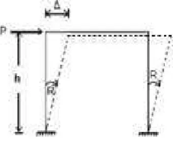
To compute the values of lateral rotation of the member ij,( φ(•)), a shear equilibrium equation should be used in each storey of the structure ( Figure 3).

Through writing static equilibrium in each storey of the structure (i.e. Sth storey), the auxiliary equation is obtained to analyze structure without forming any equation system:

*V = t *

q—

qG

(22)

In which, V_™is the shear of the Sth storey resulted from lateral loads such as earthquake or wind and V is the shear of the jth column of that storey and obtained through relations (5) and (6). The

φš(•)is calculated as follows:

&›(œ)= &›(p)+ t 0.5 • ”Ѳ(œ)+ Ѳ(œ)–

—

G

(9)

Latin American Journal of Solids and Structures 12 (2015) 2581 2617 Figure 3: The horizontal Shear of the frame in the Sth Storey (Rezaee Pajand and Aftabi Suny, 2010).

m is the number of columns in the Sth storey and i and j are the two ends of column ij; φ_š(p)is the initial rotation of member and D is the relative shear stiffness of the storey columns which is de fined through equations (24) and (25):

&›(p)=*V− ∑ ( *

— G

12 ∑ Ÿ—

G (24)

• = (_{∑ Ÿ}—Ÿ

G )V Ÿ = !¡¢ (25)

FEV is the fixed end shear of columns in the Sth storey; μ is shear stiffness of column ij, and D is the shear stiffness ratio of columns in the storey of interest.

The SDM method can be extended for the condition where the beams jointed to a node have a lateral displacement, and also when the φ values of structure members in a storey are not the same. As the lateral displacements of structural members (∆) in each storey are related by geometric rela tionships, the equations can be expressed based on the lateral rotation of a storey member (φ_™) that is considered as the base and independent one. So, the above equations will be corrected as follows:

L(p)= k de− ∑ (

qr qG

4 ∑ qr_qGs l + t 1.5 v

qr

qG

(&_&

V)&›

(p)₍₂₆₎

¤Ѳ(œ)= t −1₂

qr

qG

v ¤Ѳ(œ G)+ t 1.5 v &_&

V¢ ”¤&›

(œ G) _{= &}

›(œ)– &›(œ G)– (27)

qr

qG

&›(p)= *V− ∑ ( *

— G

12 ∑ (&_&

V)Ÿ — G

(10)

• = ( Ÿ

∑ (&&V)Ÿ

— G

)V (29)

In the above equations, N is the number of elements connected to node i, m is the number of col umns in the storey “S” and n is the step number of the recursive process.

As the lateral independent rotation of each storey of structure (φ_š(•)) is related to nodal rota tions (Ѳ(•)), we can place equation (23) into equation (27) and simplify the analysis stages:

ΔѲ(G)= t ω

q†

qG

ΔѲ(p)+ t ω¦ §t δ ”Ѳ© (G)+ Ѳ(G)–

G ª

q†

qG

(30)

For 2 ≤ n we have:

ΔѲ(•) = t ω

q†

qG

ΔѲ(• G)+ t ω¦ §t δ (ΔѲ© (• G)+ ΔѲ(• G))

G ª (31)

q†

qG

Where, ω = −G_,R and ω¦ = ”¬_¬

-– ω and R is the relative bending stiffness of members connect

ed to node i which was introduced before. Also, the value of the carry over factor (δ ) is defined as:

δ = −1.5 D .

The current equation performs as a recurrence relation. The rotation value of each node will be updated in each stage and finally converges to its accurate values. Closing the values of nodal rota tions in two consecutive steps by desired accuracy is considered as the end of the SDM process. If a structure has non prismatic members, then the above equations will be changed as follows:

L(p)= ( de− ∑ (

qr qG

∑qr_qG® ) + t 7¦

qr

qG

&V(p) (32)

¤L(p)= t 7

qr

qG

L(p) (33)

&›(œ)= &›(p)+ t •¯ Ѳ¯(œ)

—

G

(34)

Δθ(G)= t ω

q†

qG

Δθ(p)+ t ω¦ °t D± Ѳ±(G)

©

G

²

q†

qG

(11)

For n≥ 2 we have:

Δθ(•)= t ω

q†

qG

Δθ(• G)+ t ω¦

q†

qG

°tD±ΔѲ±(• G) ©

G

² (36)

ϕš(p)=V™ − ∑ FEV

© G

∑ ”φ_φ

š– T± ©

G

(37)

As the bending stiffness coefficients and carry over factor are different at two ends of storey col umns in non prismatic structures, the shear stiffness ratio (D_±) in node “r” of the column element should be calculated separately as follows:

•¯= O¯

∑ ”&&›– O¯

— G

(38)

T±is the shear stiffness of node “r” of the non prismatic column which is obtained through equations

(11) and (13), and ∑ T©_G _±is the total shear stiffness of all nodes of columns (nodes of the two ends of the columns) in the storey of interest (i.e. storey “s”) of the structure. Also, θ_± is the rotation of node “r” of the non prismatic column.

v = ®

∑ qr_qG® (39)

7 = − ´ v (40)

7¦ = P1 + ´ Q(&_&

›)v (41)

When the non prismatic structure has no lateral displacement in the storey “S”(φ_š= 0), by simplifi cation, the below relations are conducted:

Δθ(p)= t ω

q†

qG

θ(p) (42)

Δθ(•)= t ω

q†

qG

Δθ(• G) (43)

For a special situation, prismatic structure without any lateral displacement in the storey “S”

(12)

37, !

Sign convention in the proposed SDM method is similar to other manual analysis methods in which clockwise direction for θ,φ, FEM and M is considered as positive. According to this convention, the forces and linear displacements are taken as positive when the element rotates clockwise. It is in accordance with the positive directions used by some other researchers(e.g.(Timoshenko and Goodier, 1987). Also, the positive direction for shear force is the direction in which the force rotates the element clockwise (Figure 4).

Figure 4: Positive sign convention for force and displacement.

9 %& : -'& )0 % ' '- (

Manual approach of SDM should be repeated in a consecutive process until the final values of struc ture node displacements are obtained; this process is time consuming and boring in structures with high degrees of indeterminacy. In fact, in matrix formulation of SDM, the initial information such as(φ(p), θ(p), δ and ω) will be calculated manually by the user and a computer will be used to per form the analysis process. Therefore, introducing an accurate solution without any repetition proce dure and forming and solving only one matrix equation to give the unknowns, is the main purpose of the SDM matrix procedure.

If the equations (23), (25) and (26) are defined by matrix formulation, then we will have:

"∆θ(p)_{' = µω¶}^ _"θ(p)_{' (44)}

"ΔѲ(G)_{' = µω¶"∆θ}(p)_{' + µω¦¶µδ¶"θ}(G)_{' (45)}

If we have:

µτ¶ = µω¦¶µδ¶ (46)

And by inserting equation (46) in (47) we have:

"ΔѲ(G)_{' = µω¶}^F

"θ(p)_{' + µτ¶"θ}(G)_{' (47)}

(13)

factors of the members, and p is the number of rigid nodes and structure supports, and [Ι] is a unique matrix with an equal rank with [ω]. The matrices of µω¦¶ and µδ¶ have the same rank with

µω¶ and their entries are calculated just in two end nodes of the columns of each structure storey. They are replaced in corresponding matrixes to estimate the lateral displacement of structure (φ). In non prismatic structures, due to the difference between bending stiffness coefficients and carry over factors in two ends of storey columns, we have δ ≠ δ and they should be calculated separate ly for each column node. In a multi storey structure, µω¦¶and µδ¶ matrices should be formed separate ly for each storey of the structure and the matrix µτ¶ for all of the structure is calculated through the superposition principle by using the partial matrix of µτ¶ in each storey of the structure. There fore:

µτ¶ = ∑±q†-µτ¶_±

±qG (48)

In which, Ns is the number of stories in the structure.

Each row in matrix µω¦¶ is corresponded to the rigid node of structure storey, and the value of

µω¦¶ in node ί is equal to a total of (1 + C )R (»_»

-) for the members connected to node ί on the

storey “S”; which is placed in each entry of the ith row of matrix µω¦¶. Therefore:

µω¦¶™_{= tP1 + C} _Qφ

φš¢

q†

qG

R (49)

Indeed, the values of relative shear stiffness (_D_±), calculated through equation (38) are placed in matrix D, and matrix µδ¶ is obtained through equation (50):

)

50

(

¼δ ½ = ¼D ½ ⇒ µδ¶ = µD¶¿± •šÀÁš`

It should be noted that during the process of placing the entries in the global matrix of the struc ture, the zero value is considered for entries corresponding to nodes which do not exist in the given storey. If the structure includes prismatic members, equations (49) and (50) are changed as follows:

µω¦¶™_{= t}φ

φš¢

q†

qG

ω (51)

¼δ ½ = ¼−1.5 D ½ (52)

By calculating the above parameters, the rotations in structural nodes can be calculated. To this end, equation (27) can be changed to a matrix format. Equations (53) and (54) show the 2nd step of calculating ΔѲ:

(14)

"ΔѲ(,)_{' = (µ}ω¶ + nτ_o)^ _NΔѲ(G)_{R (54)}

In this way, through expanding relationship (27), other values of "ΔѲ(•)' can be obtained for n≥ 2:

"ΔѲ(•)_{' = (µω¶ + ¼τ½)}^ Â _"ΔѲ_(G)_{' (55)}

Then, through placing equations (44), (45) and (55) in (18), the values of "θ(•)' will be calculated in the last cycle. Therefore, it can be concluded that:

kθl = ¼(µI¶ + µω¶) + µ µI¶ − (µω¶ + µτ¶) ¶ G_{× (µω¶}^F

+ µτ¶(µI¶ + µω¶))½"θ(p)_{' (56)}

If we define: µZ¶ = InversekµI¶ − µV¶l , µV¶ = µω¶ + µτ¶ and µU¶ = µI¶ + µω¶, then we will have:

kθl = nµU¶ + µZ¶Pµω¶^F

+ µτ¶µU¶Qo "θ(p)_{' (57)}

Final values of nodal rotations can be calculated through equation (56) by forming and solving only one matrix equation. End moments and shears of members can be evaluated through placing the nodal rotations in slope deflection equations. The above equation can be used in computer pro gramming of SDM. It should be noted that the slope distribution factors in matrix formulations of SDM are calculated for all members connected to the structure nodes, whereas the supports will also be considered as nodes. At first, to compute the bending stiffness, carry over factors of mem bers and fixed end moments for non prismatic members, the “hand book of frame constants”((Association, 1958)) could be used. Then, the matrix of slope distribution factor, [ω], will be formed for a structure. This matrix is a square one with a rank of (p×p), where p is the number of structure nodes. The entry_ω in matrix [ω] is equal to the slope distribution factor of member ij, which connects the nodes i and j. For those nodes which are not connected to each other by any member, ω = 0; for original diameter entries, ω = 0 and for fixed and two roller supports in which R = 0, ω is also considered as zero. For hinge and roller supports, ω = − C , because the value of R is equal to unity (see equation (40)). The value of initial rotation for a rigid node of structure under external loading is obtained by equations (26) and (32). For fixed and two roller supports, θ(p)= 0 and for hinged support and roller support, it is computed through equation (26). It is worth noting that the initial rotation value in matrix formulation of SDM is computed for a hinged support; So, the bending stiffness, carry over factor and the fixed end moments obtained through “handbooks of frame constants” ((Association, 1958)) will be used in the equations without any changes. If the structure has no lateral displacement (φ = 0), equation (56) will be simplified as follows:

kθl = ¼µI ¶ − µ ω¶½ G kθ(p)_{l (58)}

; ) +& 0 +: 10+

(15)

A and D are fixed. Other specifications are shown in Figure 5. The cross section of beam is U shape (UPN 80).EI is assumed to be constant through the length of the beam.

Figure 5: Continuous beam with asymmetric loading (Lopes et al., 2011).

Fixed end moment of members and initial rotation of the structure nodes and slope distribution factors are calculated in Table 2:

D C

B A

Node

DC CD

CB BC

BA AB

Member

0 0

133.225 133.225

63.875 63.875

FEM

0 81.0452/EI

63.282/EI 0

L(p)

0 0.3333

0.1666 0.25

0.25 0

ω

Table 2: Fixed end moment, initial rotations and slope distribution factors for the example 6.1.

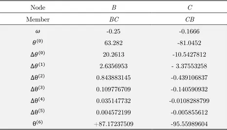
Table 3 shows the steps of Jacobi based SDM for analysis of the continuous beam of example 6.1:

C B

Node

CB BC

Member

0.1666 0.25

7

81.0452 63.282

L(p)

10.5427812 20.2613

ΔL(p)

3.37553258 2.6356953

ΔL(G)

0.439106837 0.843883145

Δθ(,)

0.140590932 0.109776709

Δθ(Ç)

0.0108288799 0.035147732

Δθ(B)

0.005855612 0.004572199

Δθ(È)

95.55989604 +87.17237509

θ(E)

(16)

Below, the parametric calculation of some steps of the SDM is shown:

¤LÉp= 7ÉX LXp , ¤LXp= 7XÉ LÉp, ¤LÉG= 7ÉX ¤LXp , ¤LXG= 7XÉ ¤LÉ ,p ¤LÉ,= 7ÉX ¤LXG , ¤LX,= 7XÉ ¤LÉG

Using slope deflection relations, the values of end moments and shears for the beam are calculated as below:

MAB= 39.9921, MBA=111.6406, MBC= 111.6401, MCB=104.7462, MCD= 104.7231, MDC= 52.3615, VAB=25.1851, VBA=44.8148, VBC=110.4443, VCB=108.5556,

VCD=43.0369, VDC= 43.0369.

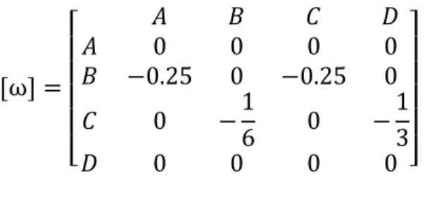
To apply the matrix formulation on the above example, [ω] and kθpl are formed for the beam of Figure 5, by using the parameter values in Table 2:

µω¶ =

?

@

A

_Ê

Ê

₀

Ë

₀

´

₀

• ₀

Ë −0.25

0 −0.25

0 ´

0 −

1 ₆

0 −

1 ₃

•

0

0 0 H

I

J

By applying equation (58) and using the calculated [_ω] and_kθp_l, nodal rotation matrix is obtained as follow:

k

L(0)

_{l =}

9 Ì

:

Ì

;

Ê = 0

Ë =

63.282 ´ =

−81.0452

• = 0

<

Ì

=

Ì

>

⇒ kLl =

9 Ì

:

Ì

;

Ê = 0

Ë =

87.1756

´ =

−95.5744

• = 0

<

Ì

=

Ì

>

As could be seen, the results of the manual and matrix formulation are in good agreement. The above beam is also analyzed by Sap2000 software. The results are shown in Figures. 6 and 7.

(17)

Latin American Journal of Solids and Structures 12 (2015) 2581 2617 Figure 7: Bending moment diagram (KN.m) for the beam of the example 6.1.

As can be seen, the difference between the results of the SDM with those of these diagrams is negli gible and is less than 1% .It seems this small difference is because of considering shear deformation in software calculations.

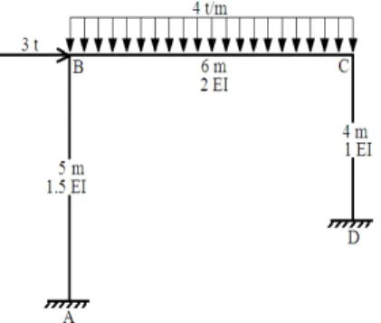
6.2 In this example, bending frame with lateral displacement and different columns heights, will analyze by classic and matrix procedure of SDM and results will be compared with those of Sap2000 software. Characteristics, loading and support conditions are shown in Figure 8 and the flexural rigidity of frame members is constant.

Figure 8: The Frame with different column heights (example 6.2).

If it is supposed that φ_ba is considered as the independent φ of the storey, and we have: φ_š=_φ_ba, then regarding geometric relationships between the members of the frame, it can be obtained that:

+1.25ϕš

=

φcÍ

and

0

=

φac

At first, primarily needed parameters are calculated. These values are presented in Table 4.

D C

B A

Node

DC CD

CB BC

BA AB

Member

0 0

12 12

0 0

FEM

0 −3.6884/EI

6.023/EI + 0

L(p)

0 0.4286

0.5714 0.5263

0.4737 0

R

0 0.21428

0.2857 0.2631

0.2368 0

7

0 0.26785

0.2368 0

7¦

0.6787 0.6787

− − − − − − − −

0.6516 0.6516

Î

(18)

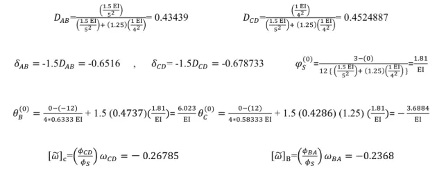
•ÏÉ= ”

.Ð ÑÒ ÐF –

” .Ð ÑÒ_ÐF –W (G.,È)”_ÓF ÑÒ–= 0.43439 •XÔ=

”_ÓF ÑÒ–

”.Ð ÑÒ_ÐF –W (G.,È)”_ÓF ÑÒ–= 0.4524887

ÎÏÉ= 1.5•_ÏÉ= 0.6516 , Î_XÔ= 1.5•_XÔ= 0.678733 &_V(p)= Ç (p)

G, k ” .Ð ÑÒ_ÐF –W (G.,È)”_ÓF ÑÒ– l= G.ÕG

}~

LÉ(p)=_{B∗p.EÇÇÇ }~}p ( G,) + 1.5 (0.4737)(G.ÕG_}~)= E.p,Ç_}~ LX(p)=_{B∗p.ÈÕÇÇÇ }~}p (G,) + 1.5 (0.4286) (1.25) (G.ÕG_}~)= −Ç.EÕÕB_}~

µ7¦¶×=”Ø_ØÙÚ

Û– 7XÔ=

−

0.26785 µ7¦¶a=”

ØÜÝ

ØÛ– 7ÉÏ= −0.2368

Now, slope distribution relationships between rigid nodes are simply produced through computing needed parameters. The parametric form of the slope distribution procedure for calculating nodal rotations of Figure 8 is shown in Table 5 (for the first three steps). Similarly, by repeating this pro cedure, other step values of nodal rotations’ changes are calculated. The results of all stages are shown in Figure 9.

C B

Node

7XÉLÉ(p)

7ÉXLX(p)

∆L(p)

7XÉ∆LÉ(p)+ 7¦cnÎÏÉLÉ(G)+ ÎXÔLX(G)o

7ÉX∆LX(p)+ 7¦anÎÏÉLÉ(G)+ ÎXÔLX(G)o

∆L(G)

7XÉ∆LÉ(G)+ 7¦cnÎÏÉ∆LÉ(G)+ ÎXÔ∆LX(G)o

7ÉX∆LX(G)+ 7¦anÎÏÉ∆LÉ(G)+ ÎXÔ∆LX(G)o

∆L(,)

Table 5: Parametric form of SDM procedure for calculating nodal rotation of example 6.2.

(19)

Now, for the matrix procedure of SDM, by calculating the required parameters, the corresponding matrices can be formed. Then, through SDM matrix procedure, frame node rotations will be de fined:

µω¶ =

? @ @ @

A_Ê Ê₀ Ë₀ ´₀ •₀

Ë −0.236842 0 −0.263158 0

´ 0 −0.285714 0 −0.214286

• 0 0 0 0 HI

I I J

µ7¦¶ = Þ

0 0 0 0

−0.236842 −0.236842 −0.236842 −0.236842 −0.267857 −0.267857 −0.267857 −0.267857

0 0 0 0

ß

µδ¶ = Þ

0 −0.6516 0 0

−0.6516 0 0 0

0 0 0 −0.678733

0 0 −0.678733 0

ß

"L(p)_{' =}

9 Ì : Ì

; Ê = 0

Ë =6.023

´ = −3.6884

• = 0 <Ì

= Ì >

⇒ kLl =

9 Ì : Ì

; Ê = 0

Ë =7.7963

´ = −5.56734

• = 0 <Ì

= Ì >

As can be observed, the calculated nodes rotation values through manual procedure of SDM after the sixth stages are equal to the results from their matrix procedure, till two decimals value; this shows the proper accuracy and convergence of the proposed method. Now, the lateral rotation of members, end moment and end shear values of members can be computed using equation (23) and slope deflection relations:

&

V

+

,.,BB_}~

= 0.64, = 5.32, = 5.32, =9.77, = 9.77, = 7

=1.2→, =1.2←, = 11.257↑, =12.743↑, = 4.2→, =4.2←

(20)

Figure 10: The shear diagram (in Ton) and moment diagram (in Ton m) of the frame of example 6.2

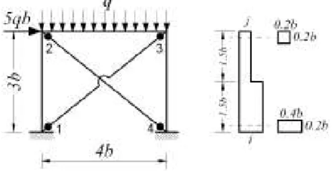
6.3 In this example, one single bay moment resisting frame with a single storey is considered which has non prismatic columns and a set of cross bracing (x bracing)(Rezaee Pajand and Aftabi Suny, 2010). As is clear in Figure 11, the frame has a bay of 4b and a height of 3b. Columns of frame are non prismatic with two different end sections as shown in the figure and its beam is prismatic with a section like the column in connecting joint. The beams and columns of the frame are made from materials with an elastic modulus of 10E. On the other hand, braces have an elastic modulus of E and a section area of 0.01b2.

Figure 11: The one bay moment resisting frame with non prismatic columns and x bracing system(Rezaee Pajand and Aftabi Suny, 2010)

In such a problem, the stiffness of braces in the storey should be included in calculations. What analyzing relations reveals is, while designing of the two given bracing members is performed based on allowable compression force, both members will participate in the lateral resisting system; so, the total lateral stiffness of the braces is equal to total lateral stiffness of the two members (Rezaee Pajand and Aftabi Suny, 2010; Zalka, 2002):

Figure 12: A X bracing frame(Rezaee Pajand and Aftabi Suny, 2010).

M.

Diagram

Dig

(21)

sâ = 2sÉ¯ãäd= 2 ( _{! ) åæç}Ê ,L (59)

Where, E is elasticity modulus, A is cross section area, L, is the length of bracing member and Ө is the angle between the bracing member axis and horizontal direction. Regarding that the above sys tem is a dual bending–bracing frame system, it is needed to consider the stiffness of these two sys tems during the computations processes, simultaneously. According to Figure 3, the storey shear (V_š) is equal to the sum of the column’s shear forces and the horizontal components of the bracing members forces in the desired storey:

*â+ t *

—

G

= *› (60)

In which, m is the number of column members in the storey and V_è is obtained by the below equa tion:

*_â = s_â∆_› (61)

In this equation, the sum of lateral stiffness of the bracing system in the Sth storey is defined by K_è. According to Figure 4 and based on the main assumption of the SDM method, i.e. neglecting axial deformation of frame members, relative displacements of all Sth storey columns are the same and equal to ∆_š.

All bending frame equations are used in dual frames, but member shear stiffness will be changed. Therefore equations (28) and (29) are modified as follows:

•¯= O¯

( sâéš) + ∑ (—G &_&_›) O¯

(62) &›(p)= *V − ∑ ( *

— G

( sâéš) + ∑ (—G &_&_›) O¯

(63)

If the structural members are prismatic, the above equations will be simplified as below:

• = Ÿ

( sâéš

12 ) + ∑ (&&›)Ÿ

— G

(64) &›(p)= *V − ∑ ( *

— G

( sâéš) + 12 ∑ (—G &_&_›)Ÿ

(65)

Now, to solve the above problem, stiffness and carry over coefficients of non prismatic columns are computed at first, using the tables of “handbook of frame constants” (Association, 1958), as fol lows:

®G,= 20.61 ê(10 )((0.2 ë)

B

12 )

(22)

®,G= 5.42 ê(10 )((0.2 ë)

B

12 )

3ë ì = 0.00241 ëÇ= ®ÇB

The frame beam is prismatic and has stiffness coefficient and carry over factors as below:

®,Ç= 4 ê(10 )((0.2 ë)

B

12 )

4ë ì = 0.0013333 ëÇ= ®Ç,

sâ = 2 (0.01 ë

,₎

5ë (45),= 0.00256 Eb sâ é›= 0.00768 ë,

Now, by defining the required data, the rotation coefficients are calculated:

v,G=_{∑ ®}®,G

,=

0.00241 ëÇ

0.00241 ëÇ_{+ 0.0013333 ë}Ç= 0.64381122 = vÇB

7,G= −´,G v,G= − 0.77257 = 7ÇB

v,Ç=_{∑ ®}®,Ç

,=

0.0013333 ëÇ

0.00241 ëÇ_{+ 0.0013333 ë}Ç= 0.3562 = vÇ, 7,Ç= −´,Ç v,Ç= − 0.1781 = 7Ç,

OG=®G,+ ´_! ,G®,G

G, = 0.00402 ë

,_{= O}

B O,=®,G+ ´_! G,®G,

G, = 0.00177 ë

,_{= O} Ç

( sâéš) + t k (í_í

›) ( O¯ ) l =

—

G

0.01926 ë,

•G= 0.208723 = •B •,= 0.0919 = •Ç

µ7¦¶,= (1 + ´,G)v,G &_&,G

V¢ = 1.4164 = µ7¦¶Ç

&_V(p)=_{0.01926 ë}5îë − 0 _,= 259.6054 î_ë

L_,(p)=0 – (− ” 43– îë_{0.0037433 ë},_Ç) + (1 + 1.2)(0.64381122)(259.6054 î_{ë) = 723.89387} î_ë

LÇ(p)= 0 – (” 43– îë

,₎

(23)

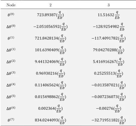
Latin American Journal of Solids and Structures 12 (2015) 2581 2617 3

2 Node

7Ç,L,(p)

7,ÇLÇ(p)

∆L(p)

7Ç,∆L,(p)+ 7¦Çn•,GL,(G)+ •ÇBLÇ(G)o

7,Ç∆LÇ(p)+ 7¦,n•,GL,(G)+ •ÇBLÇ(G)o

∆L(G)

7Ç,∆L,(G)+ 7¦Çn•,G∆L,(G)+ •ÇB∆LÇ(G)o

7,Ç∆LÇ(G)+ 7¦,n•,G∆L,(G)+ •ÇB∆LÇ(G)o

∆L(,)

Table 6: Parametric form of SDM procedure for nodal rotation of example 6.3.

3 2

Node

11.51632 î_ë 723.89387(î_ë)

L(p)

−128.9254982 î_ë

−2.051056592(î_ë)

∆L(p)

−117.4091782(î_ë)

721.8428134(î_ë) L(G)

79.04270288(î_ë) 101.6390409(î_ë)

∆L(G)

5.416916267(î_ë) 9.441324069(î_ë)

∆L(,)

0.25255513(î_ë) 0.96930216(î_ë)

∆L(Ç)

−0.013587021(î_ë)

0.114065624(î_ë) ∆L(B)

−0.007236073(î_ë)

0.015498862(î_ë) ∆L(È)

−0.00276(î_ë) 0.002364(î_ë)

∆L(E)

−32.71951182(î_ë)

834.0244093(î_ë) L(ï)

Table 7: The results of SDM procedure for nodal rotation of example 6.3.

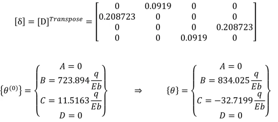
By calculating the required parameters, the corresponding matrices for the structure are formed:

µω¶ = Þ

0 0 0 0

−0.77257 0 −0.1781 0

0 −0.1781 0 −0.77257

0 0 0 0

ß

µ7¦¶ = Þ

0 0 0 0

1.4164 1.4164 1.4164 1.4164 1.4164 1.4164 1.4164 1.4164

0 0 0 0

(24)

µδ¶ = µD¶ð¯ãœ›ñò›d_{= Þ}

0 0.0919 0 0

0.208723 0 0 0

0 0 0 0.208723

0 0 0.0919 0

ß

"L(p)_{' =}

9 Ì : Ì

; Ê = 0

Ë = 723.894 î_ë

´ = 11.5163 î_ë

• = 0 <Ì

= Ì >

⇒ kLl =

9 Ì : Ì

; Ê = 0

Ë = 834.025 î_ë

´ = −32.7199 î_ë

• = 0 <Ì

= Ì >

Through comparing manual and matrix procedures of SDM, it can be shown that the value of frame nodal rotation after the sixth step using a manual procedure is equal to its matrix results till two decimal values which indicate the accuracy and good convergence speed of the proposed meth od.

After calculating the nodal displacements, members’ lateral rotations and bending moments are resulted by equation (34) and slope deflection equation, respectively:

&V= 333.24533 ”î_ë–

G,= −1.603 îë,, _,G= 0.2431 îë,, _,Ç= −0.2431îë,, _Ç,= 1.846 îë,, _ÇB= −1.846 îë,,

BÇ= −4.112 îë,

In the above example, if the bracing system is eccentric, the only difference is the value of the stiff ness of bracing members. Regarding studies (Rezaee Pajand and Aftabi Suny, 2010; Zalka, 2002), it is just enough that parameter “A” in equation (59) is replaced by "A_`" which is defined as follows:

Figure 13: An eccentric bracing frame(Rezaee Pajand and Aftabi Suny, 2010).

Êd = õ,ö1 + ÷

,

õ,_{+ ÷},ø

Ç ,

Ê (66)

(25)

These two factors can be seen in Figure 13. In a situation where shear walls are used in the struc ture, it is just enough to define wall lateral stiffness through the following equation to analyze the structure by the SDM method:

Kû=_γH3EI_Ç (67)

Where, E is elasticity modulus for concrete shear wall and I is the moment inertia of shear wall and are calculated by following equation:

E = 5000þF f× (68)

I =bL_{12 (69)}Çû

f×is compressive strength of concrete based on N/mm2 . b and Lû are the thickness and the length

of the wall, respectively. Coefficient γ in equation (67) shows the effect of shear deformation on the wall stiffness and obtained by the following equation:

γ = 1 + 0.75 L_{H ¢ (70)}û

where, H is the height of the wall.

< + ( = -& + / % ' .+&% 0 '0) 7

<7$

The SDM method can be used for frames at which the beams at storey level have lateral rotation or the columns are non vertical. Through writing horizontal equilibrium equations for shear force, the horizontal components of the axial forces of non vertical columns are participated in the equilibri um. Therefore, to ease the process, moment equilibrium equation around a virtual point resulted from the intersection of members or the continuation (point I in Figure 14), are used to remove the effect of column axial force in equations. If the concentrated load of P is applied on the connection “B” in the frame of Figure 14, the parameters of the SDM approach can be defined for the frame through writing moment equilibrium for point “I”.

(26)

As mentioned in (Kaveh, 2012), lateral displacements of members can be simply described based on frame independent displacement through geometric relationships. This dependency is defined for the frame of Figure 14 by following equations:

∆G

ç L =ç (90∆°, − L) =ç 90∆Ç ° (71)

∆G= ∆, L = ∆Çç L (72)

Lateral rotation of member “AB” is supposed as the basis (_φ_š=_φ_ba ) and the length of h and r is equal to r =_×Áš• and h=L_actan θ, therefore:

&V(p)=

5 ”ℎ– − ”( ÏÉ+ ( ÔX_{– − ( *}ÏÉ(é +ℎ) + ( *ÔX(v + )¢

12 §” _é,– n”ℎ– + ” é_{2 –o + ”}_v,– ”&_&ÔX_V– n1 + ” v_{2 –oª}

(73)

Also, the relative shear stiffness and lateral rotation of members are defined as follows:

•ÏÉ=

” _é,– n”ℎ– + ”2é_{3 –o}

” _é,– n”ℎ– + ” é_{2 –o + ”}_v,– ”&_&ÔX_V – n1 + ” v_{2 –o}

(74)

•XÔ=

” _v,– n1 + ”2v_{3 –o}

” _é,– n”ℎ– + ” é_{2 –o + ”}_v,– ”&_&ÔX_V – n1 + ” v_{2 –o}

(75)

&_V(œ)= &_V(p)+ 0.5 •ÏÉ”ѲÏ(œ)+ ѲÉ(œ)– + 0.5 •XÔ”ѲX(œ)+ ѲÔ(œ)– (76)

It can be seen that if θ →_,, then r&h→∞ ,

± →1 and G

± →0 and the equations will be simplified.

(27)

Latin American Journal of Solids and Structures 12 (2015) 2581 2617 Figure 15: Frame of example 7.2 and the structure characteristics(Kaveh, 2012).

If φ_š=_φ_ba, then from equation (72), we have the following relations:

In this example, the required parameters are calculated firstly and the structure is analyzed by the two manual and matrix forms of the proposed method.

D C

B A

Node

DC CD

CB BC

BA AB

Member

0 0

FEM

0 0

20.4082 0

L(p)

0 1

2 1

2 2

3 1

3 0

R

0 − 1₄

− 1₄ − 1₃

− 1₆ 0

7

0.81632 0.81632

0.4898 0.4898

D

1.22449 1.22449

0.7347 0.7347

Î

0 0

0.08333 0

7¦

Table 8: Fixed end moment of the members, slope distribution and carry over factors of the frame of Figure 15.

φ_V(p)= 100 ”2025– − (0) − (0)

12 k ”0.5_{15– n”}20_{25– + ”}_{2 ∗ 25–o + ”}15 _{25– (0.75) n1 + ”}1 _{2 ∗ 25–o l}25 = 81.6326

•ÏÉ= ”

.Ð

Ð–n”FFÐ–W”F∗ Ð∗FÐ–o

”.Ð_Ð–n”F_FÐ–W”_F∗FÐÐ–oW ”_FÐ–(p.ïÈ)nGW”_F∗FÐFÐ–o= 0.4898 •XÔ=

”_FÐ–nGW”F∗FÐ_∗FÐ–o

(28)

ÎXÔ= 1.5•XÔ=1.22449 ÎÏÉ = 1.5•ÏÉ = 0.7347

LX(p)={(1.5)( 0.75)”G_,–+(1.5)(0.75)”G_,–}(81.6326)= 0 , LÉ(p)={1.5”G_Ç–+(1.5)( 0.75)”,_Ç–}(81.6326)=

20.4082

7¦a=”Ø_ØÜÝ_Û– 7ÉÏ + ”Ø_ØÜÙ_Û– 7ÉX=0.08333 , 7¦ = öφ_φÙÜ

Ûø 7XÉ + ”

ØÙÚ

ØÛ– 7XÔ= 0

Now, through calculating required parameters, the slope distribution process will be repeated be tween rigid connections. Parametric form of slope distribution procedure for calculating nodal rota tion of the frame of Figure 15 is similar to Table 5. In Table 9, the calculation process of the rota tions for nodes B and C are presented:

C B

Node

0 −20.4082

L(p)

5.10505 0

∆L(p)

5.10505 −20.4082

L(G)

0 −0.971813

∆L(G)

0.243 0.0595

∆L(,)

−0.014875 −0.10944

∆L(Ç)

0.02736 0.013176

∆L(B)

−0.00323 −0.01272

∆L(È)

5.3542 −21.4295

L(E)

Table 9:Calculation process of the rotation values for nodes B and C of the frame of Figure 15.

For analysis of the frame by matrix formulation of the presented approach, the corresponding ma trices should be formed at first:

µω¶ = ? @ @ @

A 0 0 0 0

−1₆ 0 −1₃ 0

0 −0.25 0 −0.25

0 0 0 0 HI

I I J

µ7¦¶ = Þ

0 0 0 0

0.08333 0.08333 0.08333 0.08333

0 0 0 0

(29)

µδ¶ = Þ

0 −0.7347 0 0

−0.7347 0 0 0

0 0 0 −1.22449

0 0 −1.22449 0

ß

By forming the initial rotation matrix and using equation (56), the final rotation value of the nodes are calculated:

"L(p)_{' =}

Ê = 0 Ë = −20.4082

´ = 0 • = 0

⇒ kLl =

Ê = 0 Ë = −21.4286

´ = 5.35715 • = 0

By using equation (23) and applying slope deflection equations, the end moments and shears of the members are calculated.

MAB= 257.8923, MBA= 279.321, MBC= 279.695, MCB=333.267, MCD= 333.267, MDC= 344

VAB=35.8142←, VBA=35.8142→,VBC= 40.864↓, VCB=40.864↑, VCD= 27→, VDC=27←

The comparison of the results with those of (Kaveh, 2012), shows the accuracy of the proposed method.

> + ( = -& + / % .+&% 0 ( 10 + + % '- % + '(+

>7$

If a frame column does not continue to the foundation level, due to vertical displacements, the frame beams will have lateral rotation. This is a limitation of the Kani method which is not able to analyze a frame with vertical displacement, and structure columns should be continued to the foun dation level. But through the SDM method, these kinds of structures can be analyzed. An example of this structure is shown in Figure 16.

(30)

In this condition, through writing the shear equilibrium equation in vertical direction (Figure 17) and replacing the end shear of members, an auxiliary equation will be obtained. This equation con siders the vertical displacement, ₃, and consequently the lateral rotation of the beam (

ϕ

₃):

Figure 17: The free diagram of a part of the frame of Figure 16.

) 77 (

V_cÍ+ V_a}+ V _Í+ V _}= F_de

F` , is the resultant of external forces in vertical direction which are applied on the frame part that

is shown in Figure 17. Through simplifying, the below auxiliary equation will be obtained:

&Ç(œ)= &Ç(p)+ 0.5 •ÉC”ѲÉ(œ)+ѲC(œ)– +0.5 •XÔ”ѲX(œ)+ѲÔ(œ)– −0.5 • Ô”Ѳ(œ)+ѲÔ(œ)–

−0.5 • C”Ѳ(œ))+ѲC(œ)–

&_Ç(p)= F` − ∑ ( *

12 k ”&ÉC

&Ç– ŸÉC + ”&

XÔ

&Ç– ŸXÔ− ”&

C

&Ç– Ÿ C − ”&

Ô

&Ç– Ÿ Ôl

(79)

• = Ÿ

”&ÉC

&Ç– ŸÉC + ”&

XÔ

&Ç– ŸXÔ− ”&

C

&Ç– Ÿ C − ”&

Ô

&Ç– Ÿ Ô

, Ÿ = _!_¡¢ (80)

It should be noted that the geometrical relations between structural members are as follows:

φa}= +_L∆Ç

a}, φcÍ= +

∆Ç

LcÍ, φ }= −

∆Ç

L }, φ Í= −

∆Ç

L Í

In the following example, the classical and matrix computing stages of SDM in a frame with verti cal displacement are explained more:

8.2. In this example, a two storey bending frame containing horizontal and vertical displacement is evaluated through classical and matrix approach of SDM. This frame is influenced by uniform dead

(31)

load and horizontal force resulted from an earthquake. The frame geometrical characteristics and loading are represented in Figure 18. Finally, the obtained results will be compared with those of SAP2000 software. Bending rigidity values of all frame members are constant and equal.

Figure 18: The bending frame of Figure 17.

Considering the geometrical relation between structural members, we have:

&ÏÉ= & = +& G, &ÉX= &CÔ = & = +& , , &ÉC = &XÔ= +&Ç , &C = &Ô = − &Ç

The required coefficients and factors are calculated through simple relations of structural analysis (Tables 10 and 11).

H D

C A , F

Node HG HD DH DE DC CD CB AB , FG Member 0 2.25 2.25 0 2.25 2.25 0 0 FEM 1.7777/EI 2.25/EI 2.25/EI 1.7777/EI 2.25/EI 2.25/EI 1.7777/EI 4/EI φ(p) 1.74983/EI 0.727273 /EI 4.035694 /EI 0 θ(p) 0.4286 0.5714 0.3636 0.2727 0.3636 0.5714 0.4286 0 R 0.2143 0.2857 0.1818 0.1364 0.1818 0.2857 0.2143 0 7 0.3333 0.25 0.25 0.3333 0.25 0.25 0.3333 0.5 D 0.5 +0.375 +0.375 0.5 0.375 0.375 0.5 0.75 Î

(32)

G E B Node GF GH GE EG ED EB BC BE BA Member 0 0 0.75 0.75 0 0.75 0 0.75 s0 FEM 4/EI 1.7777/EI 2.25/EI 2.25/EI 1.7777/EI 2.25/EI 1.7777/EI 2.25/EI 4/EI φ(p) 1.025 /EI 0.727273 /EI 4.175/EI θ(p) 0.3 0.3 0.4 0.3636 0.2727 0.3636 0.3 0.4 0.3 R 0.15 0.15 0.2 0.1818 0.1364 0.1818 0.15 0.2 0.15 7 0.5 0.3333 0.25 0.25 0.3333 0.25 0.3333 0.25 0.5 D 0.75 0.5 +0.375 +0.375 0.5 0.375 0.5 0.375 0.75 Î

Table 10 (cont.): Fixed end moment of members, slop distribution and carry over factors for example 8.2.

H G E D C B

A , F Node

0.15 0.15

0 Due to

ϕ

₁

7¦ values for

each node Due to

ϕ

₂ 0.15 0.2143 0.1364 0.1364 0.15 0.2143

+0.2857 +0.2 `0 0 0.2857 0.2

Due to

ϕ

₃

Table 11: 7¦ values for nodes in the structure of Figure 18.

Through computing required parameters, the classical iterative procedure of SDM is repeated through structure rigid nodes till changes in nodal rotations values become negligible in two succes sive steps. The results are shown on Figure 19.

As EI is constant and equal for all frame members, it is not shown in Figure 19. The final values of rotations should be divided by this parameter. Through the sum of partial rotations calculated in each node, the values of final node rotations and also, the member lateral rotations are obtained:

LÏ(ï)= 0_{, L}É(ï)=6.16457_, LX(ï)=4.86486_{, L}Ô(ï)=1.12757

L_C(ï)=−0.171009 , L(ï)= 0_, L(ï)=2.45871_, L(ï)=−2.4981

(33)

Latin American Journal of Solids and Structures 12 (2015) 2581 2617 Figure 19: Classical procedure of SDM for analysis of the frame of example 2.8.

For analysis of the frame by matrix procedure, the corresponding matrices are formed firstly based on Tables 10 and 11.

µω¶ =

? @ @ @ @ @ @

A_−0.150 0₀ _−0.150 0₀ _−0.20 0₀ ₀0 0₀

0 −0.2143 0 −0.2857 0 0 0 0

0 0 −0.1818 0 −0.1364 0 0 −0.1818

0 −0.1818 0 −0.1364 0 0 −0.1818 0

0 0 0 0 0 0 0 0

0 0 0 0 −0.2 −0.15 0 −0.15

0 0 0 −0.2857 0 0 −0.2143 0 HI

I I I I I J

µω¦¶G=

? @ @ @ @ @ @

A_{−0.15 −0.15 0 0 −0.15 −0.15 −0.15 0}0 0 0 0 0 0 0 0

0 0 0 0 0 0 0 0

−0.15 −0.15 0 0 −0.15 −0.15 −0.15 0

0 0 0 0 0 0 0 0HI

(34)

µδ¶G=

? @ @ @ @ @ @

A 0_−0.75 −0.75 0 0 0₀ _{0 0 0} 0₀ 0₀ 0₀

0 0 0 0 0 0 0 0

0 0 0 0 0 0 −0.75 0

0 0 0 0 0 −0.75 0 0

0 0 0 0 0 0 0 0HI

I I I I I J

µω¦¶,=

? @ @ @ @ @ @

A0₀ _−0.150 _−0.150 _−0.150 _−0.150 0₀ _−0.150 _−0.150

0 −0.2143 −0.2143 −0.2143 −0.2143 0 −0.2143 −0.2143 0 −0.1364 −0.1364 −0.1364 −0.1364 0 −0.1364 −0.1364 0 −0.1364 −0.1364 −0.1364 −0.1364 0 −0.1364 −0.1364

0 0 0 0 0 0 0 0

0 −0.15 −0.15 −0.15 −0.15 0 −0.15 −0.15

0 −0.2143 −0.2143 −0.2143 −0.2143 0 −0.2143 −0.2143HI

I I I I I J

µδ¶,=

? @ @ @ @ @ @

A0₀ 0₀ _−0.50 0₀ 0₀ 0₀ ₀0 0₀

0 −0.5 0 0 0 0 0 0

0 0 0 0 −0.5 0 0 0

0 0 0 −0.5 0 0 0 0

0 0 0 0 0 0 0 0

0 0 0 0 0 0 0 −0.5

0 0 0 0 0 0 −0.5 0 HI

I I I I I J

µω¦¶Ç=

? @ @ @ @ @ @

A0₀ _−0.20 _−0.20 _−0.20 _−0.20 0₀ _−0.20 _−0.20

0 −0.2857 −0.2857 −0.2857 −0.2857 0 −0.2857 −0.2857

0 0 0 0 0 0 0 0

0 0.2 0.2 0.2 0.2 0 0.2 0.2

0 0.2857 0.2857 0.2857 0.2857 0 0.2857 0.2857 HI

I I I I I J

µδ¶Ç=

? @ @ @ @ @ @

A0₀ 0₀ 0₀ 0₀ _−0.3750 0₀ ₀0 0₀

0 0 0 −0.375 0 0 0 0

0 0 −0.375 0 0 0 0 0.375

0 −0.375 0 0 0 0 0.375 0

0 0 0 0 0 0.375 0 0

0 0 0 0 0.375 0 0 0

0 0 0 0.375 0 0 0 0 HI

(35)

Then, by forming the primary rotation matrix and using equation (56), the final values of rotations at structural nodes are computed.

"θ(p)_{' =}

9 Ì Ì : Ì Ì

; _B_{= 4.175}A = 0

C = 4.03569 D = 0.727273 E = 0.727273

F = 0

G= 1.025

H = −1.74983<Ì

Ì = Ì Ì >

⇒ kθl =

9 Ì Ì : Ì Ì

; _B_{= 6.18804}A = 0

C = 4.85051 D = 1.14392 E = −0.189134

F = 0

G= 2.48216

H = −2.51266 <Ì

Ì = Ì Ì >

Using equation (23), the lateral independent rotation of the stories is calculated:

φÇ=3.63363125φ,=3.771583777φG=6.16755

To evaluate the results, the values of end moments of the members, resulting from manual and matrix procedures of SDM are compared with those of SAP2000. On Figure 20, three values are shown on each end of the member; the top ones are the moments resulted from the software and the second and third ones are the results of matrix and manual procedures of the SDM, respective ly. The values show good agreement between these results.

Figure 20: Comparison of the results of Sap 2000, manual and matrix formulation of SDM.

? ' 0) '

(36)

process are merged together. This characteristic and considering the fact that the SDM is repeated only on rigid nodes and not on the moment values of all the members connected to rigid nodes, analysis time consuming and steps are reduced, comparatively. Regarding the later characteristics, analysis time consuming and the number of stages is also less than the Kani method; and by ob taining nodal rotation and lateral rotation of the storey, end moment and shear values of members can be calculated, simultaneously. In another work, the steps of the manual formulation were shown by a geometric progression, which led to matrix formulation. The main advantage of the matrix formulation is using only a matrix equation for the unknowns that could be used in computer pro gramming. To show the accuracy of the Matrix formulation, some examples were solved. The re sults also show the accuracy and effectiveness of the proposed matrix formulation of SDM.

Another advantage of the proposed method is that the approach does not contain limitations as those in the Kani method and is capable of analyzing frames with non vertical columns and also, those with vertical displacement. In the proposed method, with some modification, lateral stiffness of bracing members could be applied in SDM equations, so the proposed method is able to analyze bracing and dual systems. The SDM process is also capable of analyzing structures containing non prismatic members. It should be noted that the current analysis software are not usually able to model every kind of non prismatic member; while by specifying some basic parameters, the SDM approach is able to simply analyze structures with these kinds of members. The results of this study could be used in structural engineering calculations and the method could be expanded for other specific structures.

&

Association, P.C. (1958). Handbook of frame constants. Beam factors and moment coefficients for variable sections PCA Chicago Ш.

Behravesh, A., and Kaveh, A. (1990). Iterative solution of large structures. Computers & structures 35: 279 282. Cross, H. (1930). Analysis of Continuous Frames By Distributing Fixed End Moments. In Proceedings of the American Society of Civil Engineers, 919 928.

Datta, B.N. (2010). Numerical linear algebra and applications (Siam).

Golub, G.H., and Van Loan, C.F. (1996). Matrix Computations, third edn, The Johns Hopkins University Press (London).

Kani, G. (1957). Analysis of multistory frames (Burns & Oates). Kassimali, A. (1995). Structural analysis, Thomson (New York).

Kaveh, A. (1992). Recent developments in the force method of structural analysis. Applied Mechanics Reviews 45: 401 418.

Kaveh, A. (2006). Optimal structural analysis, John Wiley & Sons Ltd (Somerset, London). Kaveh, A. (2012). Structural analysis ( in persian) (Iran university press).

Laursen, H.I. (1988). Structural analysis, Second edn, McGraw Hill (NewYork).

Lopes, A.P., Santos, A.A., and Lopes, R.C. (2011). A Matrix Formulation for the Moment Distribution Method Applied to Continuous Beams. Advances in Civil Engineering 2011: 1 9.

(37)

Latin American Journal of Solids and Structures 12 (2015) 2581 2617 McCormac, J.C., and Nelson, J.K. (1997). Structural analysis: a classical and matrix approach John Wiley & Sons Ltd(New York)

McGuire, W., Gallagher, R.H., and Ziemian, R.D. (2000). Matrix structural analysis, Second edn, John Wiley & Sons Ltd(New York)

Megson, T.H.G. (2005). Structural and stress analysis, Second edn (London: Butterworth Heinemann). Norris, C.H., Wilbur, J.B., and Utku, S. (1976). Elementary structural analysis, McGraw Hill (New York).

Rezaee Pajand, M., and Aftabi Suny, A. (2010). Extending Kani method for analysis of braced frames ( in persian). Strucyure and Steel 6: 83 98.

Timoshenko, S.P., and Goodier, J.N. (1987). Theory of elasticity, Third edn (New York: McGraw Hill).

Volokh, K. (2002). On foundations of the Hardy Cross method. International journal of solids and structures 39: 4197 4200.