! " # ! "
The study of collapse in concrete elements is an interest topic in engineering; particularly, the de termination of the first crack load and the crack pattern. It is well known that concrete strength under compression is from 10 to 20 times greater than the strength under tension, as shown the experimental results reported by Kupfer and Gerstle (1973). In the way to collapse of reinforced concrete elements, their behaviour at the beginning is approximately linear elastic; next, cracking occurs. Then, crushing appears and finally, plasticity in reinforcing steel initiates, although struc
$ % &'( )* +
! ' ,*
+-, )* +.
a Universidad Autónoma Metropolitana, San Pablo No. 180, Col. Reynosa Tamau lipas, 02200 México, D.F. Telephone: (55) 5318 9000 2229; Fax: (55)5318 9085; b Instituto de Ingeniería, Universidad Nacional Autónoma de México, Av. Uni versidad No. 3000, Ciudad Universitaria, 04510 Coyoacán, México, D.F. Telephone: (55) 5623 3508.
1 [email protected] 2 atc@ azc.uam.mx 3 [email protected]
http://dx.doi.org/10.1590/1679 78251890
Received 02.02.2015 In Revised Form 17.07.2015 Accepted 21.08.2015 Available online 25.08.2015 ,
This paper investigates the cracking process of reinforced concrete slabs subjected to vertical load, involving their crack pattern and the load displacement capacity curve. Concrete was discretized with hexahedral finite elements with embedded discontinuities; whereas steel reinforcement was represented by 3D bar elements, placed along the edges of the solid elements, both kinds of ele ments have three degrees of freedom per node. The constitutive behaviour of concrete considers the softening deformation after reaching a failure surface, whereas the hardening of the reinforc ing steel is represented by a 1D rate independent plasticity model with isotropic hardening. The coupling of solid and bar finite elements was validated with a reinforced concrete slab reported in the literature; other two slabs were also investigated showing their cracking patters at the top and at the bottom surfaces.
/
Latin American Journal of Solids and Structures 12 (2015) 2539 2561
tural collapse may occur before yielding of steel bars. Particularly, in clamped reinforced concrete slabs, cracking initiates on the top surface, then at the centre on the bottom surface, growing as the load increases; whereas in simple supported slabs, cracking initiates at the centre of the span on the bottom surface, growing to the edges (Juárez Luna and Caballero Garatachea 2014).
Laboratory tests have been perform to obtain the cracking paths and the moment coefficients of the rectangular slabs such as Bach and Graf (1915), who tested 52 simple supported slabs on their edges and 35 strips supported as beams, which were loaded until failure occurs. In these experimen tal tests, the displacements at some points of the slabs and the slopes at the centre of the edges were measured; also, the propagation of the cracks was registered as reported by Westergaard and Slater (1921). Afterwards, other experimental tests were performed as those reported by Casadei
. (2005), Foster . (2004), Galati . (2008), Gamble . (1961), Girolami . (1970),
Hatcher . (1960), Hatcher . (1961), Jirsa (1962), Mayes (1959), Vanderbilt
(1961), among others. It is interested to say that these references are the basis of the research and applications of the current analysis and design of the rectangular slabs.
In the modelling of the reinforced concrete slabs, de Borst and Nauta (1985) applied the smeared crack model to study an axisymmetric slab under shear penetration, showing that cracking initiated at the bottom face of the slab and the corresponding cracking paths. Then, Kwak and Filippou (1990) modelled a square slab supported on its corners with a concentrated load at the centre of the span, obtained the load . displacement curve, which was congruent with experimental results re ported by Jofriet and McNeice (1971) and Mcneice (1967); in the reported results by Kwak and Filippou (1990), neither the first crack load nor the cracking pattern was given. There were other
proposals for modelling reinforced concrete slabs such as Gilbert and Warner (1978), Hand .
(1973), Hinton (1981), Lin and Scordelis (1975), Wang (2013) among others, most of
them used the smeared crack model.
There are some commercial software for modelling reinforced concrete elements such as ABAQUS (ABAQUS 2011), ANSYS (ANSYS 2010), DIANA (DIANA 2008), ATENA (Kabele
2010), NLFEAS (Smadi and Belakhdar 2007), among others. These software mainly use the finite element method with the smeared crack model for the behaviour of the concrete, equipped with a failure surface with different threshold value in tension and compression, necessary to deter mine the first crack load and crack propagation. However, the smeared crack model may have nu merical problems of stress locking and spurious kinematic modes (Rots 1988), which may be over come with heuristic shear retention factors.
In this paper, finite elements with embedded discontinuities (FEED) were used for studying reinforced concrete slabs, computing their load displacement capacity curves and their cracking patterns. The advantages of FEED are the capability for representing highly localized strains by improving the kinematic, the possibility to statically condense out the displacement jump and the nearly mesh independent. Concrete was discretized with hexahedral FEED and steel reinforcement was discretized with 3D bar elements, both kinds of elements have three degrees of freedom per node.
Latin American Journal of Solids and Structures 12 (2015) 2539 2561 model equipped with softening for concrete and a plasticity model for the steel reinforcement. Nu merical examples of reinforce concrete slabs which validate the proposed formulation are presented in Section 4. Finally, in Section 5, conclusions derived from this work are given.
- 0 " ! # !1 " (
-* 2
The FEED are formulated from an energy functional which has the displacement, u, and the dis
placement jump [|u|] as independent variable (Alfaiate 2003, Juárez and Ayala 2009, Lotfi
and Shing 1995, Wells and Sluys 2001). This functional is given by:
(
)
σ
φ
∗
Γ Γ
Π =
∫
Ψ εεεε − ⋅ −∫
⋅ Γ +∫
Γ (1)where the free energy density, Ψεεεε depends on the continuous strain field εεεε , and the free discrete energy density, Ψ depends on the displacement jump. These energy densities are respectively given by:
Ψ εεεε =
∫
εεεεσ ε εσ ε εσ ε εσ ε ε(2)
φ
=
∫
(3)where the elastic stresses, σσσσ, are defined by:
σ = ε
σ = ε
σ = ε
σ = ε (4)
and TS is the traction vector at the discontinuity.
-*- , 3
It is not possible to prescribe the boundary conditions, u*, in only one of the displacement fields,
, or [|u|], a difficulty overcame, according to Oliver (1996), defining the displacement as in Eq. (5), shown in Figures 1a and b:
= +
(5)
Then, the strain field is defined by:
= ∇ = ∇ + ∇ εεεε
(6)
Latin American Journal of Solids and Structures 12 (2015) 2539 2561 φ
= −
(7)
where φ is a continuous function such that:
φ
φ
−
+
= ∀ ∈
= ∀ ∈
(8)
The function , has two properties: = ∀ ∈ and = ∀ ∈ −∪ + as shown
in Figure 1.
Figure 1: Graphic representation of: a) continuous, b) regular displacements and c) function .
The continuous displacement field is defined as:
φ
= −
(9)
In the continuous part of the solid, which may be linear elastic, the continuous strain field,
εεεε
is given by:= ∇
εεεε (10)
Substituting Eq. (9) into Eq. (10),
φ φ
= ∇ − ∇ − ∇
εεεε
(11)
If the displacement jump is constant in Eq. (11), the continuous strain field may be rewritten as:
φ
= ∇ − ∇
εεεε
(12)
S
(
h1
)
ϕ(x)
h
c) H
(
S)
(
1
)
[ u ]u
u u=u+ [ u ] u=u+ [ u ] u
a) b)
Latin American Journal of Solids and Structures 12 (2015) 2539 2561
-*. , 3
The regular displacement field is approximated by:
=
(13)
where N is the standard vector of shape functions of the element
= =
∑
= == =
(14)
and, d, is the nodal displacement vector. The function, (x), is defined in the finite element approximation as:
( )
φ= −
(15)
where
φ
is constructed by:φ
+
+ +=
=
∑
(16)
where + are the shape functions corresponding to the nodes placed on + of the finite element
which contains the discontinuity, in agreement with the definition of φ in Eq. (8). The displacement field defined in Eq. (5) is given by
= + (17)
The continuous strain field in Eq. (12) is approximated as:
φ
= − ∇ ⋅ ∀ ∈
ε ⋅
ε ⋅
ε ⋅
ε ⋅
(18)
where , is the standard strain interpolation matrix, containing the derivatives of the standard
shape functions ∂ = .
The equilibrium equations corresponding to this formulation are obtained by substituting Eqs. (17) and (18) into the energy functional of Eq. (1), and setting the derivatives with respect to the independent variables (d and [|u|]) to zero,
( )
σ
∗
Γ
∂Π
= = − ⋅ − ⋅ Γ
∂
∫
σ εσ εσ εσ ε∫
∫
(19)( )
Γ∂Π = = − + Γ
∂
∫
σ εσ εσ εσ ε∫
(20)In Eqs. (19) and (20),
σ ε
( )
andΤ
are nonlinear, their respective linearizations with TaylorLatin American Journal of Solids and Structures 12 (2015) 2539 2561
( ) ( ) ( )
Γ
∫ −∫
=
− − + Γ
∫ ∫ ∫
⋅ ⋅ ⋅ ⋅
⋅ ⋅ ⋅ ⋅
⋅ ⋅ ⋅ ⋅
⋅ ⋅ ⋅ ⋅
⋅ ⋅ ⋅ ⋅ ⋅ ⋅
⋅ ⋅ ⋅ ⋅ ⋅ ⋅
⋅ ⋅ ⋅ ⋅ ⋅ ⋅
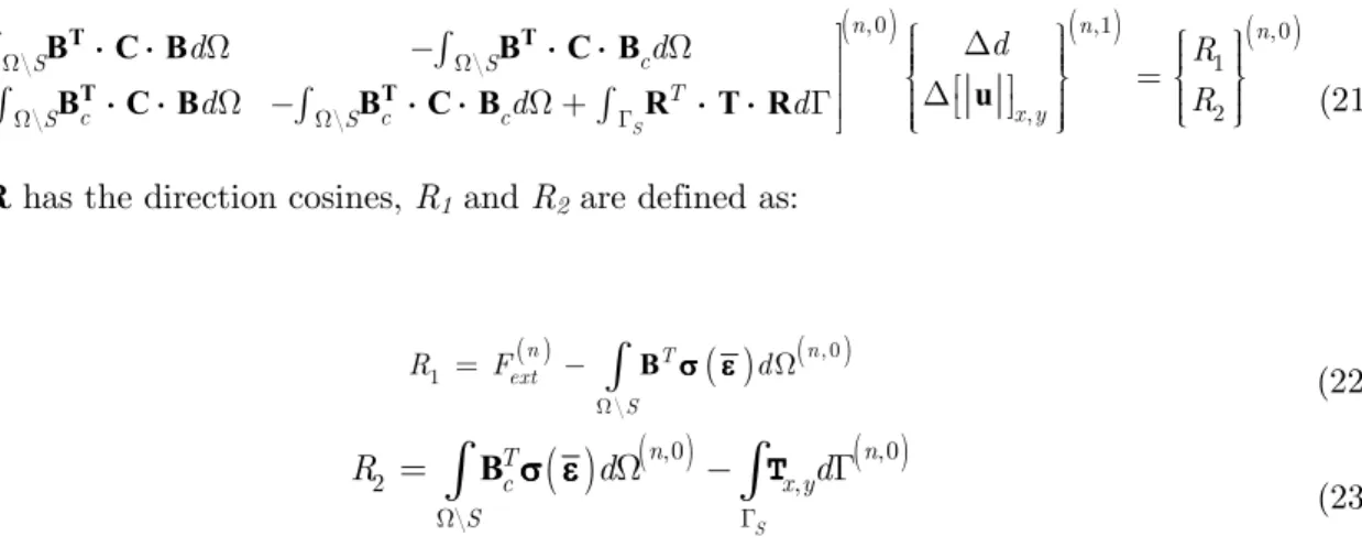
⋅ ⋅ ⋅ ⋅ ⋅ ⋅ (21)
where R has the direction cosines, and are defined as:
( )
( )
( )= −
∫
σ εσ εσ εσ ε (22)( )
( )
( )
Γ
=
∫
σ εσ εσ εσ ε −∫
Γ(23)
To reduce the size of the system given in Eq. (21), the additional degrees of freedom, Δ[|u|], may be condensed. In Eq. (22), means the equilibrium between the external and the internal forces
in the domain , whereas , in Eq. (23), the equilibrium between the forces in the domain
and forces in the discontinuity
Γ
. Tractions at the discontinuity are:=
∫
σσσσ(24)
which expressed in the local system becomes
=
∫
σσσσ(25)
The definitions of the traction vector in Eqs. (24) and (25) are dependent on the discontinuity area, , and the direction cosines to the normal vector n, as shown in Figure 2.
Figure 2: Finite element: a) discontinuity area and b) displacement jumps.
The FEED, given in eq. (21), were implemented in the finite element analysis program (FEAP), developed by Taylor (2008). These FEED capture a discontinuity surface at their geometric cen tre, which is placed perpendicular to the major principal stress direction. The discontinuity sur
x z
y
1
7 4
a)
6
5 8 2
1 4
3
b)
5 8
2
[ ] [ ]
[ ] 3
7
Latin American Journal of Solids and Structures 12 (2015) 2539 2561 faces of the surrounding elements are not aligned as Sancho (2007) did for 2D problems. Although there are formulations which consider linear displacement jumps inside the element such as Alfaiate (2003) and Contrafatto (2012), the displacement jump is constant into these FEED. It is important to say that these elements do not have problems of spurious shear deformations and they satisfied the following requirements: (1) equilibrium, traction conti nuity across the discontinuity interface and (2) kinematics, free relative rigid body motions of the two portions of an element split up by a discontinuity (Juárez Luna and Ayala 2014).
. " ! !#! 2 " (
.*
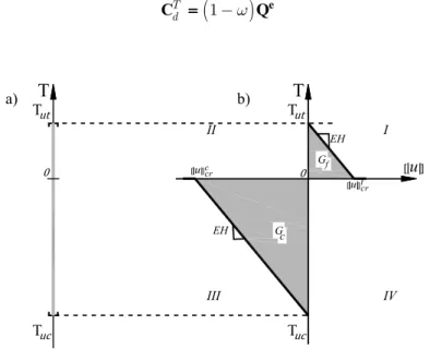
The concrete behaviour was modelled with a discrete damage model, which has different thresh old values under tension and compression, as shown in Figure 3a. This model is equipped with softening after reaching the ultimate tensile strength, T , or the ultimate compressive strength, T , shown in Figure 3b. This model is defined by the following equations:
(
) (
) ( )
(
)
( ) ( )( )
! " # ! ! $ φ α α α φφ α ω φ α
ω
ω ω
α λ α α
∂ ∂ ∂ ∂ = = − = − = − ∈ −∞ = = ∈ ɺ ⋅ ⋅ ⋅ ⋅ ⋅ ⋅ ⋅ ⋅ = ⋅ ⋅ == ⋅⋅ ⋅⋅ = ⋅ ⋅ = ⋅ = ⋅ = ⋅ = ⋅
( )
( )
"% ! "
& ' !
" " "
τ τ
α α α
λ λ λ
′ ∞ = − = = = = ≤ ≤ ≥ = = ɺ ɺ ɺ − −− − − −− − ⋅⋅⋅⋅ ⋅⋅⋅⋅ (26)
whereφ is the discrete free energy density, is the traction vector. The damage variableω is de
fined in terms of the hardening/softening variable ɺ, which is dependent on the harden ing/softening parameter. The damage multiplier λ determines the loading unloading conditions, the function , , bounds the elastic domain defining the damage surface in the tractions space. The tangent constitutive equation, in terms of rates from the model in Eq. (26), is:
ɺ ==== ⋅⋅⋅⋅ ɺ
(27)
where is the tangent constitutive operator, relating the traction and the displacement jump of the nonlinear loading interval, which is defined by
(
)
((
)
α α
ω −
Latin American Journal of Solids and Structures 12 (2015) 2539 2561 and for the elastic loading and unloading interval ( ɺ = and
ω
ɺ
=
):(
−ω)
= == =
(29)
Figure 3:1D discrete damage model with softening: a) elastic space and b) traction displacement jump curve.
This constitutive model considers a material fictitious interpenetration, [|u|]c, when T is over come. Because of the energy dissipation in compression takes place over a surface, rather than within a volume, the use of a fictitious interpenetration instead of a strain is justified (Carpinteri . 2010). In this model, it is assumed that both post peak regimes, tension and compression, have decreasing functions with the same slope, as ca be seen in Figure 3b.
The area under the traction versus jump displacement curve represents the fracture energy density, , in the first quadrant of Figure 3b, :
1
T
2
=
(30)where [|u|] is the critical value of the crack opening, which is given by:
T
= −
(31)Substituting Eq. (31) into Eq. (30) and solving for , the slope of the decreasing function under tension is given by:
2
T
1
2
= −
(32)Considering that the area under the compression versus the fictitious jump interpenetration dis placement curve represents the crushing energy density, , in the third quadrant of Figure 3b, then
Τ
Τut
a)
0
b)
0
Τuc Τuc
Latin American Journal of Solids and Structures 12 (2015) 2539 2561
1
T
2
=
(33)The fictitious critical value of interpenetration can be computed as:
T
= −
(34)Substituting Eq. (34) into Eq. (33), then:
2
T
1
2
= −
(35)As the slope of the decreasing function under tension is the same under compression, Eq. (32) is substituted into Eq. (35):
2
2
T
T
=
(36)If n= T / T in Eq.(36), is given by:
=
2(37)
This equation provides a relationship between the crushing and the fracture energy densities.
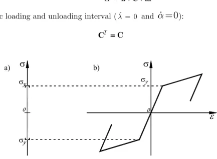
.*-A 1D rate independent plasticity model with isotropic hardening was used for modelling the steel reinforcement. This model has the same threshold value in tension and compression, as shown in Figure 4a; the hardening of the steel reinforcement, after reaching the yield stress σy, was consid
ered with an idealized bilinear function as shown in Figure 4b. The plasticity model is defined by the following equations:
( )
( )
(
)
( )
( )
( )
( )
( )
( )
( )
)*! ! "
# ! ! $ + ! % ! σ σ α
α λ σ λ α
λ α σ α ∂Ψ ∂ ∂ ∂
Ψ = + Ψ
= − = ∂ = ∈ ∞ = = − = ∂Ψ = → = ∂ ′ = → ɺ εεεε
ε ε ε
ε ε ε
ε ε ε
ε ε ε
σ = ε ε
σ =σ = εε εε
σ = ε ε
εεεε
σ σ σ σ
σ σ σ σ
σ σ σ σ
σ σ σ σ
ε ε
εε εε
ε ε
ε ε
ε ε
ε ε
ε ε
( )
( )
& ' !
" " "
α σ
α
λ λ λ
∂ Ψ ′
= =
∂
≤ ɺ≥ ɺ = ɺ=
εεεε
(38)
Latin American Journal of Solids and Structures 12 (2015) 2539 2561
ditions, the function σ,σy , bounds the elastic domain defining the plastic surface in the stress
space. The tangent constitutive equation, in terms of rates from the model in Eq. (38), is:
ɺ ɺ ==== : ε: ε: ε: ε σ
(39)
where is the tangent constitutive operator, relating the stresses and the strain of the nonlinear loading interval, which is defined by
+
⊗ :
⊗⊗ ::
⊗ :
= −
== −−
= −
(40)
and for the elastic loading and unloading interval (λɺ = and
α
ɺ
=
):= == =
(41)
Figure 4:1D rate independent plasticity model with isotropic hardening:
a) elastic space and b) stress strain curve.
4 # ,( 5, 6(
In the presented examples, the reinforcement was meshed with 3D linear finite elements with two nodes, which have three degrees of freedom each. The constitutive behaviour of the steel rein forcement was modelled with a plasticity model with hardening. The steel elements were placed on the edges of the solid elements, coupling the degree of freedom of both kinds of elements. Per fect bond between steel bars and concrete was assumed, as the failure of this type of slabs occurs mainly on flexure without evidence of debonding.
4* 7
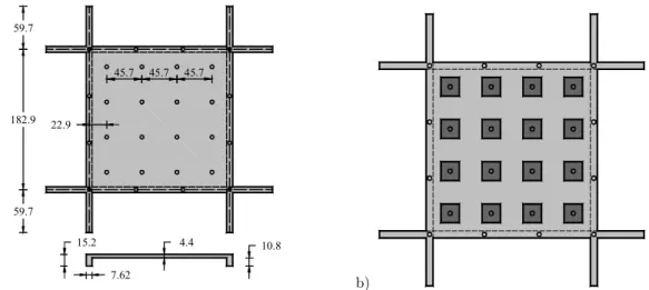
The FEED and the constitutive models were validated by the numerical modelling of the experi mental results reported by Girolami (1970). The test specimen, shown in Figure 5a, is a square slab of sides 1.829 m long and a thickness 0.044 m, which was simple supported at its cor
ε
σ
σya)
σy
σy 0
b)
Latin American Journal of Solids and Structures 12 (2015) 2539 2561 ners. The top and bottom reinforcement used in the slab consisted of 3.66 mm diameter steel bars cut from No.7 gage wire, which were spaced 10.954 cm in both orthogonal directions, as shown in Figure 6a. Also, the stirrups were bent from the No.7 gage steel wire as shown in
Figure 6b. The vertical loads were applied at the top of the slab using four jacks with loading trees distributed to 16 load plates, as shown in Figure 5b. The mechanical properties of the con crete are: Young´s modulus Ec=19.90 GPa, Poisson ratio υ=0.2, ultimate tensile strength
σtu=3.1026 MPa, ultimate compressive strength σuc=31.026 MPa and fracture energy density
Gf=0.098 N/mm. The mechanical properties of the reinforcing steel are: Young´s modulus
Es=206 GPa, Poisson ratio υ=0.3, yield stress σy=330.95 MPa and hardening modulus
H=2.871GPa.
a) b)
Figure 5: Experimental test: a) geometry in cm and b) applied loads (adapted from Girolami . 1970).
a) b)
Figure 6: Reinforcement of: a) one quarter of the slab and b) one half
of a beam (adapted from Girolami . 1970). 182.9
45.7 45.7 45.7
22.9 59.7
59.7
15.2
7.62
4.4 10.8
Top
reinforcement #7 [email protected] cm
4#2 0.4826 m
2#2 3#2
#7 [email protected] cm
Bottom reinforcement
57.15 cm 15.24 cm
10#7wire @ 5.08cm 4#2 66.68 cm
7.62cm 10#7 wire @ 6.35cm3#2 7.62 cm
1
5
.2
4
c
m
1
3
.5
4
c
m
1
3
.5
8
c
m
1
1
.7
9
c
m
A
A'
Section A A'
B
B'
7.62 cm
1
3
.5
4
c
m
Section B B'
4#2 4#2
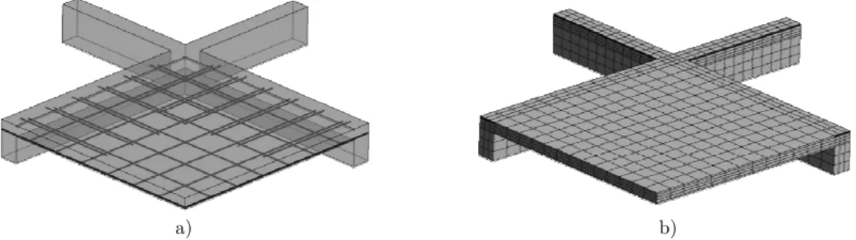
Latin American Journal of Solids and Struct Only one quarter of the slab was modelled, To describe the symmetry conditions at the the degree of freedoms perpendicular to the ment mesh is shown in Figure 7a, whereas Figure 7b.
a)
Figure 7: Meshes: a) steel r
The load displacement at the centre of t curve with FEED shows numerical results
ported by Girolami (1970). In fact, it
ning; however, there is a backward of the sliding of the measurement devices, cons move upwards as the load is applied down ments such as beams, where snapback behav show that the numerical and the experimen puted with the yield line theory. The yield of a slab system by postulating a collapse The moments at the plastic hinge lines ar and the ultimate load is determined using librium (Park and Gamble 2000).
Figure 8: Comparison betw
0.5 0 0 40 80 120 160
Structures 12 (2015) 2539 2561
elled, considering the two axes of symmetry of its geometry at the boundary constraints, no translation was imposed on to the corresponding axes of symmetry. The steel reinforc
ereas the concrete mesh of the slab and beams is shown i
b) steel reinforcement in the slab and b) concrete.
re of the span curves are shown in Figure 8. The compute sults, which are congruent with the experimental curve act, it is observed that both curves are similar at the begi of the displacement. This movement may be attributed to
onsidering that the displacement at the centre would neve downwards; this effect only happens at plain concrete el
behaviour may occur (Carpinteri 1988). It is important t erimental curves are greater than the horizontal curve co yield line theory is a method to estimate the ultimate load lapse mechanism compatible with the boundary condition
es are the ultimate moments of resistance of the section using the principle of virtual work or the equations of equ
n between experimental and numerical results.
3.0
Embedded discontinuity Girolami (1970)
1.0 1.5 2.0 2.5
Yield line theory
ometry. osed on inforce
own in
omputed rve re begin ed to a d never ete ele tant to
com ate load
Latin American Journal of Solids and Structures 12 (2015) 2539 2561 Cracking initiated at the corners on the top surface, growing along the edges to the centre as shown in Figure 9a; on the bottom surface, cracking occurs at the centre, growing to the corner as shown in Figure 9b. The crack patterns at both, top and bottom surfaces, are congruent with the
experimental results reported by Girolami (1970).
(a)
(b)
Figure 9: Cracking propagation on the: a) top and b) bottom surface.
4*-Other two slabs were also analysed, a 4m square slab and a 2m width by 4m length rectangular slab respectively shown in Figure 10; both of them were 10 cm thick and subjected to an increas ing uniform distributed load. Two boundary conditions were considered along their edges: simply supported and clamped. The reinforcement used in the slabs consisted of 3/8 in diameter steel bars, which were spaced 20 cm in both orthogonal directions, as shown respectively in Figures 11 and 12. The mechanical properties of the concrete are: Young's modulus Ec=14710 MPa, Poisson
ratio ν=0.2, ultimate tensile strength σtu=2.86 MPa, ultimate compressive strength σcu=28.63
MPa, fracture energy density Gf=0.098 N/mm. The mechanical properties of the steel reinforce
Latin American Journal of Solids and Structures 12 (2015) 2539 2561
area A=0.71 cm2 and hardening modulus H=2.871 GPa. Like the previous example, the two axes
or symmetry were considered, so only a quarter of the slab was modelled, as shown in Figure 13, which reduces the time consuming of the computational calculation.
Figure 10: Geometry of slabs: a) square and b) rectangular.
(a) (b) (c)
Figure 11: Steel reinforcement of the square slab: a) 3D view, b) first quadrant
with top reinforcement and b) first quadrant with bottom reinforcement.
(a) (b) (c)
Figure 12: Steel reinforcement of the square slab: a) 3D view, b) first quadrant
with top reinforcement and b) first quadrant with bottom reinforcement. 4m
4m
2m
Latin American Jour
(a)
Figure 13: Mesh of slabs: a)
The distributed load . displacement curves at t tively shown in Figure 14. Here, it may be observ clamped slabs are approximately five times great at the displacements of 2.5 and 0.5 cm, respectiv supported slabs, the ultimate load computed wit computed with FEED; on the contrary, for clamp yield line theory is lower than the load compute effect is attributed to the steel reinforcement plac stress before the steel reinforcement placed at the is assumed that every bar instantly reaches the yi
(a)
Figure 14: Distributed load vs. displacement
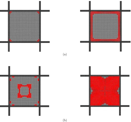
In the clamped square slab, cracking simultaneou growing to the centre until a ring is formed, as sh face, cracking paths form a kind of cross, growin Figure 15b. In the simple supported condition, crac on the bottom surface, growing as shown in Figur corners, growing to the centre, as shown in Figure
Yield line theory
0.5 0 0 20
Clamped Simple supported
100
1.0 1.5 2.0 2.5
40 60 80
n Journal of Solids and Structures 12 (2015) 2539 2561
(b) bs: a) square and b) rectangular.
at the centre of the spans of both slabs are respec observed that the intensity of the distributed load on greater than the intensity on simple supported slabs pectively. Additionally, it is observed that, for simple d with the yield line theory is greater than the load clamped slabs, the ultimate load computed with the omputed with FEED. In simple supported slabs, this placed at the centre of the span reaches the yield at the edges does; whereas in the yield line theory, it the yield stress.
(b)
ement curves in slab: a) square and b) rectangular.
aneously initiated along the edges on the top surface, , as shown in Figure 15a, whereas on the bottom sur growing to the corners and to the edges, as shown in
on, cracking initiated at the corners and at the centre Figure 16b, whereas on top surface, it initiated at the
igure 16a.
Clamped Simple supported Yield line theory
0.1 0 0 20 100
0.2 0.3 0.4 0.5
Latin American Journal of Solids and Structures 12 (2015) 2539 2561
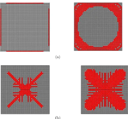
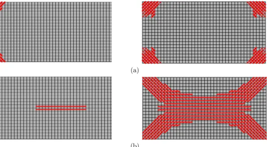
In the clamped rectangular slab, cracking simultaneously initiated along its long edges on the top surface. Then, cracking appeared along its short edges, growing to the centre until a ring is formed as shown in Figure 17a. On the bottom surface, cracking initiated along a strip at the centre of the span, parallel to the long edges, growing to the corners and to the edges, as shown in Figure 17b. In the simple supported rectangular slab, cracking initiated along a strip at the centre on the bottom surface, parallel to the long edges as shown in Figure 18b; some cracks ap peared at the corners on the top surface, as shown in Figure 18a. In general, the cracking paths on the bottom surfaces of the corresponding studied slabs were similar to the paths proposed by the classical yield line theory as well as the experimental results reported by Bach and Graf (1915).
(a)
(b)
Figure 15: Cracking propagation of a clamped square slab on the: a) top and b) bottom surfaces.
Latin American Journal of Solids and Structures 12 (2015) 2539 2561
(b)
Figure 16: Cracking propagation of a simple supported square slab on the: a) top and b) bottom surfaces.
(a)
(b)
Figure 17: Cracking propagation of a clamped rectangular slab on the: a) top and b) bottom surfaces.
(a)
(b)
Latin American Journal of Solids and Structures 12 (2015) 2539 2561
To know if the steel reinforcement yields, the yield strain, εy= σy/Es=0.0021, was compared with
the strains of the steel bars placed perpendicular to the central and edge strips of the slabs, , perpendicular to strips 0 A, 0 a, 0 B, A C, a c and b c, respectively, as shown in Figure 10. The strains of the steel bars were only computed in half of the strips as they are symmetric.
In the clamped square slab, only the central reinforcing top steel bars placed perpendicular to the edge strip yielded as shown in
Figure 19b, while the other bars remained linear elastic as shown in
Figure 19a. This result is congruent with the occurrence of cracking, which simultaneously initiated along the edges on the top surface. On the contrary, in the simple supported square slab, only the central reinforcing bottom steel bars placed perpendicular to the central strip yielded as shown in
Figure 20a, while the other steel bars remained linear elastic as shown in
Figure 20b. This result is also congruent with the occurrence of cracking, which initiated at the centre on the bottom surface.
In the clamped rectangular slab, only the central reinforcing top steel bars placed perpendicu lar to the long edge strip yielded, strip b c, as shown in Figure 21c, while the other bars remained linear elastic as shown in Figure 21a, b and d. This result is congruent with the occurrence of cracking, which simultaneously initiated along the long edges on the top surface. On the contrary, in the simple supported rectangular slab, only the central reinforcing bottom steel bars placed perpendicular to the long central strip yielded, strip 0 a as shown in Figure 22a, while the other bars remained linear elastic as shown in Figure 22b, c and d. This result is also congruent with the occurrence of cracking, which initiated at the centre on the bottom surface.
(a) (b)
Figure 19: Strains in the reinforcing steel bars of the clamped square slab
placed perpendicular to the: a) central strip 0 A and b) edge strip B C. 0.0025
0.0020 0.0015 0.0010 0.0005 0.0000 0.0005 0.0010 0.0015 0.0020 0.0025
0 50 100 150 200
εεεε
Bottom steel Top steel εy
εy
0.0030 0.0020 0.0010 0.0000 0.0010 0.0020 0.0030 0.0040 0.0050
0 50 100 150 200
εεεε
Bottom steel Top steel εy
Latin American Journal of Solids and Structures 12 (2015) 2539 2561
(a) (b)
Figure 20: Strains in the reinforcing steel bars of a simple supported slab
placed perpendicular to the: a) central strip 0 A and b) edge strip B C.
(a) (b)
(c) (d)
Figure 21: Strains in the reinforcing steel bars of a clamped rectangular slab placed perpendicular to the: a)
central strip 0 a, b) central strip 0 b, c) edge strip b c and c) edge strip a c. 0.0030 0.0020 0.0010 0.0000 0.0010 0.0020 0.0030 0.0040 0.0050
0 50 100 150 200
εεεε Bottom steel Top steel εy εy 0.0025 0.0020 0.0015 0.0010 0.0005 0.0000 0.0005 0.0010 0.0015 0.0020 0.0025
0 50 100 150 200
εεεε Bottom steel Top steel εy εy 0.0025 0.0020 0.0015 0.0010 0.0005 0.0000 0.0005 0.0010 0.0015 0.0020 0.0025
0 50 100 150 200
εεεε Bottom steel Top steel εy εy 0.0025 0.0020 0.0015 0.0010 0.0005 0.0000 0.0005 0.0010 0.0015 0.0020 0.0025
0 20 40 60 80 100
εεεε Bottom steel Top steel εy εy 0.0030 0.0020 0.0010 0.0000 0.0010 0.0020 0.0030 0.0040
0 50 100 150 200
εεεε Top steel Bottom steel 0.0025 0.0020 0.0015 0.0010 0.0005 0.0000 0.0005 0.0010 0.0015 0.0020 0.0025
0 20 40 60 80 100
εεεε
Top steel Bottom steel εy
Latin American Journal of Solids and Structures 12 (2015) 2539 2561
(a) (b)
(c) (d)
Figure 22: Strains in the reinforcing steel bars of a simple supported rectangular slab placed perpendicular
to the: a) central strip 0 a, b) central strip 0 b, c) edge strip b c and c) edge strip a c.
8 " (# "
The FEED with a discrete damage model were used for modelling concrete slabs under vertical load, involving their crack pattern and the load displacement capacity curve. The discrete dam age model considers a constitutive behaviour equipped with softening for the concrete elements limited for a damage surface, whereas for the reinforced concreted elements, a 1D rate independ ent plasticity model was assigned to the reinforcement, which take into account the hardening of the steel as isotropic.
The coupling of solid FEED and bar elements was validated with experimental results re ported in the literature. Although the experimental curve shows a recovery of the displacement, it is considered that it was an effect of a slipping of the measurement equipment, since under an increasing vertical load it is not possible a recovery of the displacement at the centre of the span.
In clamped slabs, cracking initiated on the top surface at the centre of its edges, growing to the corners until a kind of ring is formed. On the bottom surface, cracking occurred at the centre of the span, propagating to the corners until a cross is formed. Whereas, in simple supported
0.0050 0.0000 0.0050 0.0100 0.0150 0.0200 0.0250
0 50 100 150 200
εεεε Bottom steel Top steel εy εy 0.0025 0.0020 0.0015 0.0010 0.0005 0.0000 0.0005 0.0010 0.0015 0.0020 0.0025
0 20 40 60 80 100
εεεε Bottom steel Top steel εy εy 0.0025 0.0020 0.0015 0.0010 0.0005 0.0000 0.0005 0.0010 0.0015 0.0020 0.0025
0 50 100 150 200
εεεε Bottom steel Top steel εy εy 0.0025 0.0020 0.0015 0.0010 0.0005 0.0000 0.0005 0.0010 0.0015 0.0020 0.0025
0 20 40 60 80 100
εεεε
Bottom steel Top steel εy
Latin American Journal of Solids and Structures 12 (2015) 2539 2561 slabs, cracking initiated at the centre of the span on the bottom surface, propagating to the cor ners until a cross was formed. On the top surface, incipient cracking occurred at the corners.
The ultimate load computed for simple supported slabs with the yield line theory is greater than the load computed with FEED; on the contrary, for clamped slabs, the ultimate load com puted with the yield line theory is lower than the load computed with FEED. In simple supported slabs analysed with FEED, this effect is attributed that the steel reinforcement at the centre of the span reached the yield stress before the steel reinforcement placed at the edges did; whereas with the yield line theory, it is assumed that every bar instantly reaches the yield stress.
In the clamped square slab, the central reinforcing steel bars placed perpendicular to the edges yielded, while in the simple supported square slab the central reinforcing steel bars placed perpendicular to central strip yielded. On the other hand, in the clamped rectangular slab, the reinforcing steel bars placed perpendicular to the long edges yielded, while in the simple sup ported rectangular slab, the reinforcing steel bars placed perpendicular to long central strip yielded. These results were congruent with the places of the slabs where cracking initiated, corre sponding to the places where grater tension stresses occurred.
,
The first author acknowledges the support given by the Universidad Autónoma Metropolitana and the financial support by CONACYT under the agreement number I010/176/2012, in the context of the research project: “Analysis and design of concrete slabs”. The third author ac knowledges the sponsorship by the General Directorate of Academic Personnel Affairs of UNAM of the PAPIIT project IN108512.
ABAQUS (2011). Example problems manual, Volumen1: static and dynamic analysis, Version 6.11, E.U.A., p.881. Alfaiate, J., Simone, A., Sluys, L.J. (2003). Non homogeneous displacement jumps in strong embedded discontinui ties, International Journal of Solids and Structures 40 (21): 5799 5817.
ANSYS. (2010). ANSYS User’s Manual version 13.0, ANSYS, Inc., Canonsburg, Pennsylvania, USA.
Bach, C., Graf, O. (1915). Versuche mit allseitig aufliegenden, quadratischen and rechteckigen eisenbetonplatten, Deutscher Ausschuss für Elsenbeton 30, Berlin. (In German)
Carpinteri, A. (1988). Cusp catastrophe interpretation of fracture instability, Journal of the Mechanics and Physics of Solids 37(5): 567 582.
Carpinteri, A., Carrado, M., Paggi M. (2010). An integrated cohesive/overlapping crack model for the analysis of flexural cracking and crushing in RC beams, International Journal of Fracture 161:161 173.
Casadei, P., Parretti, R., Nanni, A., Heinze, T. (2005). In situ load testing of parking garage reinforced concrete slabs: comparison between 24 h and cyclic load testing, ASCE Practice Periodical on Structural Design and Con struction 10(1): 40 48.
Latin American Journal of Solids and Structures 12 (2015) 2539 2561
de Borst, R., Nauta, P. (1985). Non orthogonal cracks in a smeared finite element model, Engineering Computations 2(1): 35 46.
DIANA (2008). DIANA 9.0: Finite Element Analysis User's Manual Release, TNO DIANA BV, Delft, Holanda. Foster, S.J., Bauley, D.G., Burgess, I.W., Plank, R.J. (2004). Experimental behaviour of concrete floor slabs at large displacements, Engineering Structures 26(9): 1231 1247.
Galati, N., Nanni, A., Tumialan, J.G., Ziehl, P.H. (2008). In situ evaluation of two concrete slab systems, I: load determination and loading procedure” ASCE Journal of Performance of Constructed Facilities 22(4): 207 216. Gamble, W.L, Sozen, M.A., Siess, C.P. (1961). An experimental study of a two way floor slab, Structural Research Series No. 211, Department of Civil Engineering, University of Illinois, p. 326.
Gilbert, R.I., Warner, R.F. (1978). Tension stiffening in reinforced concrete slabs. ASCE Journal of the Structural Division 104(12): 1885 1900.
Girolami, A.G., Sozen M.A., Gamble, W.L. (1970). Flexural strength of reinforced concrete slabs with externally applied in plane forces, Report to the Department of Defense, Illinois University, Urbana, Illinois.
Hand, F.D., Pecknold, D.A., Schnobrich, W.C. (1973). Nonlinear analysis of reinforced concrete plates and shells, ASCE Journal of the Structural Division 99(7): 1491 1505.
Hatcher, D.S., Sozen, M.A, Siess, C.P. (1960). An experimental study of a quarter scale reinforced concrete flat slab floor, Structural Research Series No. 200, Department of Civil Engineering, University of Illinois, p. 288.
Hatcher, D.S., Sozen, M.A., Siess C.P. (1961). A study of tests on a flat plate and a flat slab, Structural Research Series No. 217, Department of Civil Engineering, University of Illinois, p. 504.
Hinton, E., Abdel Rahman, H.H., Zienkiewicz, O.C., (1981). Computational strategies for reinforced concrete slab systems, International Association of Bridge and Structural Engineering, Colloquium on Advanced Mechanics of Reinforced Concrete: 303 313.
Jirsa, J.O., Sozen, M.A., Siess, C.P. (1962). An experimental study of a flat slab floor reinforced with welded wire fabric, Structural Research Series No. 248, Department of Civil Engineering, University of Illinois, p. 188.
Jofriet, J.C., McNeice, G.M. (1971). Finite element analysis of RC slabs, ASCE Journal of the Structural Division, 97 (3) 785 806.
Juárez, G., Ayala, G. (2009). Variational formulation of the material failure process in solids by embedded disconti nuities model, Numerical Methods for Partial Differential Equations 25(1): 26 62.
Juárez Luna, G., Ayala, G.A. (2014). Improvement of some features of finite elements with embedded discontinuities, Engineering Fracture Mechanics 118:31 48
Juárez Luna G., Caballero Garatachea O. (2014). Determinación de coeficientes de diseño y trayectorias de agrieta miento de losas aisladas circulares, elípticas y triangulares, Ingeniería Investigación y Tecnología XV(1):103 123. (In spanish)
Kabele, P., Cervenka, V., Cervenka, J. (2010). ATENA Program Documentation. Example Manual, ATENA Engi neering, p. 90.
Kupfer, H.B., Gerstle, K.H. (1973). Behaviour of concrete under biaxial stresses, ASCE Journal of Engineering Me chanics 99 (4): 853 866.
Kwak, H.G., Filippou, F.C. (1990). Finite element analysis of reinforced concrete structures under monotonic loads, Department of Civil Engineering, University of California, Berkeley, California, p. 124.
Lin, C.S., Scordelis, A.C. (1975). Nonlinear analysis of RC shells of general form, ASCE Journal of the Structural Division 101(3): 523 238.
Latin American Journal of Solids and Structures 12 (2015) 2539 2561
Mayes, G.T., Sozen, M.A., Siess, C.P. (1959). Tests on a quarter scale model of a multiple panel reinforced concrete flat plate floor, Structural Research Series No. 181, Department of Civil Engineering, University of Illinois.
Mcneice, A.M. (1967). Elastic plastic bending of plates and slabs by the finite element method, Dissertation, London University.
Oliver, J. (1996). Modelling strong discontinuities in solid mechanics via strain softening constitutive equations, Part 1: Fundamentals, 39(21): 3575 3600. Part 2: Numerical simulation, International Journal for Numerical Methods in Engineering 39(21): 3601 3623.
Park, R., Gamble, W.L. (2000). Reinforced concreted slabs, John Wiley & Sons, second edition.
Rots, J.G. (1988). Computational modeling of concrete fracture, Dissertation, Delft University of Technology, The Netherlands, p.132.
Sancho, J.M., Planas, J., Cendón, D.A., Reyes, E., Gálvez, J.C. (2007). An embedded crack model for finite element analysis of concrete fracture, Engineering Fracture Mechanics 74(1 2): 75 86.
Smadi, M.M., Belakhdar, K.A. (2007). Development of finite element code for analysis of reinforced concrete slabs, Jordan Journal of Civil Engineering 1(2): 202 219.
Taylor, L.R. (2008). A finite element analysis program (FEAP) v8.2, Department of Civil and Environmental Engi neering, University of California at Berkeley, Berkeley, CA.
Vanderbilt, M.D., Sozen, M.A., Siess, C.P. (1961). An experimental study of a reinforced concrete two way floor slab with flexible beams” Structural Research Series No. 228, Department of Civil Engineering, University of Illinois, p. 188.
Wang, Y., Dong, Y., Zhou G. (2013). Nonlinear numerical modeling of two way reinforced concrete slabs subjected to fire, Computers & Structures 119(1): 23 36.
Wells, G.N., Sluys, L.J. (2001). A new method for modelling cohesive cracks using finite elements, International Journal for Numerical Methods in Engineering 50(12): 2667 2682.