Universidade de Lisboa
Faculdade de Ciências
Departamento de Engenharia Geográfica, Energia e Geofísica
Spatially: A Spatial Analysis Web GIS Prototype
System
Alexandra Dias
Projeto
Mestrado em Engenharia Geográfica
2014
Universidade de Lisboa
Faculdade de Ciências
Departamento de Engenharia Geográfica, Energia e Geofísica
Spatially: A Spatial Analysis Web GIS Prototype System
Alexandra Dias
Projeto para obtenção de Grau de Mestre orientado por:
Prof.ª Doutora Cristina Catita (Faculdade de Ciências da Universidade de
Lisboa) e
Prof. Doutor Michael Flaxman (Geodesign Technologies Inc.)
Mestrado em Engenharia Geográfica
i Abstract
Geographic information is increasingly more present in several areas of knowledge, resulting in the fact that around 80% (Zhang et al., 2010) of the databases include spatial information.
Processes of visualization and application of algorithms to spatial data are already common in the daily routine of any internet user.
The accentuated development of information and communication technologies have resulted in the appearance of increasingly more efficient technologies with the capacity of dealing with big data volumes with a geospatial component. Despite the effort over the last years in the development of Open source technologies related with this area, options that do not require the installation of software and that are accessible to a diverse range of publics are still lacking.
In Portugal, Census represent the biggest source of information about population, family, housing available having a defined spatial character and comprehending information with potential interest in a wide range of investigation themes.
As a result of the above, what is proposed in this project is the creation of a platform on the internet that allows the users to perform spatial analysis over their and/or a default data set from Census made available by the platform. The methods to be applied include visualization, spatial autocorrelation analysis and building spatial regression models over a defined dataset. Besides the evident functionality to achieve it is also pretended to gather an overview over the open source technologies available for the construction of a Web Gis (from the database to the geospatial data server and the display and analysis of the mentioned data) as well as their potentialities and limitations at the moment. Finally it is aimed to integrate three elements: an understanding of spatial analysis methods to be applied to geospatial data in areal sections, an exploration of the technologies available for the proposed goals mainly within the Open Source software area and the definition of system architectures according to the proposed objectives.
Key - words: Spatial Analysis, Web Architecture, Open Source, Census, Web-based GIS
ii Sumário
A informação geográfica está cada vez mais presente em diversas áreas de conhecimento, sendo que cerca de 80 % das bases das bases de dados inclui informação espacial. Processos de visualização de informação geográfica e aplicação de algoritmos com componente geográfica são já comuns no dia-a-dia de qualquer utilizador da internet.
O acentuado desenvolvimento das tecnologias de informação e comunicação tem resultado no aparecimento de tecnologias cada vez mais eficientes, e com capacidade de lidar com grandes volumes de dados com componente geoespacial. Apesar dos esforços dos últimos anos no desenvolvimento das tecnologias de código aberto e licença livre (open source) relacionados com esta área, são ainda escassas as opções que não impliquem instalação de software e que sejam acessíveis a diversos públicos.
Os Censos em Portugal representam a maior fonte de informação sobre população, família e habitação disponível, tendo esta um carácter espacial muito definido e compreendendo informação com potencial interesse para diversos tema de investigação. Assim, o que se propõem neste projecto é a criação de um protótipo de plataforma na web que permita ao utilizador fazer análise espacial sobre os seus dados e/ou um conjunto de dados dos censos disponibilizado pela plataforma. Os métodos incluem visualização, análise de autocorrelação espacial e criação de modelos de regressão espacial com base nos dados mencionados. Além da evidente funcionalidade a atingir, pretende-se ainda fazer um levantamento das tecnologias (software e ferramentas) Open
Source disponíveis para a construção de um Web Sig (desde a base de dados, ao sevidor
de dados espaciais e disponibilização e análise dos mesmos), bem como das suas potencialidades e limitações actualmente. Finalmente, pretende-se fazer uma integração de três elementos: uma compreensão dos métodos estatísticos de análise espacial referidos, uma exploração das tecnologias (ao nível de software) Open Source disponíveis para os fins definidos e a definição de estruturas de arquitectura de acordo com a finalidade proposta.
iii Resumo
A informação espacial tem cada vez mais expressão numa sociedade com uma crescente tendência para a tecnologia, sendo inclusivamente referido pela literatura que cerca de oitenta por cento da informação contida em bases de dados corporativas contém uma vertente espacial (Zhang et al., 2010).
A evolução das capacidades computacionais, e a sua passagem para um ambiente virtual tem-se revelado de extremo interesse para a indústria tecnológica com reflexo na utilização de ambientes cloud para o devido efeito em diversas aplicações na internet (Song et al., 2010; She et al,. 2012; Anselin et al., 2004). Associando a estes factores a recente tendência das comunidades tecnológicas para o software de código aberto e licença livre, obtém-se o ambiente perfeito de aprendizagem para um projeto de mestrado.
Este projeto nasce da escassez documentada pela bibliografia (Zhang et al., 2010; She et al., 2012) de ambientes online que permitam fazer análise espacial sobre os dados de forma intuitiva e com instrução de acompanhamento. Propondo-se neste contexto a realização de um protótipo de sistema de SIG na internet com incorporação de funcionalidades de análise espacial.
Os objectos definidos para este projeto compreendem:
A compreensão e exploração de métodos e aplicações de análise espacial;
O desenho da arquitectura de um protótipo de um sistema Web SIG;
A exploração das opções software de código aberto disponíveis para a disponibilização de serviços SIG na internet;
O desenho e o preenchimento de uma base de dados espacial;
A produção de um protótipo de website de acordo com as conclusões dos tópicos anteriores;
A exploração e implementação de funcionalidades de análise espacial num
website com ferramentas interactivas;
A implementação de um sistema de relatório de forma a produzir um documento PDF com os resultados dos métodos de análise espacial aplicados.
Com vista a permitir que esta plataforma tenha aplicabilidade não só entre a comunidade científica, mas também entre utilizadores comuns, disponibiliza-se, além da opção de utilização dos próprios dados através da transferência do ficheiro de dados
iv próprios, a opção de definir de entre um dos conjuntos de dados disponibilizados (dados referentes ao Censos 2011 disponibilizados pelo Instituto Nacional de Estatística (INE)).
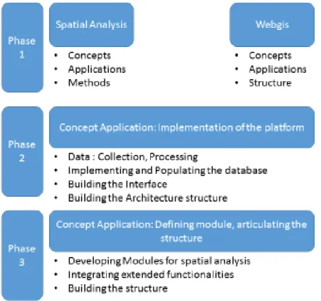
O projeto está definido em três fases principais (a consultar na Figura 1 do referido documento) que consistem sucintamente em:
- Fundamentação teórica - compreendendo conceitos, aplicações e métodos tanto de análise espacial como de Web SIG;
- Implementação da plataforma – abarcando a aplicação dos conceitos definidos na fase anterior e incluindo grande parte do processo de implementação da plataforma (desde a colecção de dados até à implementação da base de dados e posteriormente construção da aplicação per se);
- Definição de módulos, articulação da estrutura – onde se integram todos os componentes integrantes da plataforma com a sua total funcionalidade. Esta fase inclui o desenvolvimento dos módulos de análise espacial, bem como de funcionalidades que estendem o protótipo base, tal como a funcionalidade de
login e os formulários de interacção entre o servidor e o cliente.
A análise espacial é uma área com interesse em inúmeras aplicações amplamente referidas na bibliografia (Beale et al., 2010; Rey, 2007; Druck et al., 2004). Ciências Sociais, Biologia, Criminologia, Epidemiologia (...) são algumas das áreas que fazem extensivo uso da análise espacial, sem terem, contudo, formação específica para lidar com dados com uma componente espacial.
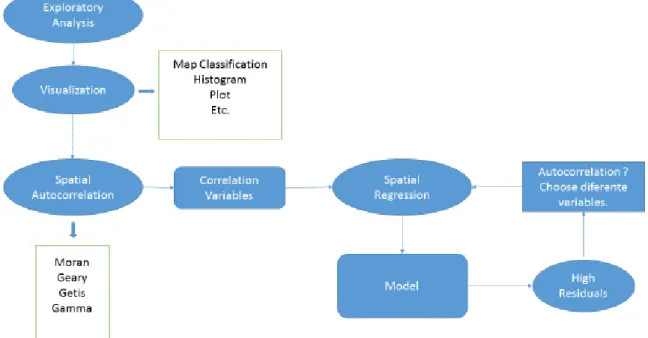
Assim, são apresentadas três etapas de análise espacial (a implementar no protótipo) que contemplam a visualização dos dados, a análise exploratória dos mesmo (englobando a análise de autocorrelação espacial) e a regressão espacial.
Estes três conjuntos de métodos estão encadeados num processo cíclico, e requerem uma interpretação informada. Um dos factores contemplados no capítulo 2 do documento está relacionado com a conceptualização do problema em causa, que é um dos maiores desafios do processo de análise espacial.
A definição da estrutura do protótipo é definida de acordo com (Mao 2005). Neste sentido definem-se os quatro componentes essenciais da arquitectura do protótipo do sistema de Web SIG : Base de Dados, Servidor, Web Framework e Linguagens de programação associadas (tanto no lado do servidor como do cliente).
v Numa comparação superficial sobre o software de código aberto disponível, com uma forte base num estudo de Ballatore (Ballatore et al. 2011) que propõem uma comparação com base nos parâmetros definidos pelo utilizador. Os projetos open source considerados neste documento têm já como pré-requisito o facto de serem direccionados a dados com componentes geospaciais. Desta investigação resulta a definição do
software e das tecnologias a utilizar na implementação do protótipo:
PostgreSQL (com extenção PostGIS), GeoServer, Django (extenção GeoDjango), Python – como linguagem de programação no lado do servidor, e Javascript, HTML,
css como linguagens de scripting do lado do cliente.
A implementação do protótipo é feita com base em dados da Carta Administrativa Oficial Portuguesa (CAOP) do continente disponibilizada pelo INE, sendo os dados processados de acordo com os requisitos do sistema e agrupados em áreas de diferentes dimensões (freguesias, concelhos e distritos), com fim a serem inseridos na base de dados. As operações às quais a informação geográfica foi sujeita podem ser consultados de forma esquemática na página 46, sendo que o esquema final em Modelo de dados OMT-G de bases de dados geográfica na figura 20.
O interface do utilizador é também definido nesta segunda fase do processo onde se apresenta ferramentas para tal efeito. Este tópico, é no entanto considerado menos relevante no âmbito do projeto, e sendo consequentemente abordado de forma mais superficial.
A terceira fase do projeto compreende o desenvolvimento dos módulos em Python, integrando uma lista de bibliotecas da mesma linguagem, cuja estrutura e dependências é apresentada na figura 15. No capítulo 5 definem-se os módulos a construir e as funcionalidades a implementar nos mesmos, definindo-se ainda as variáveis de entrada e saída de cada função. Funcionalidades como o login e os formulários são também documentadas nesta etapa, que resulta na implementação do protótipo de sistema final com todas as funcionalidades propostas.
Os relatórios produzidos são finalmente apresentados, sendo os resultados organizados num ficheiro PDF com informações referentes aos dados e às análises efectuadas. O projeto apresentado, apesar de contemplar algumas áreas de elevado interesse: tanto no meio académico como na indústria, teve bastantes limitações relacionadas maioritariamente com assuntos de carácter técnico. Dentre os quais se destacam as dificuldades de instalação de bibliotecas, os obstáculos na definição da arquitectura de forma a servir a informação online e os recursos em termos de servidor. Durante o
vi projeto, foram várias as abordagens relativamente a estes assuntos (especialmente no que toca à configuração do ambiente Python e o serviço dos dados), que foram sendo ultrapassados recorrendo a servidores externos.
De uma maneira geral, o projeto atinge os objectivos a que se propunha, tendo no entanto algumas limitações em termos de funcionalidades e uma generosa lista de trabalho proposto que no âmbito da disciplina não faria sentido desenvolver. As potencialidades computacionais deste tipo de projeto podem ser variadas, conforme os recursos disponíveis no servidor, sendo inclusivamente proposta a passagem do ambiente para um servidor com mais recursos, e mais flexível que permita uma interacção entre utilizadores numa comunidade de dados espaciais com capacidade de análise e investigação sobre dados de outros cientistas.
Em termos de software opensource, conclui-se que a sua utilização depende em grande parte da utilização pretendida, e que apesar da considerável documentação, problemas técnicos implicam necessariamente mais tempo do que num caso de software comercial em que há a possibilidade de apoio técnico. No entanto, e no caso deste projeto, a sua flexibilidade permite a execução de funcionalidades que dificilmente seriam implementadas com código fechado. Revelando-se particularmente interessante devido à flexibilidade de implementação e tendo, para o efeito requerido, sido sobejamente eficiente.
vii
Acknowledgements
No one is an Island, and we are all a sum of everything we choose to absorb from the people who pass us by.
With this declaration I must be thankful to my parents, the most important people in my life who made me the complete person I am today. I am also very thankful for my siblings: friends, accomplices and companions who are so very present in every aspect of my life and to whom I look up to for many reasons.
My grandparents, whose lessons and ideals will always accompany me as a great part of my character. To my friends and family, whose presence and support made this journey a lot easier, especially João for being so comprehensive and supportive.
I am especially thankful to Prof. Dr. Cristina Catita, for giving me the space to grow while providing support, orientating me in the right direction and for teaching me that most of the times the journey will teach us far more than the destination. To Prof. Dr. Michael Flaxman, for giving me such an amazing opportunity and for the orientation regarding technologies and to Eng. Rita Semedo, my internship coordinator, for being so flexible and comprehensive during the thesis process.
Furthermore, I dedicate this work to my grandfather, whose kindness, strong character and ethics will always be very present in my journey.
viii
List of Figures
Figure 1 : Schematized summary of the phases of the present project. ... 4 Figure 2 : Summary of the topics covered in each chapter of the present document. ... 7 Figure 3 : The characteristics of geospatial data. a. Location, attribute and time, related with the elementary questions Where, What and When, b. the object view, c. detailed characteristics of data components (Source : (Kraak & Ormeling, 2010), p. 4) ... 9 Figure 4 : Discrete and continuous space representations. (Source:(Haining 2004), p. 45) ... 11 Figure 5 : Conceptualization and Representation, the relationship between the Real World and the Data Matrix. (Source: Haining, 2004) ... 12 Figure 6 : Spatial Regression Model Equation Explanation with example. (Source: (Scott, 2009)) ... 23 Figure 7 : Illustration of spatial relationship according to the explanatory variables signal. (Source: (Scott, 2009)) ... 25 Figure 8 : Spatial Analysis functionalities to be implemented. Schematized structure. 29 Figure 9 : Schema of a Web GIS application (Source: (Amrita, 2012)). ... 33 Figure 10 : Basic DBMS schema (Source: (Gillenson, 2011)). ... 35 Figure 11 : Spatial database management systems (Source: (Ballatore et al., 2011) p.17) ... 36 Figure 12 : Comparison between sever web mapping servers and spatial libraries
(Source: (Ballatore et al., 2011), p. 16) ... 37 Figure 13 : Interaction between JavaScript, CSS and HTML in a modern Web Site or Application (Source: (MASS MEDIA GROUP LTD., 2011)) ... 38 Figure 14 : Comparison of Javascript libraries and mapping services for map
ix Figure 15 : Illustrating schema of the Python libraries to be applied and required
dependencies. ... 40
Figure 16 : MTV Schema: necessary files and core structure of a MTV model. ... 41
Figure 17 : GeoDjango Structure, including basic libraries, available databases, implemented standards and displaying format (Source:(Springmeyer, 2009)). ... 42
Figure 18 : Workflow of the prototype WebGIS system... 43
Figure 19 : Data processing diagram, including all the datasets used and geoprocessing operations applied. ... 46
Figure 20 : Classes and transformations Diagram ... 48
Figure 21 : Geodjango structure: Main core components and Required Libraries. ... 49
Figure 22 : Spatially: Web GIS Prototype System - Home Page ... 50
Figure 23 : Spatially: Web GIS Prototype System - Instructions Page ... 51
Figure 24 : Spatially: Web GIS Prototype System: About Page ... 51
Figure 25 : Spatially Web GIS Prototype System: Spatial Analysis Page. ... 52
Figure 26 : Django Project File Structure - Spatially Example ... 53
Figure 27 : Django Application File Structure - Spatially: Sa (spatial analysis). ... 53
Figure 28 : Spatially: The Prototype System Structure. ... 54
Figure 29 : Spatially: Web GIS Prototype System: Django Admin Web Page ... 57
Figure 30 : Spatially Module Structure ... 60
Figure 31 : Histogram: Rate of unemployed people looking for their first jobs. ... 60
Figure 32 : Map Classification: Quantiles, Equal Intervals and Fisher Jenks Methods (correspondently) – projected in WGS84. ... 61
Figure 33 : Moran's I empirical distribution (expected distribution in blue and actual value in red). ... 62
x Figure 34 : Permutations of Moran's I index in comparison with the normal distribution
line. ... 62
Figure 35 : Empirical distribution and value of Geary's C index ... 62
Figure 36 : Lisa Cluster Map for rates of ... 63
Figure 37 : Ordinary Least Square Output Example. ... 65
Figure 38 : Error Model Output Example. ... 66
Figure 39 : Spatial Lag Output Example. ... 67
List of tables
Table 1 – Dimensions of data quality in relation to stages of spatial analysis. (Source: (Haining, 2004) p. 178 ) ... 14Table 2 – Summary of graphical methods for data visualization. (Source: (Haining,2004), p. 194) ... 17
Table 3 - Normal distibution , z-score, p-value and confidence level (Source:(ESRI, 2013)). ... 23
Table 4 – User Interface pages, descriptions and technologies applied. ... 50
xi
Acronyms
GIS – Geographic Information Systems SDI – Spatial Data Infrastructure OS – Open Source
EDA – Exploratory Data Analysis
ESDA – Exploratory Spatial Data Analysis
ESRI – Environmental Systems Research Institute MAUP – Modifiable Areal Unit Problem
OLS – Ordinary Least Squares
DBMS – Database Management Software SQL – Structures Query Language
PK – Primary Key
OGC – Open Geospatial Consortium HTML – Hypertext Markup Language CSS – Cascading Style Sheet
GEOS – Geometry Engine Open Source GDAL – Geospatial Data Abstraction Library WAF – Web Application Framework
MVC – Model - View - Controller URL – Uniform Resource Locator
CAOP – Carta Administrativa Oficial de Portugal (Portugal’s Oficial Administrative Map)
EPSG – European Petroleum Survey Group
ETRS89 – European Terrestrial Reference System 1989 GRS – Geodetic Reference System
xii OGP - (International Association of) Oil & Gas Producers
IGP – Instituto Geográfico Português ( Portuguese Geographical Institute INE – Instituto Nacional de Estatítica ( National Statistics Institute) GIF- Graphics Interchange Format
JPEG – Joint Photographic Experts Group IT – Information Technology
OSGEO4W – Open Source Geospatial For Windows CI – Cyber Infrastructure
xiii
Index
1. Introduction ... 1 1.1. Research Objectives ... 1 1.2. Problem Statement ... 2 1.3. Methodology ... 3 1.4. Research Significance... 4 1.5. Thesis Structure ... 62. GIS applications for Spatial Analysis ... 9
2.1. Thesis Concepts ... 9
2.1.1. Spatial Data ... 9
2.1.2. Spatial analysis ... 10
2.1.3. Conceptualization and data proprieties ... 10
2.1.4. Data Quality ... 13
2.1.5. Areal Data Problems ... 14
2.2. Spatial Analysis Methods ... 15
2.2.1. Data Visualization ... 16
2.2.2. Weights ... 17
2.2.3. Exploratory spatial data analysis ... 18
2.2.4. Spatial Regression ... 23
2.3. Application of spatial analysis ... 28
2.4. Chapter Summary ... 28
3.Web-Based GIS ... 31
xiv
3.2. State of the art of Web-Based GIS architecture ... 33
3.3. Overview of Web-Based GIS Technologies ... 35
3.3.1. Database ... 35
3.3.2. Server ... 37
3.3.3. Hypertext Markup Language (HTML) ... 37
3.3.4. Cascading Style Sheets (CSS) ... 38
3.3.5. Javascript ... 38
3.3.6. Python Libraries ... 39
3.3.7. Web framework ... 40
3.4. Chapter Summary ... 42
4. Prototype and System Implementation ... 43
4.1. System requirement Analysis ... 43
4.1.1. Prototype implementation ... 43
4.1.2. Data Collection ... 43
4.1.3. Spatial data processing ... 44
4.1.4. Spatial Database design ... 47
4.1.5. Website Setup ... 49
4.1.6. User Interface Development ... 49
4.1.7. Website structure ... 52
4.2. Implementation obstacles ... 54
4.3. Chapter Summary ... 55
5. System Enhancement and Spatial Analysis Implementation ... 57
5.1. Prototype System Enhancement ... 57
5.1.1. Login ... 57
xv
5.2. Spatial Analysis Modules ... 58
5.2.1. Tools ... 58
5.2.2. Implemented Modules ... 58
5.3. Report implementation ... 68
5.4. Chapter Summary ... 68
6. Conclusions and Recommendations ... 69
6.1. Summary of Research ... 69
6.2. Conclusions ... 70
6.3. Conclusions regarding the followed methodology ... 72
6.4. Research contributions ... 73
6.5. Limitations ... 74
6.6. Recommendations for future work ... 76
References ... 79
Attachments ... 87
1. Available DataSources for Portuguese data ... 87
2. Statistical methods applied: Inputs and Outputs ... 91
3. Instruction Section ... 99
xvi
“The application of GIS is limited only by the imagination of those who use it”.
1
1. Introduction
1.1. Research Objectives
Geographic Information Systems (GIS) have added many interesting options to the applications of Spatial Information. Data collection, storage, visualization, manipulation and analysis have been becoming less complex tasks throughout the years with the appearance of more developed and complex data infrastructures that propose themselves to accomplish the computational effort that all these processes involve.
This project has the objective of producing a simple tool for common users and scientists to analyze geospatial data, considering that the common user is not very familiar with this type of data nor with the spatial analysis functionalities.
The proposition consists in building a web infrastructure capable of receiving, analyzing and reporting on a specific input dataset or on a dataset collection made available by the platform, and according to a set of methods of spatial analysis defined by the user. This kind of platform often receives the name of Spatial Data Infrastructure (SDI) and it is a data infrastructure that implements a framework of geographic data, metadata, users and tools that are interactively connected in order to use spatial data in an efficient and flexible way (Pascaul et al., 2012). According to Scholten et al. (2009), an SDI is a coordinated series of agreements on technology standards, institutional arrangements, and policies that enable the discovery and use of geospatial information by users and for purposes other than those it was created for.
More specifically this infrastructure aims at two specific users: Scientists who, being familiar with this type of data, are not very comfortable with the process of analyzing it, or the common user who will have a dataset available with statistical data of Portugal which can be explored according to the user’s need.
In the first user’s case, the input will be one of the most common spatial data types: shapefiles (.shp) (ESRI, 1998) and the user will be guided through a selection process in which there will be a theoretical aid on the selection of the analysis methods to perform.
The second user’s case the platform will present itself as an intuitive tool, presenting the user with options regarding the data to analyze and the extent of the analysis, yet again with an assisted process of choice.
The methods proposed for this end comprehend data visualization, autocorrelation and spatial and non-spatial regression of data. The selection of spatial analysis methods to
2
be implemented was based on the spatial data to be analyzed by default (Census data (Instituto Nacional de Estatística, 2011)) which is distributed by administrative sections. Moreover, in an attempt to explore of the emerging Open Source philosophy and software, this study will be performed using mainly Open Source software, being one of the objectives to explore and present some useful tools towards the web GIS technologies within this area and contemplating a brief introduction to spatial data standards.
This study will not comprehend several technical issues related either to the database or to server configurations, it will however, focus on the Spatial Analysis to be performed, on the spatial data to be used and on facilitating and orienting the user’s task when preforming such analysis.
The objectives of this project are listed below in a summarized way:
Understanding and Exploring Spatial Analysis methods and applications ;
Designing the architecture of a prototype Web GIS system;
Exploring existent Open Source software options to provide GIS services online;
Designing and populating a spatial database;
Producing a prototype website according to the conclusions reached in the previous points;
Exploring and implementing spatial analysis functionalities in the website with interactive tools;
Implementing a report system to provide a report document (.pdf format).
1.2. Problem Statement
Desktop GIS now-a-days involves several spatial analysis components within a sophisticated and intuitive environment. Skilled professionals, environmental scientists and even the most curious common user can be attracted to this kind of software and make it useful in their own subject of study.
Spatial data has become a quite common data type and people are often drawn to websites or applications that include maps, maps’ queries and several layers of connected information. There is no expertise required for a common user to deal with websites such as Google Maps, it is quite intuitive to discover that when a geographical place is searched, the map will display its location and even preform some spatial algorithms to allow the display of the shortest path for example. The common user
3
wants to have access to spatial information, even though the common knowledge makes it difficult to understand and integrate all the components that spatial data requires and that is one of the main motivations to develop this project.
Haining (2004) points out that the usefulness of operations on spatial data is dependent on how well reality that is represented on that data has been captured, so one of the goals of this project is to ensure that this fact is being comprehended by the reader, since the software available has little to no reference to this matter.
Census is a dataset with several applications, which can be applied to a wide range of study areas, it also possesses a temporal, spatial and institutional dimension that makes it very interesting within this project’s scope.
In general this project has the following presumptions:
Decision making implies huge difficulties that often result in expensive and long-lasting processes that are a consequence of the inexistence of adequate analysis tools.
There is in general an insufficient capacity of integration and usage of existent spatial information.
It is possible to develop an efficient platform which can be accessible and used by a diverse sample of users.
1.3. Methodology
The project was roughly divided in three main phases each one with some tasks and a resulting answer for a proposed question or outcome.
The referred information is presented below.
Phase 1: Analysis and Problem definition - Literature Review for Spatial Analysis - Literature Review for Web GIS
Question: How can spatial Analysis be inserted in a Web GIS? Phase 2: Design and Implementation
- Census Data : Collection, Exploring, Processing - Database : Design and Implementation
- Technology exploration and research - Web GIS design
4
Result: Web GIS website setup. Phase 3: Spatial Analysis Implementation
- Structuring and exposing spatial analysis methods - Building Spatial Analysis Modules
- Implementing a report capability
Result: Web GIS with Spatial Analysis capacity, login and input option.
The figure 1 below structures the defined phases of the project in a schematized way.
Figure 1 : Schematized summary of the phases of the present project.
1.4. Research Significance
In a fast paced technological era, several solutions start to appear to suppress the needs of the scientific community. The grown interest in Spatial analysis is recognized by the bibliography (Haining, 2004) as a reflection of the existence of well formulated questions or hypothesis in which location has a significant role, aligned with the sufficient quality of the spatial data and the appropriate statistical methodology. Spatial data is becoming increasingly more useful as scientists start to discover its potential,
5
leading to an increasing request for tools which can efficiently manage and analyze this type of data. It has also been estimated that about eighty percent of all data stored in corporate databases has a spatial component (Zhang et al., 2010). She et al. (2012) refers that despite the research done to put spatial data analysis functions online, there is still a gap between the spatial data and the analysis procedures.
Even though this type of software is to be used by several types of users (most of them with a limited knowledge of geospatial information or GIS), an urgent need for feasible approaches is starting to emerge. Despite the awareness of the software industry for this expressive reality, there is little option available online with a significant simplicity and practical results that can fully satisfy the demands of a scientist without a technological background need. As new challenges for geographic information systems and spatial statistics from different disciplines arise with new technologies of data service and demanding need in spatial data sharing and advanced analyses (Zhang et al., 2010).The promotion of spatial intelligence is pointed by the mentioned bibliography as essential due to high benefits in high level decision making.
Furthermore, as the cloud environment starts to develop, and the server-computing technologies start to become capable of dealing with large datasets it becomes increasingly more interesting to allow this virtual environment to store and process these data that are often of considerable dimensions. According to (Kwakkel et al., 2012) the internet itself, with the onset of the semantic web, is increasingly becoming a distributed repository of diverse information, including information which is relevant for regional studies of science, technology and innovation. The same author refers the need to look for open source solutions, and loose frameworks from which a complete solution for analysis and visualization can be developed.
As a result of the mentioned problem, and with the full awareness that a modern Geographical Engineer is a hybrid between an information technology professional and a knowledgeable individual with a comprehensive perspective over geospatial data, geospatial analysis and interpretation, it started to make sense to apply all this skills into a complex project that may be suitable for overcoming the mentioned limitations.
6
1.5. Thesis Structure
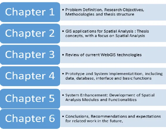
The presented document will be structured in six main chapters.
The present chapter has the objective of determining the project to be executed and document the motivation behind it and the scientific contribution it can represent. Objectives for the project, expectations and intentions are reported within this chapter, along with the resumed structure of the document.
In the second chapter most of the Spatial Analysis related theory to support this project will be presented. Since Spatial Analysis will be the main task performed by the project’s outcome it becomes necessary to explore both the basic concepts as well as some data related topics and spatial analysis methods to be applied during the implementation of the system.
Web-Based GIS will be explored throughout the third chapter with an overview of the existent technology, possible architectures and state of the art. In this chapter other projects’ architecture will be taken into consideration with the objective of defining the most suitable approach towards this subject.
The Prototype and System Implementation will be the theme for the fourth chapter where the most practical part of this project will be explored. The workflow of the project will be presented in the beginning of the chapter and followed through the whole implementation with a more considerate explanation for all the steps from the data collection to the prototype’s implementation. Obstacles and unexpected situations will also be included in this chapter that culminates in the basic implementation of the prototype.
The Project’s outcome will be presented and discussed in the sixth chapter. The achieved result will be explored and analyzed. Modules’ implementation will also be considered in this part of the project as well as the more thorough explanation for each application to be built for this project.
In the last part of this document some conclusions will be drawn regarding this projects’ outcome. Some options for further development within this project’s theme will also be exposed as well as an overview of the technologies used and methods implemented.
7
Figure 2, presented below, summarizes the topics covered in each chapter.
9
2. GIS applications for Spatial Analysis
2.1. Thesis Concepts
2.1.1. Spatial Data
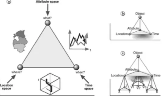
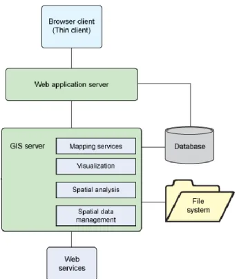
Geographic information concerns objects or phenomena with a specific location in space. Geographical data comprehends geometrical aspects (positions and dimensions), attribute data and temporal data (moment in time in which the data is valid). This logical division is intended to provide an answer to the questions Where? What? And When? Respectively. As can be consulted in figure 3 (Kraak & Ormeling, 2010).
Figure 3 : The characteristics of geospatial data. a. Location, attribute and time, related with the elementary questions Where, What and When, b. the object view, c. detailed characteristics of data components (Source : (Kraak & Ormeling, 2010), p. 4)
Geospatial information has several characteristics that can be further explored in bibliography (Fischer & Getis, 2010; Kraak & Ormeling, 2010; Haining, 2004; Kwakkel et al., 2012), nonetheless, they are summarized in the next paragraph.
Its scale can either be local (as for example analyzing the presence of a species in a specific region) or global (when evaluating sea level rise).
Time is also an important characteristic of geospatial data, since it can either be used to analyze historical data (millions of years to decades), present data (current distribution of an element) or to predict scenarios based on the historical data.
In order to preform data analysis accurately the data must be comparable and compatible. Some of the questions that must be considered when preforming analysis operations comprehend the date when the data was collected, in which way it was
10
collected and for what purpose. These questions make it possible to assure that the utility, reliability and accuracy of the data is compatible with the purpose it was collected for. Different purposes may require different answers to the above referred questions. Data nature defines data according to four different categories: point like objects, linear objects, areal objects and volumetric objects. Measurement units and whether the change is gradual or not (continuous or discrete phenomena’s) will also influence spatial data analysis.
2.1.2. Spatial analysis
‘Spatial Analysis’ is a term that dates back to the 1950s and has a historical evolution that can be consulted in (Berry & Marble, 1968) (p 1- 9).
Even though the most significant advances in geospatial analysis were achieved in with the appearance of GIS, its principles are based on quantitative and statistic geography. Methods of spatial analysis are robust and capable of operating over a range of spatial and temporal scales.
Goodchild & Haining (2004) define it as the ‘collection of techniques and models that explicitly use the spatial referencing associated with each data value or object that is specified within the system under study’, its methods require assumptions about data, describing the spatial relationships or spatial interactions between cases.
Spatial analysis relies on the idea that there is a similarity to nearby attribute values in geographic space, this property was referred by Tobler (1970) as the ‘First Law of Geography’ and is mentioned by (Druck et al., 2004) as spatial dependency.
Cartography, Mathematical modeling and the development and application of statistical techniques are mentioned in the bibliography (Haining, 2004) as the three main elements of spatial analysis, underlining that it is of great importance that the spatial data is adequate to the question to be solved.
2.1.3. Conceptualization and data proprieties
Any process made upon spatial data requires a conceptualization of the real world, in this context it is necessary to identify the proprieties that are relevant to the application (Haining, 2004). It is also necessary to define the adequate presentation to the dataset in question: Level of spatial aggregation and geometric class (point, lines, areas or surfaces).
11
The measurement process is to be considered as the attributes and spatial measurements have to be as precise as possible and defined according to their application. More on scales can be read in the bibliography (Smith et al., 2013).
To resume, “Modeling geographic reality means the process of capturing the complexity of the real world in a finite representation so that digital storage is possible” (Haining, 2004).
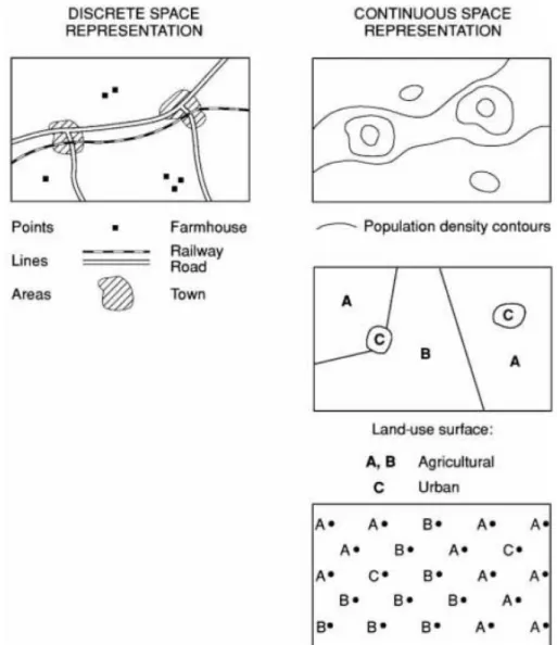
Points, lines, areas and surfaces are the classes of digital objects for representing geographic phenomena, some examples of this are presented in the figure 4 below. Depending on the application of the data it is common to use spatial aggregation to analyze a phenomenon, this leads to a change in the mentioned class.
12
Attribute characteristics can refer to the spatial object themselves or to entities that are associated with or attached to the spatial objects but not directly dependent on them. Conceptualization comes as an essential part of spatial analysis as it refers to the definition and meaning of the attribute. Representation, on the other hand refers to how an attribute is operationalized into variable for the purpose of acquiring and storing data on the attribute and to enable analysis.
Analysis is undertaken on data collected with respect to one or more variables that measure attributes associated with geographic reality that is typically represented into the form of spatial objects. Conceptualization and representation issues of attributes are specific to each particular application.
Haining (2004) presents figure 5 as the schema that defines this process. According to this schema, the real world is represented through to the selected attributes, time and space which constitute the model. Model quality may be assessed in terms of the precision of a representation, its clarity, its completeness, its consistency and resolution. The data matrix (the data structure obtained in order to represent the real world through the mentioned model) will therefore have uncertainty related both to the data model and the data quality.
Buttenfield & Beard (1994) suggest the use of the term accuracy to reflect the correspondence between a representation or conceptualization and what the analyst wishes to measure.
Figure 5 : Conceptualization and Representation, the relationship between the Real World and the Data Matrix. (Source: Haining, 2004)
13 Proprieties of spatial data (Druck et al., 2004):
Spatial dependence is defined by the similarity of values for the same attribute measured at locations near to one another, which is bigger than amongst values separated by larger distance.
If the similarity is constant through the whole area, the dependency structure is defined as stationary, if it varies across the map, it is non-stationary. In the absence of these situations, the structure of dependency is heterogeneous.
The structure of a spatial dependency can display some differences across the axes (north/south, east/west). If the dependency structure is similar along both axes it is called an isotropic dependency structure, if it is not it is called non-isotropic or annon-isotropic.
2.1.4. Data Quality
The definition on data quality is defined by the bibliography as the performance of the data set given the specification of the model, as it depends both on the objective of the appliance of the dataset and the conceptual model to which the data was integrated. According to Salgé (1995), any assessment of data quality from the users’ or producers’ perspective relies on determining how closely data values represent reality given the chosen model for representing that reality.
Even though from an Engineering perspective there’s usually a strong need for precise numbers and accurate approaches to this issue, this approach is far more reasonable when considering to the web environment and to situations where data precision may be far more flexible than for engineering purposes. Regardless the fact that there are several applications in which precision has to be rigorously defined, for this specific project the definition above will suffice, or even be more adequate.
There are several factors to consider when preforming spatial analysis over a dataset, these factors are summarized in table 1 according to the characteristic of data quality concerned and the phase of spatial analysis affected. Even though this topic will not be thoroughly explored within this project, it is of great importance to know the implications and approaches to different degrees of data quality which can be consulted in the literature (Haining, 2004).
14
Table 1 – Dimensions of data quality in relation to stages of spatial analysis. (Source: (Haining, 2004) p. 178 )
2.1.5. Areal Data Problems
Census data and other statistical data are often gathered in areal units for confidentiality purposes or statistical reasons. These areal units are usually delimited by closed polygons inside which it is presupposed to be homogeneous (Druck et al., 2004).
Aggregated data may be used to infer individual-level relationships. The lack of reliable individual-level data is often the cause of using areas to aggregate data.
For the Census case, for example, the target may be of areal level if analyzing the data for administrative sections, regarding the municipality management or the economic factors that are dependent on municipalities’ investment on specific areas. For the Census data case, spatially defined groups may present some degree of homogeneity since as pointed out by Holt et al. (2010), ‘individuals who live in the same area are exposed to common influences and as a result exhibit similarities individuals with similar characteristics choose to live in the same area’. However, aggregation bias is always present, given the rare existence, or inexistence of purely homogenous areal aggregates.
The modifiable areal units problem (MAUP) is explained by Holt et al. (1996, p. 181) as ‘If a statistic is calculated for two different sets of areal units which cover the same population, or sample, a difference will usually be observed even though the same basic
15
data have been used in both analyses. This difference is cited as evidence of the modifiable areal units’ problem’.
For this specific cases, neither the scale of the analysis (choice of number of spatial units) nor their particular configuration (the selected partitioning on zoning given the scale of analysis are fundamental and could, therefor be modified and thus the term ‘modifiable’. The effects of it are addressed by Tobler (1989) and several approaches towards this problem are defined by the bibliography (Haining, 2004, pp.160-173). In this project the aggregation level goes from Civil Parishes to Districts, having three levels of aggregation that can be used according to the user’s object of study. The zoning of the statistical data is aggregated based on administrative boundaries, which are independently managed and have different premises for important areas such as education, family, housing and health.
2.2. Spatial Analysis Methods
Rosenberg (2011), defines four main categories according to the application of the spatial analysis methods. The categories presented bellow will be further explored in the next pages, where special attention will be given to modules to be implemented in the present project.
- Selection : Evolves all the processes from database navigation to display of simple cloropeth maps;
- Manipulation: comprehends all functions that create spatial data, it may be map algebra, geoprocessing, augmenting the capacity of analysis and correlation; - Exploratory analysis: allows the description and visualization of spatial data by
describing patterns of spatial association, suggesting the existence of spatial association, spatial instabilities and identifying atypical observations.
- Confirmatory analysis: includes several models of estimation and validation procedures.
There is a wide range of spatial analysis methods that can be applied to spatial data, depending on the type of data considered. In this particular project, the main data type is areal, as a result of it, the methods presented in this chapter will be limited to those applied for areal data analysis
16 2.2.1. Data Visualization
Graphic display of data aids on detecting data properties. Its visualization can enlighten the viewer (who may or may not be familiar with the data) about specific characteristics of the dataset, being part of a process of understanding and gaining insight into the data. Buja et al. (1960, p.80) define the approaches to data visualization into rendering and manipulation. According to the author, the decision as to what to show in a plot and in particular in deciding what type of plot to construct is what rendering refers to.
Techniques for displaying distributions such as histograms, boxplot, Q-Q and rankit plots and time series (plots) are inserted within univariate data. As for multivariate data, scatterplots, traces and glyphs are mentioned techniques. How to operate on individual plots and how to organize multiple plots in order to explore the data is, according to the mentioned author, what defines manipulation. Tasks included in this approach include finding gestalt (identifying patterns, shapes and other proprieties in the data set), posing queries and making comparisons.
Graphical methods for vizualizing data
Histogram
Histograms are often applied when there are a large number of observations. It consists of a graphical method for displaying the shape of a distribution. A frequency table is used to organize the occurrences o each valued and further along displayed in a bar chart (Lane, 2007).
Box Plot
Box plot or whisker diagram displays the distribution of data based on five characteristics of the dataset: minimum, first quartile, median, third quartile and maximum. The interquartile range (IQR) is represented by the length of the box that is delimited by the first and third quartile. The median is represented by a segment inside the rectangle and the maximum and minimum values by the ‘whiskers’.
A value is considered an outlier if it is 3xIQR above the third quartile or below the first and suspected outlier if it is 1,5xIQR above the third quartile or below the first (Lane 2007).
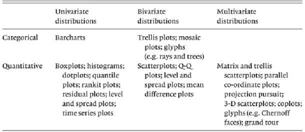
Table 2 resumes the graphical methods used for data visualization.
17
Table 2 – Summary of graphical methods for data visualization. (Source: (Haining,2004), p. 194)
2.2.2. Weights
Weights take a crucial role in several areas of spatial analysis. The spatial matrix expresses, in general terms, the potential for interaction between observations at each pair i,j of locations for a spatial data set composed of n. The structure of these weights can be specified in various ways, and this structure is defined by the spatial weights matrix.
Conceptually, spatial weights define the diagonal ( of a n x n matrix to zero, while the other elements of the matrix reflect the potential of interaction.
There are three main types of weights, according to the elements taken into consideration to the definition of the weight values (Rey, 2013).
1. Contiguity weight matrices reflect the neighbors and weights attributes. There are three different criteria, depending on the definition of neighborhood:
- Rook, which takes as neighbors any pair of cells that share an edge; - Queen, which includes the vertices of the lattice to define contiguities;
- Bishop, which designates pairs of cells as neighbors if they share only a vertex.
2. Distance based weights are generated by taking into consideration the distance between observations. This methods often considers a flat surface which implies that the data should be projected in advanced.
18
- Distance band weights, relies on distance bans or thresholds to define the neighbor set for each spatial unit as those other units falling within a threshold distance of the focal unit;
- Bandwidth determines the distance threshold, the form of the kernel function defines the distance decay in the derived continuous weights.
3. Kernel Weights combines the distance based thresholds together with continuously valued weights.
2.2.3. Exploratory spatial data analysis
Exploratory data analysis (EDA) is defined by She et al. (2012) as a collection of techniques for summarizing data properties (descriptive statistics) and detecting patterns in data, identifying unusual or interesting features in data, detecting data errors, distinguishing accidental from important features in the data set, formulating hypothesis from data .
Furthermore, examining model results, proving whether model assumptions are met and whether there are influential data effects in model fits are also referred as applications of EDA techniques. This set of techniques quantitative summaries of the data that may have a visual representation such as graphs, charts and figures (She et al., 2012).
Spatial Data has its own set of techniques – ESDA, which includes summarizing spatial properties of the data, detecting spatial patterns in data, formulating hypotheses which refer to the geographical distribution of the data, identify cases or subsets of cases that are unusual given their location on the map (Anselin, 2009).The main difference between EDA and ESDA is the spatial component as ESDA extends EDA by adding methods to address special queries that arise as a consequence of the spatial referencing of the data. As a result of it, the map becomes a crucial element in the analysis of the data or examining the model results.
Spatial Autocorrelation
The computational expression of the overall tendency for similar values to be found near together on a map or pertains to the non-random pattern of attribute values over a set of spatial units is called spatial autocorrelation. It can either be positive, meaning that similar values have a tendency to be found together, or negative which reflects a value dissimilarity in space. In both of the referred situations of autocorrelation, the
19
observed pattern is different from what would be expected under a random process operating in space.
There are two different perspective from which autocorrelation can be analyzed (Rey, 2013):
- Global autocorrelation involves the study of the entire map pattern and presents the question of whether the pattern displays clustering or not.
- Local autocorrelation aims to explore within the global pattern to identify clusters or so called hot spots that may be either driving the overall clustered pattern or that reflect heterogeneities that depart from global pattern.
Spatial Autocorrelation indicators are cross product statistics that derive from the expression (Druck et al., 2004):
(1.)
Where is a spatial weight that reflects the spatial relationship between spatial units i and j and is a measurement of correlation between variables.
Global autocorrelation.
Gamma Index of Spatial Autocorrelation.
The principle behind a general cross-product statistic to measuring spatial autocorrelation is applied in the Gamma Index of spatial autocorrelation. In this method, two similarity matrices for n objects are accessed in order to define if they measure the same type of similarity.
Gamma index is defined by the expression (Hubert et al., 1981), consisting of the sum over all cross-products of matching elements (i, j) in the two matrices.
Fundamentally, the first similarity matrix will store a measure of attribute similarity such as cross product, squared difference or absolute difference while the second matrix will be a measure of locational similarity – a spatial weight matrix. Meaning that formally the Gamma Index will be represented by:
20
(2.)
Where represents the elements of the weights matrix and are corresponding measures of attribute similarity.
Moran’s I
The global spatial autocorrelation can be measured using one of the oldest indicators of spatial autocorrelation (Moran, 1948). This indicator is often applied for continuous variables and compares the value of the variable at any location with the value at all other locations. The attribute y measured over n spatial units and is given by Moran’s I as :
(3.)
Where a spatial weight, n is the number of areas that form the study region. where yi is the value that the attribute takes in area i (analogous for the j area) and is the mean value of the attribute in the study region and . Moran’s I can reach values between -1.0 and 1.0, being the amount of autocorrelation defined by the module of the coefficient. It is inexistent when I equals zero and positive or negative according to the index’s signal. (Druck et al., 2004)
Geary’s C
In Geary’s C (Geary, 1954) case the interaction is reflected by the deviations in intensities of each observation location with one another. This indicator is similar to Moran’s I. And is represented by:
(4.) Where a spatial weight, n is is the number of areas that form the study region.
where yi is the value that the attribute takes in area i and is the mean value of the attribute in the study region and .
The index’s result can take values from 0 to 2. Values below 1 indicate negative autocorrelation whereas values equal to 1 indicate no correlation.
21
Getis and Ord’s G
Similarly to the previous statistics, Getis and Ord’s G (1992), is a global measure of spatial association. Representing a multiplicative measure of spatial association of values that fall within a critical distance of each other. However, this index takes values from 0 to 1 and can only be interpreted in comparison with the expected index, which is calculated considering a random distribution.
(5.)
Where d is a threshold distance used to define a spatial weight and yi is the value that the attribute takes in area i (analogous for the j area).
LOCAL Autocorrelation
Local Indicators of Spatial Autocorrelation (LISAs) for Moran’s I and Getis and Ord’s G can be applied to determine clustering.
Local Moran’s I (LISA)
Local Indicators for Spatial Association (Anselin, 1995) are applied to identify local association between and observation and its neighbors up to a specified distance from the said observation. Helps on determining the nature of local distribution.
(6.) Where is a spatial weight, where yi is the value that the attribute takes in area i (analogous for the j area) and is the mean value of the attribute in the study region.
Local G and G*
Getis and Ord can be formalized in two forms: (Ord & Getis, 1995). Comparing local averages to global averages. While Gi* statistic includes the value of the point in its calculation, GI excludes this value, considering the value of its nearest neighbors (within d) against the global average (which also does not include the value of the point itself). It takes values closer to one if there’s a cluster and a small value if there’s a disperse pattern.
22
(7.)
(8.)
Where
Considering that is a spatial weight, n is the number of areas that form the study region, yj is the value that the attribute takes in area j and is the mean value of the attribute in the study region.
Testing indexes’ significance
The Autocorrelation coefficients previously presented need to be tested for statistical significance. This procedure can be performed under two different model assumptions (Smith et al., 2013):
The classical statistical assumption of normality, assuming that the observed value of the coefficient is resultant of a set {zi} of independent and identically distributed values
from a Normal distribution.
In order to perform this tests, the null hypothesis, has to be identified. In this case, for the pattern analysis it is assumed that there is Complete Spatial Randomness (CSR) either of the features themselves or of the values associated with those features.
Z-scores and p-values are therefore calculated to determine whether the null hypothesis must be rejected or not, in this case, rejecting the null hypothesis reveals a statistically significant spatial pattern. The confidence level defines the amount of risk the user is willing to accept for making a false rejection of the null hypothesis (ESRI, 2013). They are summarized in table 3:
23
Table 3 - Normal distibution , z-score, p-value and confidence level (Source:(ESRI, 2013)).
z-score (Standard Deviations) p-value (Probability) Confidence level
< -1.65 or > +1.65 < 0.10 90% < -1.96 or > +1.96 < 0.05 95% < -2.58 or > +2.58 < 0.01 99%
The second model assumes that the observed pattern of the set {zi} of values is
considered just one realization amongst all the possible random permutations of the observed values across all zones. A permutation approach is taken in order to get inference for this statistic, taking the randomization null hypothesis as the basis for statistical significance testing (Smith et al., 2013).
2.2.4. Spatial Regression
Regression analysis allows the process of modeling, examining and exploring spatial relationships facilitating the understanding of the factors that caused observed spatial patterns. These models can be used to predict outcomes based on the used independent variables. A Spatial Regression’s goal is to explain or predict a dependent variable (y), recurring to explanatory variable(s) (x) that is (are) believed to have influence on the dependent variable, as it is illustrated by figure 6.
Such explanation is given by coefficients (β) which values are computed by the regression tool and that reflect both the relationship and strength of each explanatory variable to the dependent variable (Scott, 2009). There is also a part of the dependent variable which is not explained by the model (may be either under or over predicted) which has de name of residuals (ε).
24
In order to define a successful spatial regression model, the variables that have a contribution on the dependent variable have to be thoughtfully chosen.
A (linear) relationship may be of the form (Druck et al., 2004):
(9.)
Where β is a column vector of p parameters to be determined and x is a row of independent variables with a 1 in the first column.
Taking y ={yi} as a set of n observations or measurements of the response variable, with
corresponding recording of matching values for the set of independent variables, then a series of linear equations such as the above can be formulated (Druck et al., 2004). Nevertheless, since the number of observations is usually greater than the number of coefficients, the best fit solution can be a possible approach to this situation. The best fit in this case will be the solution for vector β that minimizes the difference between the fitted model and observed values at these data points.
Ordinary Least Squares (OLS)
Least squares is the term applied to the procedure of minimizing the sum of the squared differences and is often applied. In this case ε is a vector of errors that in conceptual terms is assumed to represent the effects of unobserved variables and measurement errors in the observations. The expected value of this error E(ε)=0 and the variance E(εε)=σ2 I is constant. Where I is the identity matrix.
In this context, the set of n equations is typically solved for the vector β that minimizes the sum of the squares error terms, εεT, hence the name Ordinary Least Squares or OLS (Smith et al., 2013).
The solution for the coefficients using this approach is obtained from the matrix expression(Smith et al., 2013):
(10.)
And (11.)
The variance for such models is usually estimated from the residuals of the fitted model using the expression:
25
In the spatial context, the objective is to model the variation in some spatially distributed dependent variable, from a set of independent variables. Conceptually, the form of the chosen model should be as simple as possible, both in terms of the expression employed and the number of independent variables included. Moreover, the correlation between different independent variables should be as low as possible and the proportion of the variation in the dependent variable(s), y, explained by the independent variable (X) should be as high as possible. When there is a high correlation among some or all the independent variables (x), (usually reflected by a correlation coefficient above 0.8) the model is almost certain to have redundant information and may be described as being over-specific (Haining, 2004).
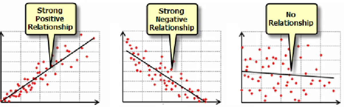
The coefficient signal (+/-) of each explanatory variable indicates if the relationship is either positive or negative, as illustrated by figure 7.
Figure 7 : Illustration of spatial relationship according to the explanatory variables signal. (Source: (Scott, 2009))
Multi-colinearity is said to exist if the there is a strong relationship between selected independent variables and is also broadly linear. To reduce multi-colinearity there are several techniques, such as: applying a so-called centering transform (by deducting the mean of the relevant independent variable from each measured values), increasing the sample size (used specially for small samples); removing the most inter-correlated variable or combining inter-correlated variables into a new single composite variable. Heteroskedasticity is said to exist if the spread of errors is not constant. When fitting a model using OLS it is generally assumed that the errors (residuals for sample points) are identical and independently distributed.
In this case the estimated variance under OLS will be biased, resulting in non-reliable specification for confidence intervals and standard statistical significance tests (e.g. F tests)
26
Model performance can be assessed using several statistics mentioned in standard statistical bibliography (Scott, 2009).
Spatial autoregressive modeling
Pure spatial autoregressive model consists of a spatially lagged version of the dependent variable,y (Druck et al., 2004):
(13.)
Despite its similarity to a standard linear regression model, the first term is constructed by a predefined n by n spatial weighting matrix, W, applied to the observed variable y. together with a spatial auto regression parameter, p, which typically has to be estimated. According to Anselin (2008, p257), spatial lag models are ‘a formal representation of the equilibrium outcome of processes of social and spatial interaction’.
A spatial lag model can reflect some kind of interaction effect by expressing the notion that the value of a variable at a given location is related to the values of the same variable measured at nearby locations.
Adjusted R2 (a modification of the statistic mentioned above), considers the complexity of the model in terms of the number of variables that are specified.
The dynamics of longitudinal spatial data or observations on fixed areal units over multiple time periods can be analyzed by several exploratory approaches.
Statistical Significance
Squared coefficient of (multiple) Correlation or coefficient of determination (R2). This statistic records the proportion of variation in the data that is explained by the models, as it is the function of the squared residuals with standardization being achieved using the sum of squared deviations of observations from the overall means:
(14.)
Where εi represents the residual for the observation, yi is the value for that specific
observation and is the mean value for the observations.
If determined under appropriate conditions, this coefficient will take values close to 1 if highly significant. However, it is frequent not to be able to determine the statistical