REM WORKING PAPER SERIES
Sovereign Indebtedness and Financial and Fiscal Conditions
António Afonso, João Tovar Jalles
REM Working Paper 0111-2019
December 2019
REM – Research in Economics and Mathematics
Rua Miguel Lúpi 20, 1249-078 Lisboa,
Portugal
ISSN 2184-108X
Any opinions expressed are those of the authors and not those of REM. Short, up to two paragraphs can be cited provided that full credit is given to the authors.
1
Sovereign Indebtedness and Financial and
Fiscal Conditions
*
António Afonso
$João Tovar Jalles
#November 2019
Abstract
We empirically assess the magnitudes of sovereign indebtedness responses for a sample of 123 Advanced and Emerging Market Economies, between 1980 and 2018, taking into account the changing characteristics of financial markets, notably the Global and Financial Crisis. Our results show that when the financial conditions are more stressful, for instance, higher yield spreads or a heightened degree of financial stress, fiscal authorities use more actively their primary balance to reduce sovereign indebtedness, which is not the case when financial market conditions are more benign. This is notably true for the case of Emerging Market Economies sovereigns, who most likely then struggle more to fund themselves.
JEL: C23, G15, H63
Keywords: sovereing indebtdness, panel data, financial stress, global financial crisis, emerging markets
_____________________________
* The opinions expressed herein are those of the authors and do not necessarily those of their employers. Thanks
go to the editor and two anonymous referees for useful comments and suggestions.
$ ISEG-UL – Universidade de Lisboa; REM – Research in Economics and Mathematics, UECE – Research Unit
on Complexity and Economics. R. Miguel Lupi 20, 1249-078 Lisbon, Portugal. UECE is supported by FCT (Fundação para a Ciência e a Tecnologia, Portugal), email: aafonso@iseg.utl.pt.
# UECE – Research Unit on Complexity and Economics and REM – Research in Economics and Mathematics.
R. Miguel Lupi 20, 1249-078 Lisbon, Portugal. UECE is supported by FCT (Fundação para a Ciência e a Tecnologia, Portugal). Centre for Globalization and Governance and Economics for Policy, Nova School of Business and Economics, Rua da Holanda 1, 2775 Carcavelos, Portugal. email: joaojalles@gmail.com.
2
1. Introduction
After the recent Global Financial Crisis (GFC) and in the context of important restrictions to the implementation of fiscal policies, notably in Advanced Economies (AE) and in some Emerging Market Economies (EME), the appraisal of how fiscal authorities adjust to financial developments is quite important.1 For instance, it is useful to assess whether the track record as been one of more active (less Ricardian) or more passive fiscal developments in several groups of homogenous economies, which can hint at the future expected reaction from the fiscal authorities.
Moreover, it is true that the level of government indebtedness increased to record levels in the context of the GFC, linked (in a vicious cycle) notably to heightened financial stress in capital markets and to higher sovereign yield spreads demanded by potential investors due to uncertainty reasons. At the same time, the ensuing downgrading of sovereign ratings contributed to the increase in the difficulties of sovereigns’ access to capital markets. Global debt reached the record peak of US$164 trillion in 2016, equivalent to 225 percent of global GDP (IMF, 2018). The world is now 12 percent of GDP deeper in debt than the previous peak in 2009.
The existing literature has estimated fiscal policy response functions notably in a cross-country analysis setup. In this context, based on the economic rationale that governments care about fiscal sustainability issues, it is possible to envisage a simple fiscal reaction function in which the primary balance improves to counteract past increases in government debt (Bohn, 2008; Ballabriga and Martinez-Mongay, 2005; and Afonso, 2008). In addition, the existence of possible cross-section dependencies, notably given the economic and financial interlinkages in advanced (emerging market) economies, capital markets integration, common monetary policy for the euro area countries, has been scarcely addressed within this framework.
Against this background, we empirically assess the magnitudes of sovereign indebtedness responses for sovereign indebtedness for a sample of 123 AE and EME, between 1980 and 2018, taking into account the changing characteristics of the financial markets, notably the GFC. This analysis is then in the vein of the FTPL discussion, where fiscal policy may have a relevant role, at least as important as monetary policy, in determining the price level. 2
_____________________________
1 Some researchers have examined financial sector and crisis-related determinants of sovereign bond spreads (se
e.g. Ebner (2009) and Dailami, Masson, and Padou (2008)).
3
2. Empirical Methodology
We set up a sovereign debt reaction function (see Canzoneri et al., 2001; Afonso, 2008; and Bohn, 2008) to assess whether the primary budget balance negatively affects government liabilities. We can estimate the following relationship for country i and time t:
∆Bit= ∆γ sit−1+ ∆ϕ Bit−1+ ∆β zit+ ∆uit. (1)
Equation (1) is compatible with the standard budget deficit and debt dynamics formulation, where government debt (B) changes due notably to the primary balance (s). When γ <0, most likely the government uses budget surpluses to reduce outstanding government debt. In addition, the output gap (z) – the difference between the actual output and potential output (expressed as percentage of potential) – controls for the reaction of debt to the business cycle. uit is a standard white noise disturbance. The option of using first differences is to avoid
potential stationarity issues, an approach followed for instance by Afonso (2008) and Canzoneri et al. (2001).
We begin by estimating (1) with a pooled OLS estimator (augmented with country and time effects included to control, respectively, for all time-invariant differences across countries – such as geographical characteristics - and for global shocks - such as shifts in oil prices or the global business cycle). The first-differenced equation should take care of stationarity issues, however it introduces a correlation between the differenced lagged dependent variable and the differenced error term, hence, the use of instruments is required. Consistent estimates can be obtained employing a two-stage least squares (TSLS) estimator and relying on instrumental variables (IV) which are correlated with ∆sit−1(∆Bit−1) and
orthogonal to∆vit(∆uit). Indeed, lagged values ∆sit−2and Bit−2satisfy these assumptions and can be used as IV for the first-differenced equation (1). To address potential endogeneity concerns, we also rely on a system GMM estimator (Arellano and Bover, 1995). For robustness purposes, other (more recent) estimators that are arguably preferable since they explicitly deal with cross-sectional dependencies, are also employed. First, we re-run (1) with a panel estimation allowing for Driscoll-Kraay (1998) robust standard errors. Then, we use the Mean Group (MG) estimator (Pesaran and Smith, 1995). In addition, we rely on the Common Correlated Effects Pooled estimator that accounts for the presence of unobserved common factors. In its heterogeneous version, the Common Correlated Effects Mean Group (CCEMG), the presence of unobserved common factors is achieved by construction and the
4
estimates are obtained as averages of the individual estimates (Pesaran, 2006). Yet another recent approach is due to Eberhardt and Teal (2010), termed Augmented Mean Group (AMG) estimator, and it accounts for cross-sectional dependence by including of a “common dynamic process”.
As far as data is concerned, we use annual data for 123 countries over 39 years that is, focusing on the period 1980-2018. The fiscal data comes from the IMF’s Government Finance Statistics database. In addition, we use the output gap to control for business cycle fluctuations. The fiscal data comes from the IMF’s Government Finance Statistics database. Despite substantial progress in the estimation methodologies to calculate potential output, there is still not a widely accepted approach in the profession. Researchers adopt two alternative approaches to estimate potential GDP (Borio, 2013): i) there are univariate statistical approaches, which usually consist of filtering out the trend component from the cyclical one; ii) there are the structural approaches, which derive the estimates directly from the theoretical structure of a model. In the present paper, we opt for the first approach, that is, the output gap is computed using the Hodrick-Prescott filter (as standard practice in the literature).3
As far as panel stationarity is concerned, results of first (Im-Pesaran-Shin, 1997) and second-generation (Pesaran, 2007) panel integration tests are available upon request for reasons of parsimony. Essentially, we can accept most conservatively that non-stationarity cannot be ruled out in the main variables of interest in levels.
3. Empirical Analysis
In Table 1 we report our baseline results. It is possible to see that, indeed, better fiscal positions (higher primary balances) translate into lower sovereign debt ratios. In addition, such reaction is statistically less significant after the GFC. This can be interpreted as a bigger part of the increase in sovereign debt being at that time probably more related to the so-called stock-flow adjustments. These in many cases stemmed from the materialization of contingent liabilities that countries had to absorb in their public accounts. In addition, it seems that the
_____________________________
3 Alternatively we also employed the IMF’s WEO output gap which yielded qualitatively similar results, even at
the cost of a smaller number of observations. In fact, the bivariate correlation between the common set of WEO and HP-generated output gaps was 85 percent in our sample. The reason why the WEO output gap was not used as the baseline relates to the fact that these estimates are problematic in a cross-country analysis as they are based on methodologies that vary by country desk. As such, differences in gap estimates across countries are also due to the different methodologies used, rather than differences in economic fundamentals.In addition, by applying a filter we maximize the total number of observations available in a consistent and uniform manner.
5
coefficient of changes of primary balances is larger (in absolute value) in the subsample of AEs relative to EMEs.
[Table 1]
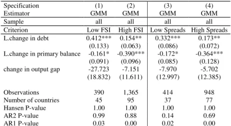
In Table 2 we account for financial conditions present in the markets and rely on the system GMM estimator (results using other estimators available upon request). Note that due to data availability constraints Tables 2 and 3 are estimated with data until 2014.4 In other words, we split the sample considering the cases above and below the subsample median (that is, either the subsample of AE or EME) of the Financial Stress Indicator (FSI) and of sovereign bond spreads vis-à-vis the USA.5 It is important to notice that when financial conditions are more stressful, governments more actively use primary balances to curb down sovereign indebtedness. This is notably true in the EMEs sub-sample, which is not the case when financial market conditions are more benign, where almost no statistically significant effect can be uncovered between the primary balance and the debt ratio. In the case of AEs, the Ricardian behaviour is present in both cases.
[Table 2] [Table 3]
Moreover, the magnitude the response of debt to higher primary balances, in dire financial conditions, is also higher and more statistically significant in the cases of high spreads, for the EME and AE subsamples, which may imply that sovereigns struggle more to finance themselves in capital markets in those periods. Spreads are a measure of a country’s overall risk premium, stemming from market, credit, liquidity, and other risks. EMEs during times of hardship are typically characterized by a higher degree of uncertainty (relative to AEs) leading to higher prices demanded on their sovereigns. This finding is consistent with the view that crisis periods adversely affect the ability of sovereign issuers to service their debt,
_____________________________ 4
The FSI data are only available until 2014. We use the spreads data ending also in 2014 for comparability purposes.
5 The FSI variable was retrieved from Balakrishnan et al. (2009) extended to 2014. This index represents an
important improvement vis-à-vis zero-one binary variables, as it measures the intensity of stress and it is not ambiguous regarding ‘near-miss’ events. Moreover, it covers both abrupt rises in risk and uncertainty, concerns about the health of the financial sector, large swings in asset prices and sudden drops in liquidity.Bond yields come from Datastream and Bloomberg and the spread was computed vis-à-vis the US benchmark.
6
which is reflected in the premium on their bond yields.6 This conclusion is also valid for the case when the full country sample is used instead (see Table 3).
Finally, we re-estimated the baseline analysis using alternative estimators as a robustness check. In addition, we also split the sample by geographical regions (Europe, Western Hemisphere, Africa, and Asia and Middle East) and the time span by decade.
Table 4 summarises the signs (positive or negative) of the obtained estimated coefficients of the change in primary balances (and also whether the obtained coefficients were statistically significant). We get the confirmation of the estimated negative coefficient for the cases of Europe and Western Hemisphere., while there is no statistically supported reaction in the case of the African, and Asian and Middle Eastern country sub-samples. Moreover, we can observe that, while in the sub-period 2000-2010 there is a statistically significant effect of the primary balance in reducing sovereign indebtedness, that effect is no longer significant in the period of the crisis (2010-2014), confirming our baseline results (recall Table 1).
[Table 4]
4. Conclusions
We assessed the magnitudes of sovereign indebtedness responses for sovereign indebtedness for a sample of AE and EME, between 1980 and 2018.
We found that when the financial conditions are more stressful, for instance, higher yield spreads or higher financial stress, fiscal authorities use more actively the primary balance to reduce sovereign indebtedness, which is not the case when financial market conditions are more benign. This is notably true for the case of EMEs.
Policy implications are twofold: i) adverse financial conditions put more pressure onto fiscal authorities that make an effort to keep their debts on track more actively; that is, stringent financial conditions act as a disciplinary mechanism; ii) after the 2008-10 GFC it seems plausible that other (key) factors, over and beyond that coming from budgetary imbalances, end up showing up in the stock of sovereign debt.
_____________________________
6 Bellas et al. (2010) findings indicate that financial sector vulnerabilities appear to be a crucial factor in
7
References
1. Afonso, A. (2008), “Ricardian Fiscal Regimes in the European Union”,
Empirica, 35 (3), 313–334.
2. Arellano, M., Bover, O. (1995), "Another Look at the Instrumental Variable Estimation of Error Component Models", Journal of Econometrics, 68: 29-51. 3. Balakrishnan, R., S. Danninger, S. Elekdag, and I. Tytell. 2009. The Transmission
of Financial Stress from Advanced to Emerging Economies. IMF Working Paper WP/09/133. Washington, DC: International Monetary Fund (IMF).
4. Ballabriga, F., Martinez-Mongay, C. (2005). “Sustainability of EU public finances,” European Commission, Economic Papers No 225, April.
5. Bellas, D., Papaionannou, M., Petrova, I. (2010), “Determinants of emerging markets sovereign bond spreads: fundamentals vs financial stress”, IMF WP series No. 10/281.
6. Bohn, H. (2008). “The Sustainability of Fiscal Policy in the United States,” in Neck, R., Sturm, J.-E. (eds.), Sustainability of Public Debt. The MIT Press, Cambridge, Massachussets.
7. Borio C., Disyatat P., Juselius M. (2013), Rethinking Potential Output: Embedding Information about the Financial Cycle, BIS Working Papers, n.404.Canzoneri, M., Cumby, R., Diba, B. (2001). “Is the Price Level Determined by the Needs of Fiscal Solvency?” American Economic Review, 91(5), 1221-1238.
8. Canzoneri, M., Cumby, R., Diba, B. (2001). “Is the Price Level Determined by the Needs of Fiscal Solvency?” American Economic Review, 91(5), 1221-1238. 9. Dailami, M., Masson, P., Padou, J. (2008), “Global Monetary Conditions versus
Country-Specific Factors in the Determination of Emerging Market Debt Spreads,” Journal of International Money and Finance, 27(8), 1325–36. 10. Driscoll, J., Kraay, A. (1998), "Consistent Covariance Matrix Estimation with
Spatially Dependent Panel Data", Review of Economics and Statistics, 80(4), 549-560
11. Eberhard, M., Teal, F. (2011), “Econometrics for Grunblers: A new look at the literature on cross-country growth empirics”, Journal of Economic Surveys, 25(1), 109-155.
12. Ebner, A. (2009), “An Empirical Analysis on the Determinants of CEE Government Bond Spreads,” Emerging Markets Review, 10, 97–121.
13. Evans, P. (1997), “How fast do economies converge”, Review of Economics and
Statistics, 79(2), 219-25.
14. Im K.S., Pesaran M.H., Shin, Y. (1997) Testing for Unit Roots in Heterogeneous Panels, mimeo Cambridge University Lee, K., M.H. Pesaran and R. Smith (1997), “Growth and convergence in a multi-country empirical stochastic Solow model”,
Journal of Applied Econometrics, 12, 357-392.
15. IMF (2018), “Capitalizing on Good Times”, IMF Fiscal Monitor, April 2018, Washington DC.
16. Leeper, E. (1991). “Equilibria Under 'Active' and 'Passive' Monetary and Fiscal Policies,” Journal of Monetary Economics, 27 (1), 129-147.
17. Pesaran, M. H. (2006), “Estimation and inference in large heterogeneous panels with a multifactor error structure”, Econometrica, 74(4), 967-1012.
18. Pesaran, M. H. (2007), “A simple panel unit root test in the presence of cross-section dependence”, Journal of Applied Econometrics, 22, 265-312.
19. Pesaran, M.H., Smith, R. (1995), “The role of theory in econometrics”, Journal
8
Table 1. Baseline Results (1980-2018)
(1) (2) (3) (4) (5) (6) (7)
Estimator OLS IV GMM GMM GMM GMM GMM
Sample all all all AE EME all all
Time Spain all all all all all Before GFC After GFC L.change in debt 0.204*** 0.217*** 0.223*** 0.386*** 0.193** 0.219*** 0.238***
(0.035) (0.041) (0.066) (0.088) (0.074) (0.070) (0.089) L.change in primary balance -0.091*** -0.094*** -0.027* -0.253** -0.028* -0.023** -0.107
(0.019) (0.020) (0.015) (0.113) (0.015) (0.009) (0.118) change in output gap -0.003* -0.004 -0.004** -0.179 -0.004* -0.003** -0.022
(0.002) (0.003) (0.002) (0.188) (0.002) (0.001) (0.021) Observations 2,799 2,675 2,799 943 1,853 1,851 1,894 Number of countries 123 123 123 36 87 123 123 R-squared 0.273 0.111 Hansen P-value 0.56 0.71 0.87 0.42 0.72 AR2 P-value 0.126 0.203 0.182 0.118 0.261 AR1 P-value 0.012 0.002 0.003 0.001 0.008 Note: “GFC” denotes Global Financial Crisis (corresponding to 2007/08). “L” denotes the lagged variable. Robust standard errors in parenthesis clustered at the country level. The Hansen test evaluates the validity of the instrument set, i.e., tests for over-identifying restrictions. AR(1) and AR(2) are the Arellano–Bond autocorrelation tests of first and second order (the null is no autocorrelation), respectively. Time and country fixed effects were included, but are not reported. Also, a constant term has been estimated but it is not reported for reasons of parsimony. *, **, *** denote statistical significant at the 10, 5 and 1 percent level, respectively.
Table 2. Accounting for financial conditions, AE vs EME (1980-2014)
(1) (2) (3) (4) (5) (6) (7) (8)
Estimator GMM GMM GMM GMM GMM GMM GMM GMM
Sample AE AE AE AE EME EME EME EME
Criterion Low FSI High FSI Low Spreads High Spreads Low FSI High FSI Low Spreads High Spreads L.change in debt 0.361** 0.272*** 0.390*** 0.371*** 0.331** 0.174 -0.021 0.170
(0.167) (0.077) (0.098) (0.132) (0.119) (0.127) (0.127) (0.131) L.change in primary balance -0.222** -0.283** -0.134 -0.241*** -0.241 -0.441*** -0.464 -0.412***
(0.083) (0.105) (0.101) (0.082) (0.478) (0.149) (0.425) (0.122) change in output gap -44.210* -12.582 -12.933 -6.693 -10.032 -1.474 -18.782 -1.151 (21.565) (12.374) (16.899) (18.121) (55.276) (15.907) (38.457) (15.816) Observations 287 529 397 419 136 632 130 638 Number of countries 25 35 33 30 20 48 17 46 Hansen P-value 1.00 1.00 1.00 1.00 1.00 1.00 1.00 1.00 AR2 P-value 0.76 0.99 0.13 0.25 0.76 0.18 0.11 0.60 AR1 P-value 0.09 0.01 0.02 0.01 0.02 0.07 0.06 0.03
Note: “L” denotes the lagged variable. Robust standard errors in parenthesis clustered at the country level. The Hansen test evaluates the validity of the instrument set, i.e., tests for over-identifying restrictions. AR(1) and AR(2) are the Arellano–Bond autocorrelation tests of first and second order (the null is no autocorrelation), respectively. Time and country fixed effects were included, but are not reported. Also, a constant term has been estimated but it is not reported for reasons of parsimony. *, **, *** denote statistical significant at the 10, 5 and 1 percent level, respectively.
9
Table 3. Accounting for financial conditions, whole sample (1980-2014)
Specification (1) (2) (3) (4)
Estimator GMM GMM GMM GMM
Sample all all all all
Criterion Low FSI High FSI Low Spreads High Spreads L.change in debt 0.412*** 0.154** 0.332*** 0.173**
(0.133) (0.063) (0.086) (0.072) L.change in primary balance -0.161* -0.390*** -0.172* -0.364***
(0.091) (0.096) (0.085) (0.128) change in output gap -27.723 -7.151 -7.970 -5.702
(18.832) (11.611) (12.997) (12.385) Observations 390 1,365 414 948 Number of countries 45 95 37 77 Hansen P-value 1.00 1.00 1.00 1.00 AR2 P-value 0.99 0.88 0.14 0.69 AR1 P-value 0.03 0.00 0.02 0.00
Note: “L” denotes the lagged variable. Robust standard errors in parenthesis clustered at the country level. The Hansen test evaluates the validity of the instrument set, i.e., tests for over-identifying restrictions. AR(1) and AR(2) are the Arellano–Bond autocorrelation tests of first and second order (the null is no autocorrelation), respectively. Time and country fixed effects were included, but are not reported. Also, a constant term has been estimated but it is not reported for reasons of parsimony. *, **, *** denote statistical significant at the 10, 5 and 1 percent level, respectively.
Table 4. Robustness Checks and Sensitivity (1980-2018) Effect of change in debt on…
Robustness Estimators
Driscoll-Kraay
CCEMG MG AMG
L.change in primary balance (controlling for change
in output gap)
-0.096*** -0.276*** -0.193*** -0.287***
Geographical Regions (with GMM) Europe Western
Hemisphere
Africa Asia and Middle East L.change in primary balance (controlling for change
in output gap)
-0.323*** -0.280* -0.034 -0.118
Time split (with GMM) 1980-1990 1990-2000
2000-2010
2010-2018 L.change in primary balance (controlling for change
in output gap)
-0.256** -0.017** -0.185** -0.140 Note: Estimation of (1). “L” denotes the lagged variable. For further details on the estimators refer to the main text. *, **, *** denote statistical significant at the 10, 5 and 1 percent level, respectively.