Estimation of the Agricultural Probability of Loss:
evidence for soybean in Paraná State
Vitor Augusto Ozaki1, Ricardo Olinda2,
Priscila Neves Faria3 and Rogério Costa Campos4
Abstract: In any agricultural insurance program, the accurate quantification of the probability of the loss has great importance. In order to estimate this quantity, it is necessary to assume some parametric probability distribution. The objective of this work is to estimate the probability of loss using the theory of the extreme values modeling the left tail of the distribution. After that, the estimated values will be compared to the values estimated under the normality assumption. Finally, we discuss the implications of assuming a symmetrical distribution instead of a more flexible family of distributions when estimating the probability of loss and pricing the insurance contracts. Results show that, for the selected regions, the probability distributions present a relative degree of skewness. As a consequence, the probability of loss is quite different from those estimated supposing the Normal distribution, commonly used by Brazilian insurers.
Key-words: Risk, extreme value theory, probability of loss, crop insurance.
Resumo: Em todo programa de seguro agrícola, a quantificação da probabilidade da perda da produtividade agrícola é de grande importância. A fim de estimar esta quantidade, é necessário supor alguma distribuição de probabilidade paramétrica. O objetivo deste trabalho é estimar a probabilidade da perda usando a teoria dos valores extremos para modelar a cauda esquerda da distribuição. Os valores estimados foram comparados aos valores estimados sob a suposição da normalidade. Por fim, são discutidas as implicações de se supor uma distribuição simétrica em vez de uma família mais flexível de distribuições para estimar a probabilidade da perda e fixar a taxa de prêmio dos contratos de seguro. Os resultados mostraram que, diferente dos procedimentos adotados no mercado segurador, que supõem normalidade, as distribuições de probabilidade apresentam um relativo grau de assimetria que modifica o valor das probabilidades de perda e, consequentemente, as taxas de prêmio.
Palavras-chave: Teoria dos valores extremos, risco, probabilidade de perda, seguro agrícola.
JEL Classification: C00.
1. Professor no Departamento de Economia, Administração e Sociologia da ESALQ/USP e coordena-dor do GESER/ESALQ. E-mail: [email protected]
Historically, Brazilian agricultural insurance market faces some well recognized problems. More specifically, insurance high costs, systemic nature of risk, adverse selection, lack of accurate farm-level information, and moral risk can be pointed out as the main drawbacks.
Recently, the Federal Government has implemented some initiatives to develop crop insurance in Brazil. For instance, by the Federal Law 10,823 part of the total insurance costs will be subsidized. Now, the following step relies on providing information to drive rules by which the insurance companies will offer their products. It implies in getting around the problem concerning the lack and inaccurateness of the information exhibited in some areas.
Remarkably, the insurance market is based on individual information which is important to show the risk profile of each one. In the absence of reliable and accurate information insurers will avoid offer their contracts. In the agricultural sector farm-level yield data is almost inexistent. Some cooperatives have gathered yield information from their associated producers, but it is still far from being enough to support the spatial density of information which is demanded by the crop insurance. Municipality-level yield has been recorded and released by
aggregation is not desirable for local (farming fields) risk analysis (OZAKI, 2008).
According to the IBGE the Parana State is the major grain producer in Brazil. In 2011, the IBGE estimated a high production of soybean (13.4 millions of tons). This amount is 41% larger, when compared to the total reached in the previous harvest year. However, less than 10% of the planted area is covered by crop insurance. In this context, the analyses of the probability of loss can support insurance companies to deal with seasonal fluctuation of grain production. Traditionally, the Normal distribution assumption is commonly used by the insurers to quantify and price the risk. Nevertheless, by assuming the Normal distribution it is not possible to take into account the skewness and bimodalities present in the probability distributions of the agricultural yields (GOODWIN and KER, 1998).
heavier tails as in extreme values distributions (OZAKI et al., 2008).
In the literature, Just and Weninger (1999) suggest the normality assumption, whilst others point out evidences against it (DAY, 1965; TAYLOR, 1990; RAMIREZ et al., 2003). Alternatively, Beta distribution (NELSON and PRECKEL, 1989; TIRUPATTUR, HAUSER and CHAHERLI, 1996; BABCOCK, HART and HAYES, 2004; and COBLE et al., 1997), Inverse Hyperbolic Sine Transformations (MOSS and SHONKWILER, 1993; RAMIREZ, 1997), Log-Normal (GOODWIN, ROBERTS and COBLE, 2000), Skew Normal distributions (OZAKI and SILVA, 2009) and Gamma (GALLAGHER, 1987) have been proposed.
This study applies the extreme value theory to model the left tail of the agricultural yield probability distribution of the mesoregions5 in Parana state. Finally, the estimates are compared to those supposing the Normal distribution that is commonly used by insurance companies.
The paper is organized as follows: in Section 2 we briefly review some aspects of crop insurance. In Section 3 we show the extreme value theory and in Section 4 we describe the Brazilian yield data for soybean. In Section 5 we present our empirical findings and discuss their implications, and in Section 6 we conclude the paper.
2. Crop insurance
Basically, the compensation mechanism is triggered by the farm-level yield. Producers are indemnified when the agricultural yield observed in the end of the harvest (in the unit or farm) falls below the yield guaranteed in the contract. This type of agricultural insurance is called individual yield crop insurance. The indemnity I for each farm i can be expressed as follows:
, max
Ii i xi x 0
c i
φ
= 6^ − h @
5. Groups of municipalities within a State with common
cha-In which:
φi is the deductibility, 0 < φi < 1;
xi c
is the critical yield;
xi is the observed (final) yield;
The critical yield is defined according to the equation: xc = αiμi. In which: αi is the level of
coverage chosen by the agricultural producer, 0 < αi < 1; and, μi is the farmer expected yield. In
what follows, Ii represents the indemnity due to
each producer when the agricultural yield xi falls
below the guaranteed yield xi c
.
3. Methodology
Extreme value theory (EVT) is widely applied in financial, economical and insurance areas. One of the main challenges to the risk manager is to implement risk management models which allow for rare and damaging events with perverse consequences (KOEDIJK et al., 1990; LORETAN and PHILLIPS, 1994; LONGIN, 1996; EMBRECHTS et al., 1997; DANIELSSON and DE VRIES, 2000; NEFTCI, 2000; MCNEIL and FREY, 2000; GENCAY et al., 2003; DIEBOLD et al., 1998).
The regulator agents of insurance companies expect the companies be able to honor their contracts even under crises scenarios. Thus, it is mandatory to keep a reasonable fund to avoid insolvency in case of catastrophic events.
EVT has become one of the main theories in developing statistical models for extreme insurance losses. This approach is focused on a special class of probability distributions called Generalized Extreme Value distribution (GEV) which encompass distributions like Gumbel, Fréchet and Weibull. PGD (Pareto Generalized Distribution) distribution such as Exponential, Pareto and Beta are also used in the EVT approach as well. In the standard format GEV and PGD depend only on the parameter which is called tail index.
values over some threshold; and, the Block Maxima (or Gumbel method) approach addresses the set of maximum values coming from a block of observations. In order to assess the market risk, for instance, the Block Maxima is used to estimate the return probability of maximum (minimum) event for a given time interval (e.g., months, years) (DE HAAN and PEREIRA, 2006).
3.1. Extreme value theory
Suppose that the sequence X1, X2, ... Xn is independent and identically distributed (i.i.d.) with distribution function F(X) and let ϒn =
max(X1, X2, ... Xn) with distribution function: Pr{ϒn≤x} = Pr{X1 ≤x, ..., Xn≤x} = (F(x))n
Then ϒn has the distribution function
. ..
. ..
limPR a x b limPR
a b
x Hx
n n n n n n
n n
# + = − # =
"3 "3
^ h =^ h G (1.1)
In which an > 0 and bn are normalized
constants.
If (1.1) holds, we say F (or X) belongs to the (maximum) domain of attraction (MDA) of H and write F ∈ MDA(H) (or X ∈ MDA(H)). Note that H has one of the following three parametric forms (which are generally called Extreme Value Distributions - EVD):
: , : , , : , , exp exp exp exp
Type I H x x all x
Type II H x
x if x if x
Type III H x x if x if x 0 0 0 1 0 0 2 1 # $ = − − = − = − a a -^ ^ ^ ^ ^ ^ ^ h h h h
h h h
"
)
)
,
(1.2)
In II and III α is any positive number. The three types are also often called the Gumbel, Fréchet and Weibull distributions, respectively.
3.1.1. Fisher-Tippett Theorem
Let ϒn = max(X1, X2, ..., Xn) be a sequence of
independent and identically-distributed random variables. For some an > 0 let:
ϒ ϒ
.
Pr"an-1^ n−bnh#x,"H x^ h (1.3)
for some non-degenerate H then it belongs to the three types described in 1.2.
Based on the Fisher-Tippett theorem is possible to estimate the asymptotic distribution of
.
a b
n n− n
^ h
directly from the family H without the
distribution of X. The three types of extreme value distributions can be written into a generalized extreme value (GEV) distribution form given by
; , , exp
H x 1 x
/
1
µ σ ξ
σ
ξ µ
= − + −
p
-^ h ) = ^ hG 3
in which µ, σ and ξ are the parameters of location, scale and shape, respectively. Moreover, 1 +
ξ(x – µ)/σ > 0, σ > 0. The case where ξ = 0 is interpreted as the limit case ξ→ 0, that is
; , , exp exp
H xµ σ0 x
σ µ
= − − −
^ h ) = ^ hG3
Type II and III correspond to ξ20 ξ 1 α =
c m
and ξ10 ξ 1
α = −
c m respectively6.
The Fisher-Tippett theorem gives a limit distribution for the maximum collected in a block of size n. Let x1,x2,...,xk be observations of the
random variable X. The sample data is partitioned into n blocks such that nk≤m, and let
ϒ1 = max{x1,...,xk} ϒ2 = max{xk-1,...,x2k} ..
.
ϒn = max{xnk-k+1,...,xnk}
The estimators of µ^, σ^ and ^ξ
are estimated using this new sample, ϒ1,ϒ2,...,ϒn.
From the GEV we can get the probability density function of the GEV distribution given by:
; , , exp
f xX 1 1 x 1 x
1 1
µ σ ξ
σ ξ σ
µ
ξ σ
µ
= + − p − + −
p
p
- +
-^ c c
f
h m m
p
; E ) ; E 3
6. Smith (1990) detailed the statistical treatments, applica-tions and estimaapplica-tions of the GEV.
ϒ
in which -∞ < x < (µ - σ)/ξ for ξ < 0, and (µ - σ)/ξ < x < +∞ for ξ > 0 in which x is a random variable associated to the maximum values. Suppose now that Xi, i = 1, 2, … is a sequence of i.i.d. random variables with a continuous marginal distribution function F(x), and Xti, i = 1, 2, … is the so-called
associated sequence of i.i.d. random variables with the same marginal distribution function F. note that ϒn stands for the maximum as usual, defined
by (1.1), while ϒ^n denotes the corresponding
maximum of "Xt1, ...,Xtn,. The limiting distribution
of ϒn can be related to the limiting distribution of ϒ
^
n via a quantity called the extremal index of the
sequence {Xn} (CARTWRIGHT, 1958; NEWELL,
1964; O’BRIEN, 1974).
3.2. Selection of the extreme value distribution
The statistics of likelihood ratio (TLR) is
defined by
TLR= −26l^θtGh−l^θtGEVh@=26l^θtGEVh−l^θtGh@ (1.4) In which l^θtGEVh and l^ hθtG are the maximum
of the logarithm of the maximum likelihood function of GEV and the Gumbel distribution in which θtGEV=(µ^,σ^,ξ
^
) and θ =tG (µ^,σ^) are vectors of the
estimated parameters µ, σ and ξ with asymptotic distribution χ2 with one degree of freedom.
Hosking et al. (1985) suggest the use of a modified test statistics to improve the approximation of the asymptotic distribution of (1.4) given by
. T
n T
1 2 8
*
LR=c − m# LR
In which n is the length of the sample. To test the null hypothesis H0 : ξ = 0 versus H1 : ξ≠ 0, one must compare the test statistics T*
LR with the tabulated value of χ2 distribution with
one degree of freedom and ϑ significance level. If T*
, 2 LR$χ6j1@, H0
is rejected. In other words, there is strong evidence that the distribution is not the type I (Gumbel).
3.3. Diagnostic of the extreme value distribution
In order to test the assumption that the data follow a GEV distribution, it is possible to use the Kolmogorov-Smirnov test (SANSIGOLO, 2008; BAUTISTA et al., 2004). The D statistic of the Kolmogorov-Smirnov testsisdefined by
| |, , , ...,
max
D= F x^ ^ihh−F xt^ ^ihh i=1 2 n
in which F(x(i)) is the theoretical distribution of
GEV and F xt^ ^ihh is the empirical distribution.
The test procedure consists in sorting the data in ascending order. The distribution function assumed for the data is defined by F(x(i)) and the
empirical distribution function of X is described as follows:
, , , ..., F x
n i
i n
1 1 2
i =
+ =
t^ ^hh
The hypothesis that the data follow the GEV distribution (H0) will be rejected if the test statistics D$D6n,j@, where D6n,j@ is the critical value.
One should also use the graphical interface via the qq-plot (quantile-quantile chart).
In order to determine the probability distribution assuming a Normal distribution we used the maximum likelihood method to estimate the two first moments of the distribution. I what follows we fitted the Normal distribution and it was compared to the GEV distribution.
The next step is to calculate the probability of loss by integrating the area below the curve less than a predetermined level (a percentage of the average yield). In the crop insurance market, this percentage – often called level of coverage – range between 60 up to 80% of the average yield for each mesoregion. In this study we consider only three levels, 60, 70 and 80%.
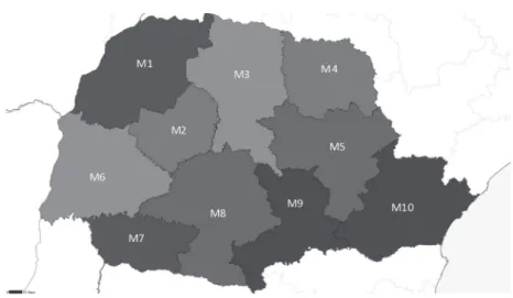
Figure 1. Mesoregions in Paraná State
Source: Results of the study.
asymmetrical distribution to the data. In this context if the asymmetry is negative, then the probability of loss will be underestimated in relation to the true distribution. The opposite is also true.
4. Data description
The municipality-level soybean yield data were acquired from the Secretary of Agriculture of the State of Parana (Seab), from 1981 to 2007, in kg/hectare. The municipality-level yield is an average for crop yield in the municipality and is based on the subjective methodology created by the Geography and Statistics Brazilian Institute (IBGE). These statistics are based on a consensus among agricultural players in a municipality (farmers, bank managers, crop extensionists, etc). Thus, the IBGE releases the average yield for each municipality. Given a mesoregion, we select the minimum value of the soybean yield in a group of municipalities within the mesoregion. In other words, if there are ten mesoregions, we have ten observations in each year. This data are collected and released annually (two year lag).
Thus, the empirical application considers mesoregions (a set of municipalities) defined by the Brazilian Institute of Geography and Statistics (IBGE) (Figure 1). Considering the fact that in each mesoregion there exist a set of municipalities then the minimum value of this set of municipalities in a year is used to create the time series of minimum values for each mesoregion. We utilized this procedure for each year since 1980. Figure 2 shows the evolution of the average of the minimum values, from 1981 to 2007.
5. Results and discussion
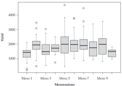
Table 1 and Figure 3 show, respectively, descriptive statistics and the boxplot of the soybean yield for all mesoregions. The descriptive statistics show that the median is systematically higher than average or smaller, which suggests that the distributions are asymmetric to the left or to the right, respectively.
Figure 2. Boxplot of the yields for each mesoregion
Meso 1 4000
3000
2000
1000
Meso 3 Meso 5
Mesoregions
Y
ield
Meso 7 Meso 9
Source: Results of the study.
Table 1. Soybean yield descriptive statistics
Mesoregion Number of
Counties Mean Median
Standard
Deviation Skewness
Excess
Kurtosis CV
M1 61 1302.5 1427 471.0 -0.487 -0.321 36,2
M2 25 1931.3 1941 626.3 0.146 0.051 32,4
M3 79 1639.9 1476 560.4 0.501 0.038 34,2
M4 46 1712.6 1712 373.4 -0.209 0.117 21,8
M5 14 2022.7 2000 974.2 0.827 0.019 48,2
M6 50 2006.7 1983 719.9 0.898 0.043 35,9
M7 37 2096.7 1907 752.8 1.279 1.741 35,9
M8 29 1769.1 1740 706.9 0.517 -0.794 40,0
M9 21 1968.8 1983 868.1 0.465 -1.003 44,1
M10 37 1383.7 1495 284.3 0.051 -1.501 20,5
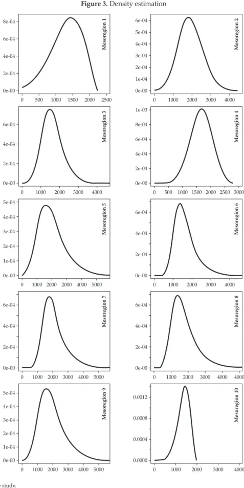
Figure 3. Density estimation
0 8e-04
6e-04
4e-04
2e-04
0e-00
500 1000 1500 2000 2500
Mesor
egion 1
0 1000 2000 3000 6e-04
5e-04
4e-04
3e-04
2e-04
1e-04
0e-00
4000
Mesor
egion 2
0 6e-04
4e-04
2e-04
0e-00
1000 2000 3000 4000
Mesor
egion 3
0 500 1000 1500 2000 3000 1e-03
8e-04
6e-04
4e-04
2e-04
0e-00
2500
Mesor
egion 4
0 5e-04
3e-04 4e-04
2e-04
1e-04
0e-00
1000 2000 2000 4000 5000
Mesor
egion 5
0 1000 2000 3000 6e-04
4e-04
2e-04
0e-00
4000
Mesor
egion 6
0 6e-04
4e-04
2e-04
0e-00
1000 2000 3000 4000 5000
Mesor
egion 7
0 1000 2000 3000 6e-04
4e-04
2e-04
0e-00
4000 4000
Mesor
egion 8
0 5e-04
3e-04 4e-04
2e-04
1e-04
0e-00
1000 2000 3000 4000 5000
Mesor
egion 9
0 1000 2000 3000 0.0012
0.0008
0.0004
0.0000
4000
Mesor
egion 10
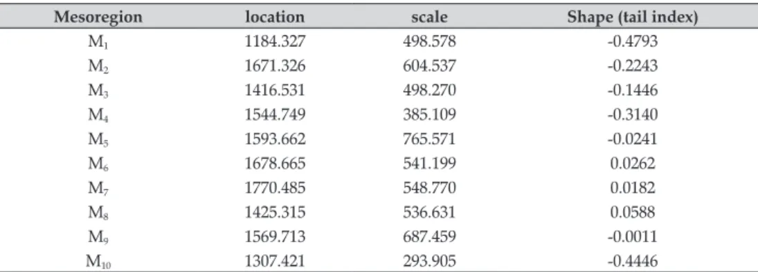
Table 2. Estimates of the location, scale and shape parameters
Mesoregion location scale Shape (tail index)
M1 1184.327 498.578 -0.4793
M2 1671.326 604.537 -0.2243
M3 1416.531 498.270 -0.1446
M4 1544.749 385.109 -0.3140
M5 1593.662 765.571 -0.0241
M6 1678.665 541.199 0.0262
M7 1770.485 548.770 0.0182
M8 1425.315 536.631 0.0588
M9 1569.713 687.459 -0.0011
M10 1307.421 293.905 -0.4446
Source: Results of the study.
Table 3. Intervals of 95% confidence for the shape parameter (ξ) and values of the
Modified Likelihood Ratio Test (T* LR)
Mesoregion
Limits of 95% confidence intervals for ξ
(T*
LR) Distribution
Lower Upper
M1 -0.721 -0.211 10.240 Weibull
M2 -0.421 0.003 3.783 Gumbel
M3 -0.382 0.093 1.353 Gumbel
M4 -0.545 -0.123 5.975 Weibull
M5 -0.288 0.248 0.032 Gumbel
M6 -0.294 0.346 0.030 Gumbel
M7 -0.207 0.243 0.026 Gumbel
M8 -0.496 0.554 0.082 Gumbel
M9 -0.571 0.471 0.001 Gumbel
M10 -0.961 0.073 0.030 Gumbel
Source: Results of the study.
Table 2 shows the point estimates of the
shape parameter ξ 1 α
= . Results show that the
shape parameters were negative for 7 regions and positive for 3 regions suggesting that the extreme distributions are either Weibull or Gumbel.
Comparing the value of the statistics T* LR
^ h
presented in Table 3 with the χ2 statistics with one
degree of freedom and 5% level of significance .
3 84
; .
1 0 05 2
χ =
^ h, one can note that the distribution
to be fitted is the Gumbel distribution in the mesoregions 2, 3, 5, 6, 7, 8, 9 and 10. On the other side the mesoregions 1 and 4 will be modeled using the Weibull distribution. This fact
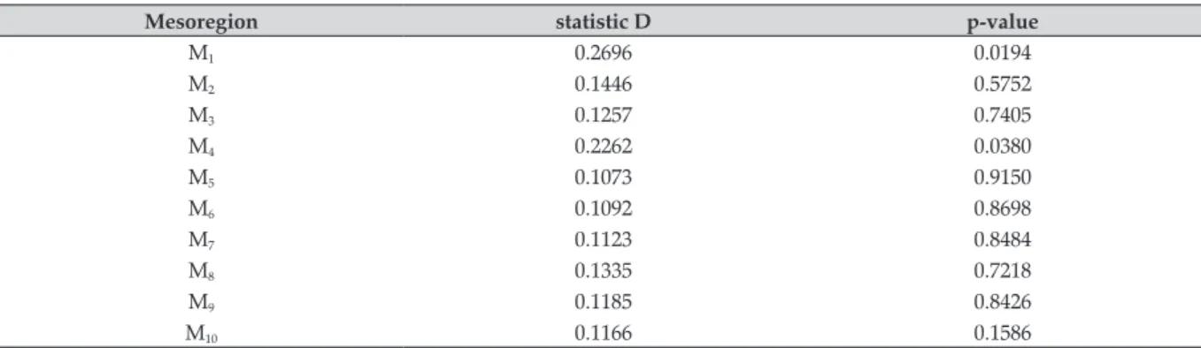
is confirmed by the D statistics (Kolmogorov-Smirnov test)presented in Table 3. According to the test most of the mesoregions could be fitted by the Gumbel distribution.
Table 4. Shapiro-Wilk normality test
Mesoregion statistic W p-value
M1 0.9653 0.0483
M2 0.9751 0.7390
M3 0.9662 0.5044
M4 0.9775 0.8012
M5 0.9385 0.0121
M6 0.9159 0.0314
M7 0.8904 0.0081
M8 0.9334 0.0837
M9 0.9205 0.0404
M10 0.9092 0.0218
Source: Results of the study.
Table 5. Kolmogorov-Smirnov test – diagnostic of the fitted distribution (Gumbel)
Mesoregion statistic D p-value
M1 0.2696 0.0194
M2 0.1446 0.5752
M3 0.1257 0.7405
M4 0.2262 0.0380
M5 0.1073 0.9150
M6 0.1092 0.8698
M7 0.1123 0.8484
M8 0.1335 0.7218
M9 0.1185 0.8426
M10 0.1166 0.1586
Source: Results of the study.
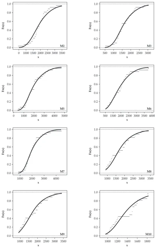
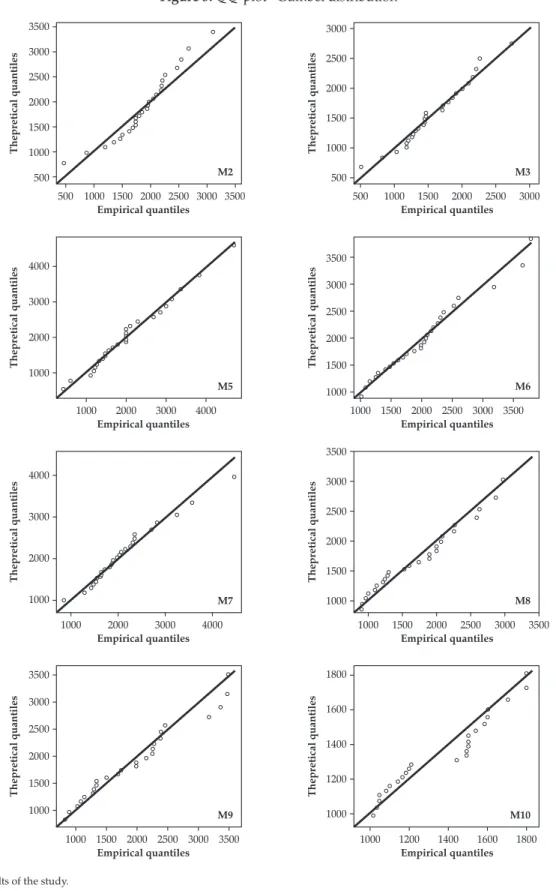
Figure 4 shows the distributions adjusted for each mesoregion. Most of the distributions are asymmetric to the right. In this context, the probability of loss is supposed to be higher compared to the Normal distribution case, commonly used by the insurance companies. The Figure 5 shows the diagnostics of the fitted distribution through the qq-plot. Considering the level of significance of 1%, Table 4 shows that the
data follow the GEV distribution. In other words, the null hypothesis cannot be rejected.
Figure 4. Kolgomorov-Sminorv test of the empirical cumulative distribution (dotted line) and theoretical distribution (continuous line)
0 0.8 1.0
0.6
Fn(x) Fn(x)
0.2 0.4
0.0
0.8 1.0
0.6
0.2 0.4
0.0 1000 2000
x x
1500 250030003500
M3 M2
500 1000 1500 2000 2500 3000
0 0.8 1.0
0.6
Fn(x) Fn(x)
0.2 0.4
0.0
0.8 1.0
0.6
0.2 0.4
0.0 1000 3000
x x
2000 4000 5000
M6 M5
500 1500 2000 2500 30003500 4000
0.8 1.0
0.6
Fn(x) Fn(x)
0.2 0.4
0.0
0.8 1.0
0.6
0.2 0.4
0.0 1000 3000
x x
2000 4000
M8 M7
1000 1500 2000 2500 3000 3500
0.8 1.0
0.6
Fn(x) Fn(x)
0.2 0.4
0.0
0.8 1.0
0.6
0.2 0.4
0.0 1000 2000
x x
1500 2500 3000 3500
M10 M9
1000 1200 1400 1600 1800
Figure 5. QQ-plot –Gumbel distribution
500 2500 3000 3500
2000
Thepr
etical quantiles
Thepr
etical quantiles
1000 1500
500
2500 3000
2000
1000 1500
500
1000 2000
Empirical quantiles Empirical quantiles 1500 2500 3000 3500
M3 M2
500 1000 1500 2000 2500 3000
4000
Thepr
etical quantiles
Thepr
etical quantiles
2000 3000
1000
3000 3500
2500
1500 2000
1000 1000 3000
Empirical quantiles Empirical quantiles 2000 4000
M6 M5
1000 1500 2000 2500 3000 3500
4000
Thepr
etical quantiles
Thepr
etical quantiles
2000 3000
1000
3000 3500
2500
1500 2000
1000
1000 3000
Empirical quantiles Empirical quantiles 2000 4000
M8 M7
1000 1500 2000 2500 3000 3500
3000 3500
2500
Thepr
etical quantiles
Thepr
etical quantiles
1500 2000
1000
1800
1600
1200 1400
1000
1000 2000
Empirical quantiles Empirical quantiles 1500 2500 3000 3500
M10 M9
1000 1200 1400 1600 1800
Table 6. Probability of loss assuming the Weibull and Gumbel distributions – levels of coverage of 60, 70 and 80%
Mesoregion Level of coverage (ϑ)
60% 70% 80%
M1 13.8 19.7 27.1
M2 11.4 19.3 29.3
M3 10.4 18.6 29.2
M4 4.7 11.0 21.7
M5 19.4 28.3 38.0
M6 8.8 18.9 31.8
M7 7.7 17.5 30.6
M8 13.6 24.1 36.1
M9 17.2 26.7 37.1
M10 3.4 7.9 16.3
Source: Results of the study.
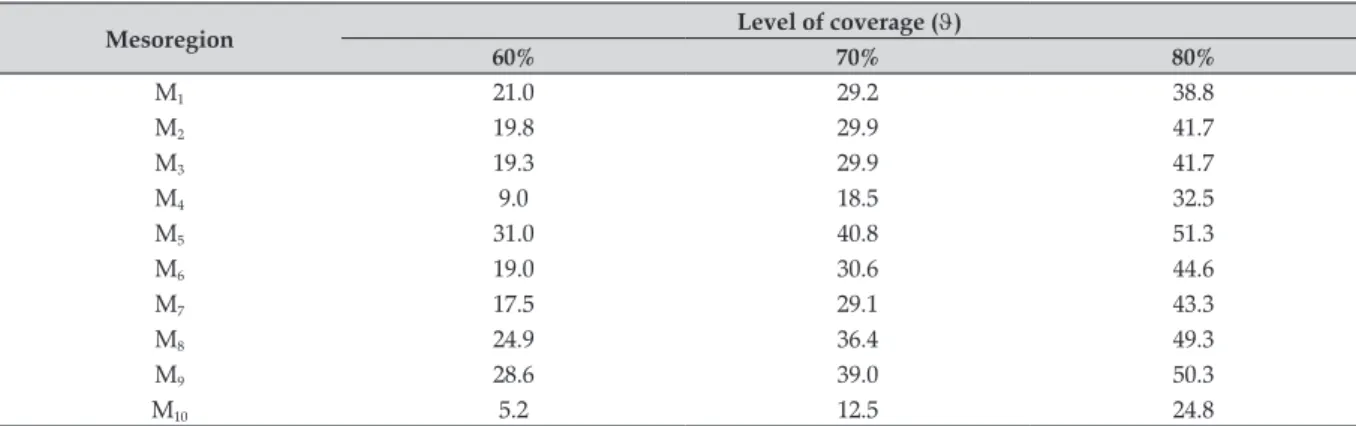
Table 7. Probability of loss assuming the Normal distribution - levels of coverage of 60, 70, and 80%
Mesoregion Level of coverage (ϑ)
60% 70% 80%
M1 21.0 29.2 38.8
M2 19.8 29.9 41.7
M3 19.3 29.9 41.7
M4 9.0 18.5 32.5
M5 31.0 40.8 51.3
M6 19.0 30.6 44.6
M7 17.5 29.1 43.3
M8 24.9 36.4 49.3
M9 28.6 39.0 50.3
M10 5.2 12.5 24.8
Source: Results of the study.
One must note that the level of coverage is a parameter chosen by the insured at the beginning of the insurance contract. In this context, the agricultural producer can choose the levels from 60 to 80% of the average yield of the municipality i (μi) resulting in the critical yield. If the final yield - in the end of the harvest, yi, is
lesser than the critical, the insured receives the indemnity. In this study, because of the fact that we aggregate the information into mesoregions, the critical yield is related to each mesoregion instead of municipalities. Thus, the premium rate is calculated for each mesoregion.
In Tables 5 and 6 one can notice that for all levels of coverage, the probability of loss estimated using the Normal distribution is greater than the
distributions. A direct implication of this fact is the overpricing of the premium rate, given by (Goodwin and Ker, 1998):
|
Pr emium Rate F E Y y<
Y Y
αµ
αµ αµ αµ =
−
^ h 6 ^ h@
in which E is the expectation operator and F is the distribution function.
The probability of loss is represented by the distribution function in the premium rate formulae. In the calculation of the rate, the operator of expectation and the term in the denominator are constant.
3,18%, respectively, considering the distributions Weibull and Normal.
In the insurance market this difference represents a large variation in the total premium. Considering for example, that a insurance company sells to a soybean producer a insurance contract in the Mesoregion 1 charging 3,18% (Normal rate) instead of 2% (Weibull rate). Suppose, for instance, the average liability is equal to US$ 1 mi in a pool (20 thousand producers). The average premium charged is approximately US$ 31,800 instead of US$ 20,000. The soybean producers will be overcharged on average in US$ 11,800 and US$ 236 mi, in total.
6. Conclusion
In this research we analysed alternative statistical assumptions for estimating the probability of loss with SEAB’s agricultural yield data and analyse its consequences in the premium rate. The soybean data were adjusted considering the Weibull-Gumbel and Normal distributions for all mesoregions in Paraná state.
Moreover, the probability of loss in Table 5 is quite different from the results in Table 6. The normality assumption is commonly used by most of the crop insurance companies in Brazil because of its mathematical tractability. Looking more carefully at the results, for all levels of coverage, the probabilities of loss are higher in the Normal case. On average, 77, 54 and 41% for the 60, 70 and 80% level of coverage, respectively.
It means that insurance companies are ignoring the skewness of the distribution and overpricing the risk. The pure premium rate is actually smaller than the premium rate charged. The consequence for the insurance market is that high risk producers may find attractable to demand the insurance increasing the probability to receive the indemnity. This classical problem, known as adverse selection, is well documented in the economical and actuarial literature and it could cause severe problems of financial losses in the agricultural insurance market.
From the insurance company point of view, supposing a Normal distribution, the probability of loss is greater than the rate estimated using the Weibull-Gumbel distributions. It means that if the true distribution is non-symmetric then the Normal case will overestimate the true rate. When the crop insurance is not compulsory, higher rates implies that the insurance company will adversely select only the farmers with higher risks. Otherwise, when the crop insurance is compulsory, the insurance company increases their revenue by charging a higher premium rate dissatisfying the farmer. However, in this situation, by spreading out the crop insurance in several regions the risk is better managed by the insurance company. On the other hand if the true distribution is symmetric than the Normal distribution could be used to estimate the premium rate. In this case, estimating the rates by the Weibull-Gumbel distributions will underestimate the rates. Farmers will be undercharged and the insurance companies will lose revenue.
In a market where historically most of the producers avoid demanding insurance products because of its high premium rate, and high probability to have indemnities paid higher than premiums collected by insurers, better statistical assumptions should be taking into account to better reflect the agricultural risk and the calculation of the premium rate.
7. References
ATWOOD, J., SHAIK, S. and WATTS, M. Are crop yields normally distributed? A reexamination. American
Journal of Agricultural Economics, v. 85, p. 888-901, 2003.
BABCOCK, B. A., HART, C. E. and HAYES, D. J. Actuarial fairness of crop insurance rates with constant
rate relativities. American Journal of Agricultural
Economics, v. 86, p. 563-575, 2004.
BAUTISTA, E. A. L., ZOCCHI, S. S. and ANGELOCCI, L. R. A distribuição generalizada de valores extremos aplicada ao ajuste dos dados de velocidade máxima
de vento em Piracicaba, SP. Revista de Matemática e
CARTWRIGHT, D. E. On estimating the mean energy of sea waves from the highest waves in a record.
Proceedings of the Royal Society of London, v. 247, p. 22-28, 1958.
COBLE, K. H., KNIGHT, T. O., POPE, R. D. and WILLIAMS, J. R. An expected indemnity approach to the measurement of moral hazard in crop insurance.
American Journal of Agricultural Economics, v. 79, p. 216-26, 1997.
DANIELSSON, J. and VRIES, C. de. Value-at-Risk and extreme returns. Annales d’Economie et de Statistique, v. 60, p. 239-270, 2000.
DAY, R. H. Probability distributions of field crop yields.
Journal of Farm Economics, v. 47, p. 713-741, 1965.
DIEBOLD, F. X., SCHUERMANN, T. and STROUGHAIR, J. D. Pitfalls and opportunities in the use of extreme value theory in risk management. In: REFENES, A. P., A. BURGESS and J. MOODY (Ed.).
Decision Technologies for Computational Finance, Kluwer Academic Publishers, 1998.
EMBRECHTS, P., KLÜPPELBERG, C. and MIKOSCH, T. Modelling extremal events for insurance and finance. Spring Verlag, Berlin, 1997.
FISHER, R. A. and TIPPETT, L. H. C. Limiting forms of the frequency distribution of the largest and smallest member of a sample, Proc. Cambridge Phil. Soc., v. 24, p. 180-190, 1928.
GALLAGHER, P. U.S. Soybean yields: estimation and forecasting with nonsymmetric disturbances. American Journal of Agricultural Economics, v. 69, p. 796-803, 1987.
GENCAY, R., SELCUK, F. and ULUGÄULYAGCI, A. High volatility, thick tailsand extreme value theory in value-at-risk estimation. Insurance: Mathematics and Economics, v. 33, p. 337-356, 2003.
GOODWIN, B. K. and KER, A. P. Nonparametric estimation of crop yield distributions: implications for rating group-risk crop insurance contracts. American Journal of Agricultural Economics, v. 80, p. 139-153, 1998.
GOODWIN, B. K., ROBERTS, M. C. and COBLE, K. H. Measurement of price risk in revenue insurance: implications of distributional assumptions. Journal of Agricultural and Resource Economics, v. 25, p. 195-214, 2000.
HOSKING, J. R. M., WALLIS, J. R. and WOOD, E. F. Estimation of the generalized extreme value distribution by the method of probability-weighted moments. Technometrics, Alexandria, v. 27, p. 251-261,
DE HAAN, L. and PEREIRA, A. E. Spatial extremes: Models for the stationary case. Annals of Statistics, Philadelphia, v. 34, p. 146-168, 2006.
JUST, R.E. and WENINGER, Q. Are crop yields normally distributed? American Journal of Agricultural Economics, v. 81, p. 287-304, 1999.
KOEDIJK, K. G., SCHAFGANS, M. and VRIES, C. de. The tail index of exchange rate returns. Journal of International Economics, v. 29, p. 93-108, 1990.
LONGIN, F. M. The assymptotic distribution of extreme stock market returns. Journal of Business, v. 69, p. 383-408, 1996.
LORETAN, M. and PHILLIPS, P. Testing the covariance
stationarity ofheavy-tailed time series. Journal of
Empirical Finance, v. 1, p. 211-248, 1994.
MCNEIL, A. J. and FREY, R. Estimation of tail-related risk measures for heteroscedastic financial time series: an extreme value approach. Journal of Empirical Finance, v. 7, p. 271-300, 2000.
MOSS, C. B. and SHONKWILER, J. S. Estimating yield distributions with a stochastic trend and non Normal errors. American Journal of Agricultural Economics, v. 75, p. 1056-1062, 1993.
NEFTCI, S. N. Value at risk calculations, extreme events, and tail estimation. Journal of Derivatives, p. 23-37, 2000.
NELSON, C. H. and PRECKEL, P. V. The conditional beta distribution as a stochastic production function.
American Journal of Agricultural Economics, v. 71, p. 370-378, 1989.
NEWELL, G. F. Asymptotic extremes for m-dependent random variables. Annals of Mathematical Statistics, v. 35, p. 1322-1325, 1964.
O’BRIEN, G. L. Limit theorems for the maximum term of a stationary process. Annals of Probability, v. 2, p. 540-545, 1974.
OZAKI, V. A. and SILVA, R. S. Bayesian ratemaking procedure of crop insurance contracts with skewed distribution. Journal of Applied Statistics, v. 36, p. 443-452, 2009.
OZAKI, V. A. A digression about the subvention program for rural insurance premium and the implications for the future of the rural insurance market. Brazilian Review of Risk and Insurance, v. 2, p. 79-94, 2008.
RAMIREZ, O. A. Estimation and use of a multivariate parametric model for simulating heteroskedastic, correlated, nonNormal random variables: the case of
corn belt corn, soybean and wheat yields. American
Journal of Agricultural Economics, v. 79, 191-205, 1997.
RAMIREZ, O. A., MISRA, S. and FIELD, J. Crop-yield distributions revisited, American Journal of Agricultural Economics, v. 85, p. 108-120, 2003.
SANSIGOLO, C. A. A distribuição de extremos e precipitação diária, temperatura máxima e mínima
e velocidade do vento em Piracicaba, SP (1917-2006).
Revista de Matemática e Estatística, v. 23, p. 341-346, 2008.
TAYLOR, C. R. Two practical procedures for estimating multivariate nonNormal probability density functions.
American Journal of Agricultural Economics, v. 72, p. 210-217, 1990.