Initiation of a Marinoan Snowball Earth in a state-of-the-art atmosphere-ocean general circulation model

(1)

CPD

6, 1853–1894, 2010

Marinoan Snowball Earth

A. Voigt et al.

Title Page

Abstract Introduction

Conclusions References

Tables Figures

◭ ◮

Back Close

Full Screen / Esc

Printer-friendly Version Interactive Discussion

Discussion

P

a

per

|

Dis

cussion

P

a

per

|

Discussion

P

a

per

|

Discussio

n

P

a

per

|

Clim. Past Discuss., 6, 1853–1894, 2010 www.clim-past-discuss.net/6/1853/2010/ doi:10.5194/cpd-6-1853-2010

Climate of the Past Discussions

This discussion paper is/has been under review for the journal Climate of the Past (CP). Please refer to the corresponding final paper in CP if available.

Initiation of a Marinoan Snowball Earth in

a state-of-the-art atmosphere-ocean

general circulation model

A. Voigt1,2, D. S. Abbot3, R. T. Pierrehumbert3, and J. Marotzke1

1

Max Planck Institute for Meteorology, Hamburg, Germany

2

International Max Planck Research School on Earth System Modelling, Hamburg, Germany

3

Department of Geophysical Sciences, University of Chicago, Chicago, Illinois, USA

Received: 9 September 2010 – Accepted: 21 September 2010 – Published: 23 September 2010

Correspondence to: A. Voigt (aiko.voigt@zmaw.de)

(2)

CPD

6, 1853–1894, 2010

A. Voigt et al.

Title Page

Tables Figures

◭ ◮

Back Close

Full Screen / Esc

Discussion

P

a

per

|

Dis

cussion

P

a

per

|

Discussion

P

a

per

|

Discussio

n

P

a

per

|

Abstract

We study the initiation of a Marinoan Snowball Earth (635 million years before present) with the most sophisticated atmosphere-ocean general circulation model ever used for this purpose, ECHAM5/MPI-OM. A comparison with a pre-industrial control climate shows that the change of surface boundary conditions from present-day to Marinoan, 5

including a shift of continents to low latitudes, induces a global mean cooling of 4.6 K. Two thirds of this cooling can be attributed to increased planetary albedo, the remaining one third to a weaker greenhouse effect. The Marinoan Snowball Earth bifurcation point for pre-industrial atmospheric carbon dioxide is between 95.5 and 96% of the present-day total solar irradiance (TSI), whereas a previous study with the same model 10

found that it was between 91 and 94% for present-day surface boundary conditions. A Snowball Earth for TSI set to its Marinoan value (94% of the present-day TSI) is prevented by quadrupling carbon dioxide with respect to its pre-industrial level. A zero-dimensional energy balance model is used to predict the Snowball Earth bifurcation point from only the equilibrium global mean ocean potential temperature for present-15

day TSI. We do not find stable states with sea-ice cover above 55%, and land conditions are such that glaciers could not grow with sea-ice cover of 55%. Therefore, none of our simulations qualifies as a “slushball” solution. In summary, our results contradict previous claims that Snowball Earth initiation would require “extreme” forcings.

1 Introduction

20

The apparent existence of low-latitude land glaciers at sea level during at least two episodes of the Neoproterozoic era, the Sturtian (∼710 million years before present, Ma) and the Marinoan (∼635 Ma) (Evans, 2000; Trindade and Macouin, 2007; Mac-donald et al., 2010), has led to the proposal that these glaciations were accompa-nied by completely ice-covered oceans. This so-called “Snowball Earth” hypothesis 25

(3)

CPD

6, 1853–1894, 2010

A. Voigt et al.

Title Page

Tables Figures

◭ ◮

Back Close

Full Screen / Esc

Discussion

P

a

per

|

Dis

cussion

P

a

per

|

Discussion

P

a

per

|

Discussio

n

P

a

per

|

formations and cap carbonates (Hoffman and Schrag, 2002), has not only attracted the attention of geologists, but also of climate modellers, who have tested if the Snowball Earth hypothesis is compatible with climate physics.

The Snowball Earth hypothesis itself relies on a runaway ice-albedo feedback first reported in energy balance models (e.g., Budyko, 1969; Sellers, 1969). After the initial 5

perception that the Snowball Earth hypothesis is, in principle, compatible with climate physics, the last decade has seen the full hierarchy of climate models being applied to Snowball Earth initiation. While we do not know of any climate model that excludes Snowball Earth solutions categorically, various climate modelling studies concluded that completely ice-covered oceans require “extreme” forcings (Chandler and Sohl, 10

2000; Poulsen et al., 2001; Poulsen, 2003; Poulsen and Jacob, 2004) that might be considered unrealistic for the Neoproterozoic. At the same time, Hyde et al. (2000) and Peltier et al. (2004), using an energy balance model with interactive ice sheets, found so-called “Slushball Earth” or “oasis” solutions in which tropical land glaciers can coexist with large areas of perennially open tropical water. Despite severe limitations 15

of their model, including the disregard of atmosphere and ocean dynamics, these so-lutions were supported by an atmospheric general circulation model coupled to a slab ocean and prescribed full continental glaciation (Hyde et al., 2000; Baum and Crow-ley, 2001). Moreover, Chandler and Sohl (2000) and Micheels and Montenari (2008) found, also using atmospheric general circulation models coupled to slab oceans, so-20

lutions with equatorial land masses below freezing in conjunction with almost but not completely ice-covered oceans. As a result, the apparent difficulties in freezing the en-tire ocean combined with the possibility that equatorial land glaciers might not require completely ice-covered oceans has evoked the impression that the Snowball Earth hy-pothesis is implausible from the perspective of climate modelling. As a consequence 25

attention shifted to the Slushball Earth hypothesis (Lubick, 2002; Kaufman, 2007; Kerr, 2010).

(4)

CPD

6, 1853–1894, 2010

A. Voigt et al.

Title Page

Tables Figures

◭ ◮

Back Close

Full Screen / Esc

Discussion

P

a

per

|

Dis

cussion

P

a

per

|

Discussion

P

a

per

|

Discussio

n

P

a

per

|

boundary conditions, for which most of the continents are at low latitudes. We investi-gate the total solar irradiance (TSI) and atmospheric CO₂ concentration that cause a Snowball Earth bifurcation as well as the maximum stable sea-ice cover. Our climate model incorporates physics found to be essential for Snowball Earth initiation, including ocean dynamics (Poulsen et al., 2001; Poulsen and Jacob, 2004), sea-ice dynamics 5

(Lewis et al., 2003, 2007) and clouds (Poulsen and Jacob, 2004). Note that to date, there is no model that supports the Slushball Earth hypothesis and incorporates all of the above physics. By comparing the simulations to a previous study with this model for present-day surface boundary conditions (Voigt and Marotzke, 2009), we also reevalu-ate if low-latitude continents favor Snowball Earth initiation as suggested by Kirschvink 10

(1992).

The paper is organised as follows. Section 2 describes the climate model, the Marinoan surface boundary conditions, and the setup of the ECHAM5/MPI-OM sim-ulations. Section 3 analyzes the Marinoan control climate and compares it to a pre-industrial control simulation by means of a one-dimensional energy balance model of 15

zonal mean surface temperature. This enables us to investigate the climatic effect of changing surface boundary conditions form present-day to Marinoan. Section 4 in-vestigates the Snowball Earth bifurcation point and maximum stable sea-ice cover. A zero-dimensional energy balance model of global mean ocean potential temperature is used to predict the Snowball Earth bifurcation point in Sect. 5. Section 6 gives a gen-20

(5)

CPD

6, 1853–1894, 2010

A. Voigt et al.

Title Page

Tables Figures

◭ ◮

Back Close

Full Screen / Esc

Discussion

P

a

per

|

Dis

cussion

P

a

per

|

Discussion

P

a

per

|

Discussio

n

P

a

per

|

2 Model and simulation setup

2.1 Model setup

We apply the state-of-the-art atmosphere-ocean general circulation model ECHAM5/MPI-OM. This is the same model that was used to study the transition to a modern Snowball Earth (Voigt and Marotzke, 2009), apart from technical changes 5

to adapt the model to the new supercomputer of the German Climate Computing Center (DKRZ). ECHAM5/MPI-OM ranks among the world’s top climate models (Reichler and Kim, 2008) and has been used for a variety of applications, ranging from climate projections for the Intergovernmental Panel on Climate Change (Solomon et al., 2007) to paleo-climate simulations of the Holocene and Eemian (Fischer and 10

Jungclaus, 2010) as well as the Paleocene/Eocene (Heinemann et al., 2009).

Comprehensive documentation of the atmosphere model ECHAM5 (we use version ECHAM5.3.02p) is given by Roeckner et al. (2003), details of the ocean model MPI-OM (here used in version 1.2.3p2) are described by Marsland et al. (2003). We here only review the model features and boundary conditions that are salient to our study 15

and its comparison to previous Snowball Earth initiation studies.

Our Marinoan continents follow the reconstruction of M. Macouin (pers. comm.) and are similar to, though less dispersed than, the continents used by Le Hir et al. (2009) (Fig. 1). In contrast to today, landmasses are largely clustered from 45◦S to 30◦N with two large equatorial continents separated by a narrow seaway. Zonal mean land 20

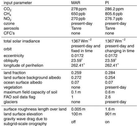
fraction from 60◦S to 20◦N is higher in the Marinoan than today, with the majority of the Marinoan landmasses located in the Southern Hemisphere Fig. (2). We set land surface albedo to 0.272 globally (see Table 1). This value is chosen such that the global mean background surface albedo (zero sea-ice and snow cover) of the Marinoan setup equals that of the present-day setup. This land albedo is close to the surface albedo of 25

(6)

CPD

6, 1853–1894, 2010

A. Voigt et al.

Title Page

Tables Figures

◭ ◮

Back Close

Full Screen / Esc

Discussion

P

a

per

|

Dis

cussion

P

a

per

|

Discussion

P

a

per

|

Discussio

n

P

a

per

|

length and soil-water holding capacity are specified to bare desert values of 5×10−3m and 0.1 m, respectively (Hagemann, 2002).

The presence of snow increases land surface albedo according to the fractional snow cover of the grid cell. Land snow albedo depends on surface temperature and ranges from 0.3 at 0◦C to 0.8 at or below −5◦C. Ocean surface albedo is set to 0.07. Bare 5

sea-ice albedo depends on sea-ice temperature and ranges from 0.55 at 0◦C to 0.75 at or below−1◦C. Snow on sea ice leads to the following albedo increase: if the water equivalent of snow depth is larger than 0.01 m, sea ice is treated as snow-covered. The albedo of snow-covered sea ice depends on snow surface temperature and ranges from 0.65 at 0◦C to 0.8 at or below −1◦C. The surface albedo of mixed grid cells is 10

calculated as an area fraction-weighted average of land, ocean, and sea-ice albedo. The sea-ice model follows the dynamics of Hibler (1979) while the thermodynamics are incorporated by a zero-layer Semtner model that relates changes in sea-ice thickness to a balance of radiative, turbulent, and oceanic heat fluxes (Semtner, 1976). The freezing point of sea water is fixed to−1.9◦C independent of salinity. Snow on ice is 15

explicitly modeled, including snow/ice transformation when the snow/ice interface sinks below the sea level because of snow loading. The effect of ice formation and melting is accounted for by assuming a sea-ice salinity of 5 psu. The sea-ice thickness is limited to about 8 m.

Orbital parameters are constant in time and correspond to year 800 A.D. Ozone 20

follows the 1980–1991 climatology of Fortuin and Kelder (1998), aerosols are pre-scribed according to Tanr ´e et al. (1984). Greenhouse gas concentrations are set to pre-industrial levels (CO2=278 ppm, CH4=650 ppb, N2O=270 ppb, no cfc). Lacking information on Marinoan orography we set land surface elevation to 100 m everywhere, implying that ECHAM5’s parametrization of gravity wave drag due to subgrid-scale 25

(7)

CPD

6, 1853–1894, 2010

A. Voigt et al.

Title Page

Tables Figures

◭ ◮

Back Close

Full Screen / Esc

Discussion

P

a

per

|

Dis

cussion

P

a

per

|

Discussion

P

a

per

|

Discussio

n

P

a

per

|

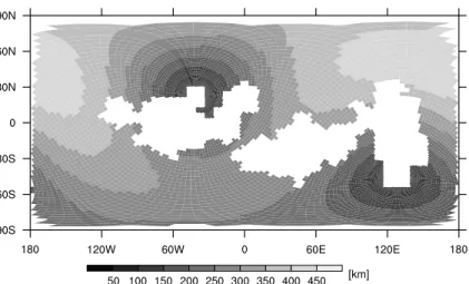
For the atmosphere model, ECHAM5, horizontal resolution is set to spectral trunca-tion T31 (∼3.75◦). In the vertical, 19 hybridσ-levels that extend up to 10 hPa are em-ployed. The time step is 2400 s. The ocean model MPI-OM applies a curvilinear grid with 114x106 points and poles over the two continents (51◦W/23◦N and 128◦E/46◦S), resulting in high horizontal resolution with grid distances smaller than 50 km near the 5

grid’s poles but low resolution with grid distances up to 435 km in parts of the Northern Hemisphere (Fig. 3). We use 39 vertical levels, with the top level having a thickness of 22 m. The time step is 5760 s. Some simulations required a reduced time step of 3600 s to overcome numerical instabilities (see Table 2). Marinoan ocean bathymetry is set to 5000 m globally. The atmosphere and ocean models are coupled via the OASIS3 10

coupler (Valcke et al., 2003) with a coupling time step of one day. No flux adjustments are applied.

We initialize ECHAM5/MPI-OM from warm atmospheric conditions and a homoge-neous ocean at rest and at a potential temperature of 283 K and a salinity of 34.3 psu. The latter is approximately the salinity we would obtain in the present-day ocean if all 15

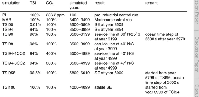
glaciers were melted completely (Heinemann et al., 2009). The model is then run to equilibrium at today’s total solar irradiance and pre-industrial greenhouse gas levels by integrating it for 3500 years. Years 3400 to 3499 serve as Marinoan control climate (MAR).

Simulations with reduced total solar irradiance, in some cases combined with an 20

increase of atmospheric carbon dioxide, are started from year 3499 of MAR (see Ta-ble 2). An additional simulation with total solar irradiance reduced to 95.5% (TSI955) is started from year 6199 of TSI96. Moreover, we perform one simulation where we set TSI back to 100% after complete sea-ice cover has been accomplished (TSI100). Throughout this study, years are counted with respect to model initialization at year 0. 25

(8)

CPD

6, 1853–1894, 2010

A. Voigt et al.

Title Page

Tables Figures

◭ ◮

Back Close

Full Screen / Esc

Discussion

P

a

per

|

Dis

cussion

P

a

per

|

Discussion

P

a

per

|

Discussio

n

P

a

per

|

on Myhre et al. (1998) we estimate that this causes a radiative forcing of−0.27 Wm−2 between PI and MAR, i.e., less than 0.1% of the global mean incident shortwave ra-diation at the top of the atmosphere. In what follows, we neglect this small e_ffect and discuss PI and MAR as if they employed the same concentrations of carbon dioxide, methane and nitrous oxide. Moreover, after the simulations have been completed we 5

have noticed that the Marinoan runs presented here use Pacanowski-Philander verti-cal viscosity and diffusivity parameters (Marsland et al., 2003) that are divided by five compared to the values used for the pre-industrial control run PI and the transition to a modern Snowball Earth (Voigt and Marotzke, 2009). Test runs have shown that the re-sults of this paper are robust with respect to this unintended parameter change (Voigt, 10

2010).

3 Marinoan control climate and comparison to the pre-industrial control climate

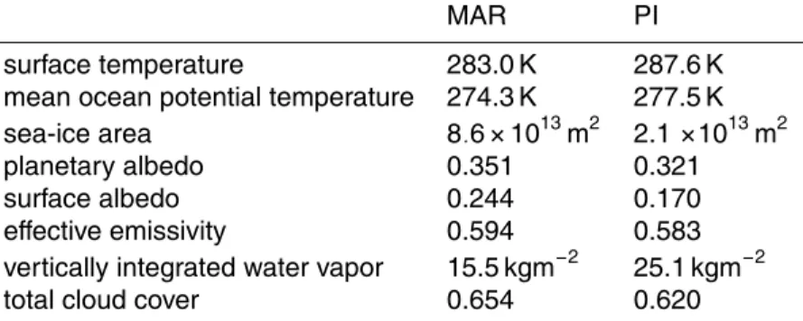
In this section, we describe the annual mean Marinoan control climate MAR and com-pare it to the annual mean pre-industrial control climate PI. Using a one-dimensional energy balance model we quantify how much of the cooling from PI to MAR is caused 15

by changes in albedo, effective emissivity (i.e., the greenhouse effect), and meridional heat transports.

3.1 Surface climate

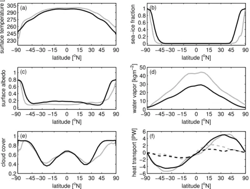
The Marinoan setup results in a global annual mean surface temperature of 283 K (Ta-ble 3). Zonal mean surface temperature is largely symmetric about the equator (Fig. 4), 20

(9)

CPD

6, 1853–1894, 2010

A. Voigt et al.

Title Page

Tables Figures

◭ ◮

Back Close

Full Screen / Esc

Discussion

P

a

per

|

Dis

cussion

P

a

per

|

Discussion

P

a

per

|

Discussio

n

P

a

per

|

than sea-surface temperatures, with annual mean surface temperatures of up to 302 K in the continents’ interior. Sea ice extends to 45◦N/S in the annual mean. Poleward of 70◦N/S, the ocean is covered with sea-ice year-round. Annual mean sea-ice thickness is less than 3 m equatorward of 70◦N/S, but as high as 7 m near the poles. Except very close to the annual mean sea-ice margin, sea ice is everywhere covered by snow 5

thicker than 0.01 m water equivalent. Most parts of the continents are snow-free; land snow-cover is restricted to the southernmost parts of the continents where snow depth reaches a water equivalent of 0.07 m at 133◦E/50◦S and of 0.02 m at 60◦E/52◦S. As expected from lower surface temperatures, the annual and zonal mean water vapor content is lower in MAR than in PI at all latitudes except close to the South Pole. Cloud 10

cover in MAR increases compared to PI in the tropics and poleward of 30◦N/S but decreases in the subtropics.

Atmospheric heat transport is larger in MAR than in PI in the tropics, accompanied by more vigorous Hadley cells, but smaller in SH midlatitudes due to reduced eddy transport. Poleward ocean heat transport is reduced in MAR compared to PI except 15

in SH midlatitudes. This change is reflected in the contribution of the meridional over-turning circulation which, for example, shows southward heat transport around 30◦N as a consequence of a strong anticlockwise (viewed from the East) Ekman cell that nearly reaches the ocean bottom (not shown). While a detailed analysis of MAR’s ocean circulation is not the aim of this study, we note that deep Ekman cells in the 20

absence of zonal boundaries have been reported in aquaplanet simulations with cou-pled atmosphere-ocean general circulation models before (Smith et al., 2006; Marshall et al., 2007). The deep Ekman cells result from vanishing zonal pressure gradient and largely zonally symmetric flow such that the return flow to the wind-generated merid-ional surface flow must be balanced by zonal momentum diffusion in the ocean interior 25

(10)

CPD

6, 1853–1894, 2010

A. Voigt et al.

Title Page

Tables Figures

◭ ◮

Back Close

Full Screen / Esc

Discussion

P

a

per

|

Dis

cussion

P

a

per

|

Discussion

P

a

per

|

Discussio

n

P

a

per

|

3.2 One-dimensional energy balance model

To gain quantitative insight into how changes in radiation and heat transport contribute to the differences between the Marinoan and pre-industrial control climates, we apply the one-dimensional energy balance model (1d-EBM) of zonal mean surface tempera-ture of Heinemann et al. (2009).

5

Assuming equilibrium and taking the zonal mean, net incoming shortwave radia-tion at the top of atmosphere (TOA) must be balanced by outgoing longwave radiaradia-tion (OLR) and divergence of meridional heat transport at each latitude (e.g., Stone, 1978). If we further parameterize OLR in terms of surface temperatureτ and effective emis-sivityǫ, we have

10

(1−α(φ))Q(φ)=σǫ(φ)τ4(φ)+H(φ), (1) whereα denotes planetary albedo,φ latitude, Q TOA incoming shortwave radiation,

σ=5.67×10−8Wm−2K−4the Stefan-Boltzmann constant, andH divergence of merid-ional heat transport. Quantities are understood as time and zonal mean values. Solving (1) forτyields the 1d-EBM estimate of surface temperature,τebm,

15

τebm(φ)≡τ(φ)=

4 s

1

σǫ(φ)

(1−α(φ))Q(φ)−H(φ)

, (2)

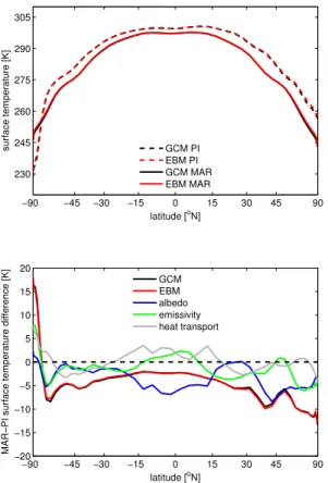
withα,Q,ǫ, and H diagnosed from the TOA and surface radiative fluxes of the GCM as described in Heinemann et al. (2009). The 1d-EBM’s surface temperature only marginally deviates from the GCM simulated surface temperature (see Fig. 5), with the error in the 1d-EBM’s surface temperature estimate caused by time and zonal varia-20

tions of surface temperature (Voigt, 2010).

(11)

CPD

6, 1853–1894, 2010

A. Voigt et al.

Title Page

Tables Figures

◭ ◮

Back Close

Full Screen / Esc

Discussion

P

a

per

|

Dis

cussion

P

a

per

|

Discussion

P

a

per

|

Discussio

n

P

a

per

|

effective emissivity, and meridional heat transport (note that incoming shortwave radi-ation at the top of atmosphere is the same in MAR and PI). Givenα,ǫ,andH for MAR and PI, the surface temperature difference between MAR and PI due to changes in planetary albedo is (Heinemann et al., 2009)

△τ(φ)

α

= 4 s

1

σǫ(φ_)PI

(1−α(φ_)MAR)Q(φ)−H_PI(φ)

−τ_ebmPI (φ).

5

The surface temperature changes resulting from changes inǫandH are estimated analogously.

Increased planetary albedo in MAR leads to a cooling compared to PI at all lati-tudes (Fig. 5). The only exception is the South Pole region where the replacement of high-topography the Antarctic ice sheet by sea ice results in a slight decrease of 10

surface albedo and thus a small planetary albedo warming effect. At most latitudes, the increased planetary albedo in MAR is caused by increased surface albedo through either increased sea-ice cover (poleward of 45◦N/S) or increased land fraction (45◦S to 20◦N). Between 20◦N and 45◦N, however, surface albedo in MAR is lower than in PI, showing that the increased planetary albedo in this region is due to increased cloud 15

cover (see Fig. 4e).

Outside the tropics, e_ffective emissivity in MAR mostly increases, leading to cooling in MAR compared to PI. This is consistent with a reduced atmospheric water vapor content causing a weaker greenhouse effect. In the tropics, however, effective emis-sivity decreases in MAR despite reduced tropical water vapor due to larger longwave 20

cloud radiative forcing (not shown). Heat transport changes from PI to MAR effect a warming in the tropics and a cooling in midlatitudes. This points at less total heat export from the tropics to midlatitudes (see Fig. 4f).

Finally, we quantify how the changes of planetary albedo, effective emissivity and heat transport contribute to the change of global mean surface temperature. This is 25

(12)

CPD

6, 1853–1894, 2010

A. Voigt et al.

Title Page

Tables Figures

◭ ◮

Back Close

Full Screen / Esc

Discussion

P

a

per

|

Dis

cussion

P

a

per

|

Discussion

P

a

per

|

Discussio

n

P

a

per

|

planetary albedo and the remaining one third by a weaker greenhouse effect through increased e_ffective emissivity. The global mean temperature change due to changes in the divergence of heat transport is negligible.

4 Snowball Earth bifurcation point and maximum stable sea-ice cover

This sections reports on the effect of an abrupt decrease of total solar irradiance and, 5

for some simulations, simultaneous increase of atmospheric carbon dioxide. These simulations enable us to find the Snowball Earth bifurcation point as well as the maxi-mum stable sea-ice cover.

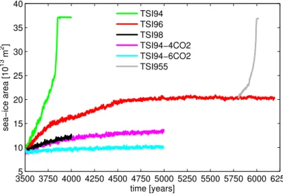
Virtually switching offthe sun results in global sea-ice cover within 9 years (simulation TSI00, not shown). A reduction of TSI to 94% of its present-day value leads to a 10

Snowball Earth within 355 years (simulation TSI94, see Fig. 6). In TSI94, the sea-ice line is nearly symmetric about the equator during the entire transition, and land snow accumulates in parts of the Southern Hemisphere but nowhere in the Northern Hemisphere. While surface albedo increases in the Northern Hemisphere are hence solely due to the conversion of open ocean areas to sea ice, snow accumulation on 15

land contributes to surface albedo increases in the Southern Hemisphere. The surface albedo of the Southern Hemisphere consequently increases at the same rate as the Northern Hemisphere surface albedo, and meridional heat transports stay symmetric about the equator during the entire transition (not shown). Moreover, it is worth noting that in a Snowball Earth state (years 3900 to 3999 of TSI94) annual-mean sea-ice 20

area is slightly below the global ocean area (the difference is less than 2% of the global ocean area) because some ocean regions are seasonally ice-free. However, before one puts trust in the realism of these seasonally sea-ice free regions, at least two model limitations would have to be fixed. First, sea-ice would likely grow much thicker if the model’s restriction of sea-ice thickness (see Sect. 2.1) was be removed. 25

(13)

CPD

6, 1853–1894, 2010

A. Voigt et al.

Title Page

Tables Figures

◭ ◮

Back Close

Full Screen / Esc

Discussion

P

a

per

|

Dis

cussion

P

a

per

|

Discussion

P

a

per

|

Discussio

n

P

a

per

|

temperatures. This permits unrealistic day-time melting of sea ice (Abbot et al., 2010) and potentially contributes to the simulation of seasonally ice-free ocean regions in a Snowball Earth state.

In contrast to a reduction of TSI to 94%, decreasing TSI to 96% does not cause global sea-ice cover (simulation TSI96). Sea-ice expansion in this simulation is initially 5

almost as fast as for a TSI reduction to 94%, but decelerates 250 years after the TSI decrease. A further 1000 years later, sea-ice area stabilizes at 20×1013m2, equivalent to 55% of the Marinoan ocean surface area.

To further pin down the Marinoan Snowball Earth bifurcation point, we branch off

simulation TSI955 from year 5799 of TSI96. In this simulation, total solar irradiance is 10

additionally decreased by 6.8 Wm−2 to 95.5% of its present-day value. This small ad-ditional TSI reduction is sufficient to induce global sea-ice cover within 201 years. The Snowball Earth bifurcation point, for pre-industrial carbon dioxide, therefore is between 95.5 and 96% of the present-day total solar irradiance.

The fact that we are able to fix the Snowball Earth bifurcation within an uncertainty of 15

0.5% of the present-day TSI also enables us to infer the maximum stable sea-ice cover. As shown by TSI96, sea ice can cover 55% of the ocean surface area without triggering a Snowball Earth instability. At the end of TSI96, the sea-ice line has stabilized at 30◦N and around 25◦S, respectively (Fig. 7), with sea ice being snow-covered except very close to the sea-ice edge, and snow on land restricted to largely thin snow cover in 20

the southernmost continental regions. The strong sensitivity of this sea-ice line to the small reduction in TSI demonstrates that in ECHAM5/MPI-OM, equilibrium solutions with sea-ice cover above 55% are highly unlikely, or if they occur, highly unstable.

Falling into a Snowball Earth when TSI is reduced to 94% can be prevented by an appropriate increase in atmospheric carbon dioxide. Combining a reduction of TSI to 25

(14)

CPD

6, 1853–1894, 2010

A. Voigt et al.

Title Page

Tables Figures

◭ ◮

Back Close

Full Screen / Esc

Discussion

P

a

per

|

Dis

cussion

P

a

per

|

Discussion

P

a

per

|

Discussio

n

P

a

per

|

Marinoan (Pierrehumbert, 2010; Gough, 1981), the Snowball Earth bifurcation is be-tween one and four times the pre-industrial level of carbon dioxide. Increasing carbon dioxide even further to 6 times its pre-industrial level almost compensates for the de-crease of TSI to 94% (simulation TSI94-6CO2). After 1000 years, sea-ice area in this simulation is only slightly higher than in the control simulation MAR.

5

Reducing TSI to 94% and quadrupling carbon dioxide has almost the same effect on sea-ice area as reducing TSI to 98%. This is consistent with the fact that the radiative forcing of increasing TSI by 4% (assuming a planetary albedo of 0.353 as simulated for MAR),

RF(4%TSI₀)=(1−0.353)·0.041367 4 Wm

−2

=8.8 Wm−2,

10

is close to the radiative forcing of quadrupling carbon dioxide (Myhre et al., 1998),

RF(4×CO2)=5.35ln4 Wm−2=7.4 Wm−2.

Note that if we took into account that the planetary albedo increases in the course of TSI98 and TSI94-4CO2, we would obtain a lower radiative forcing estimate for the 4% reduction in TSI, bringing the two estimates slightly closer together. Moreover, the 15

factor of 5.35 used in the radiative forcing estimate of quadrupling carbon dioxide is valid for present-day conditions but might be different for the Marinoan.

Simulation TSI100 is started from year 3999 of TSI94 with TSI set back to 100%. As one expects, this 6% increase does not lead to Snowball Earth deglaciation and sea-ice cover remains global in TSI100 (not shown). This establishes that, akin to present-day 20

(15)

CPD

6, 1853–1894, 2010

A. Voigt et al.

Title Page

Tables Figures

◭ ◮

Back Close

Full Screen / Esc

Discussion

P

a

per

|

Dis

cussion

P

a

per

|

Discussion

P

a

per

|

Discussio

n

P

a

per

|

5 Prediction of the Snowball Earth bifurcation point and transition times by a zero-dimensional energy balance model

For the initiation of a modern Snowball Earth, Voigt and Marotzke (2009) showed that the Snowball Earth bifurcation point estimated with the atmosphere-ocean general cir-culation model and the transition times are well reproduced by a zero-dimensional 5

energy balance model (0d-EBM) of global mean ocean potential temperature. We now test if this 0d-EBM also agrees with the estimate of the bifurcation point for Marinoan surface boundary conditions.

By neglecting atmosphere and land and considering the ocean to be perfectly mixed, the 0d-EBM of Voigt and Marotzke (2009) predicts the evolution of mean ocean poten-10

tial temperatureθin response to a decrease in total solar irradiance according to

cd θ d t =

(1−α)

4 TSI−ǫσθ

4_, ₍₃₎

wherec=151.9×108JK−1m−2is the ocean heat capcity per unit surface area, α can be thought of as the global mean planetary albedo, andǫrepresents the greenhouse effect (not to be confused withα(φ) and ǫ(φ) of the one dimensional energy balance 15

model of Sect. 3.2). A Snowball Earth in the 0d-EBM is defined by θ equal to the freezing temperature of sea water,θ_f=271.25 K. The 0d-EBM furthermore assumes that the ratio (1−α)/ǫ is independent of θ and is fixed by requiring that MAR is an equilibrium solution of (3) for today’s value of TSI, TSI0,

1−α ǫ =4σ

θ4

MAR

TSI₀ ≃0.9392. (4)

20

(16)

CPD

6, 1853–1894, 2010

A. Voigt et al.

Title Page

Tables Figures

◭ ◮

Back Close

Full Screen / Esc

Discussion

P

a

per

|

Dis

cussion

P

a

per

|

Discussion

P

a

per

|

Discussio

n

P

a

per

|

TSI_c= 4ǫ

(1−α)σθ 4

f =

_θ

f

θ_MAR

4

TSI₀.

Insertingθ_{MAR shows that the 0d-EBM estimates the Snowball Earth bifurcation point}

as 95.63% TSI0. This is in intriguing agreement with the 95.5 to 96% range found with the atmosphere-ocean general circulation model.

The 0d-EBM’s estimate of the Snowball Earth bifurcation point follows from the as-5

sumption that the ratio (1−α)/ǫis the same for TSI0 and TSIc, and all TSI values in

between. Since a TSI reduction triggers sea-ice expansion and by this an increased planetary albedo, this assumption implies a decrease of ǫ with reduced TSI. At first glance, the latter seems incompatible with decreased atmospheric water vapor in a colder climate. However, this conflict is resolved by acknowledging that in order to com-10

pare the 0d-EBM parameterǫwith the effective emissivity that is diagnosed from the atmosphere-ocean general circulation model, ǫgcm, we need to incorporate the form factor (SST/θ)4 (Voigt and Marotzke, 2009). This factor takes into account that the 0d-EBM parameterizes longwave radiation energy loss through the global mean ocean potential temperature instead of global mean sea surface temperature SST. This yields 15

ǫ=ǫ_gcm

SST

θ

4

.

While the effective emissivity ǫ_{gcm increases with decreased TSI, the 0d-EBM}

pa-rameterǫcan still decrease because decreased TSI also reduces ocean stratification (Voigt and Marotzke, 2009). This somewhat justifies the assumption of a constant ratio (1−α)/ǫ, but it is still surprising that this assumption yields a successfull prediction of 20

the Snowball Earth bifurcation point.

Voigt and Marotzke (2009) have solved (3) in order to find the transition time to a Snowball Earth. While integrating (3) is readily done (Voigt, 2010), the fact that the considered values ofθare close toθ_f suggests the linearization of (3) atθ_f. Doing so allows us to derive a much simpler but essentially as good estimate for the transition 25

(17)

CPD

6, 1853–1894, 2010

A. Voigt et al.

Title Page

Tables Figures

◭ ◮

Back Close

Full Screen / Esc

Discussion

P

a

per

|

Dis

cussion

P

a

per

|

Discussion

P

a

per

|

Discussio

n

P

a

per

|

If we write

θ(t,TSI)₌θf+T(t,TSI),

whereT denotes the deviation of global mean ocean potential temperature from the freezing point of sea water, (3) becomes an ordinary linear differential equation inT,

τd T

d t(t,TSI)=Tr(TSI)−T(t,TSI), (5)

5

with

τ= c

4σǫθ3_f

and

T_r(TSI)= 1−α

16σǫθ_f3TSI− θf

4. We fixT_r by (4),

10

T_r(TSI)= TSI

4TSI₀

θ4

MAR

θ3_f − θf

4,

This implies thatT_MAR=θ_MAR−θ_f is not a strict equilibrium solution of the linearized 0d-EBM (5) for TSI0, but it is readily shown that d T_MAR/d t(t,TSI0) with this choice ofTr only contains terms that are of quadratic or higher order in TMAR, showing that

T_{MAR is an equilibrium solution of the linearized 0d-EBM within the validity of the linear}

15

(18)

CPD

6, 1853–1894, 2010

A. Voigt et al.

Title Page

Tables Figures

◭ ◮

Back Close

Full Screen / Esc

Discussion

P

a

per

|

Dis

cussion

P

a

per

|

Discussion

P

a

per

|

Discussio

n

P

a

per

|

The transition time to a Snowball Earth estimated with the linearized 0d-EBM,t_flin(TSI), is defined byT(tf,TSI)=0. We obtain

tlin

f (TSI)=τln

T_r(TSI)−T_MAR Tr(TSI)

.

When the sun is switched off, the linearised 0d-EBM yields a transition time of 8 years (Fig. 8). This is in very good agreement with the GCM, in particular since no explicit 5

tuning ofǫis applied to the linearized version of 0d-EBM, in contrast to its nonlinear version. The transition time for TSI=94%TSI0 is 232 years. While this is less than what the GCM gives (355 years), this is a reasonable estimate in the light of the 0d-EBM’s simplifications. Note that the nonlinear 0d-EBM yields a slightly better estimate (264 years) in this case, but the transition time of the nonlinear 0d-EBM would be 10

indistinguishable from that of the linear version when plotted in Fig. 8.

6 Discussion

In the state-of-the-art atmosphere-ocean general circulation model ECHAM5/MPI-OM, changing the surface boundary conditions from present-day to Marinoan (∼635 Ma) induces a global mean cooling of 4.6 K for present-day total solar irradiance and pre-15

industrial greenhouse gas concentrations. This cooling is in line with what we expect from moving the continents from high to low latitudes according to the Marinoan recon-struction: the resulting redistribution of background surface albedo across the globe, with higher low latitude surface albedo in the Marinoan than today, implies a cooling of the climate by virtue of the larger incoming shortwave radiation in low latitudes. Nev-20

(19)

CPD

6, 1853–1894, 2010

A. Voigt et al.

Title Page

Tables Figures

◭ ◮

Back Close

Full Screen / Esc

Discussion

P

a

per

|

Dis

cussion

P

a

per

|

Discussion

P

a

per

|

Discussio

n

P

a

per

|

It is not even clear that they contribute to the cooling at all, and many more simulations would be needed to quantify the effect of individual differences of the present-day and Marinoan surface boundary conditions on the simulated cooling.

This cooling causes a Snowball Earth to be more easily generated for Marinoan than for present-day surface boundary conditions. For the latter a reduction of TSI to 5

94% did not result in a Snowball Earth (Voigt and Marotzke, 2009), whereas we find it to be sufficient for the Marinoan setup. Our simulations hence support the notion that low-latitude continents facilitate global glaciation (Kirschvink, 1992). This confirms the result of Lewis et al. (2003), but is in disagreement with the opposite conclusion of Poulsen et al. (2002). In the latter study with the Fast Ocean Atmosphere Model 10

(FOAM), global mean surface temperature is about 5 K higher when equatorial instead of Southern Hemisphere continents are used. According to Poulsen et al. (2002), a colder global mean surface temperature for Southern Hemisphere continents is caused by snow-covered continents and lower Southern Hemisphere high-latitude cloud radia-tive forcing in FOAM.

15

Sea-ice advance during the transition to a Marinoan Snowball Earth is symmetric about the equator. This is in contrast to the initiation of a modern Snowball Earth (Voigt and Marotzke, 2009), where the asymmetric distribution of continents between the Northern and Southern Hemisphere, combined with virtually zero snow-accumulation on land, caused a much faster increase of surface albedo in the Southern Hemisphere 20

than in the Northern Hemisphere, and by this strong heat transport toward the more water-covered Southern Hemisphere as sea ice spread towards the equator. Our re-sults therefore underscore that continents via their effect on albedo play an important role for heat transport and sea-ice advance during the transition.

ECHAM5/MPI-OM does not exhibit states with near complete sea-ice cover but open 25

(20)

CPD

6, 1853–1894, 2010

A. Voigt et al.

Title Page

Tables Figures

◭ ◮

Back Close

Full Screen / Esc

Discussion

P

a

per

|

Dis

cussion

P

a

per

|

Discussion

P

a

per

|

Discussio

n

P

a

per

|

Pierrehumbert et al. (2010) proposed that the sea-ice and snow albedo parametriza-tion used in these studies help them to find these “Jormungand” states (Pierrehumbert et al., 2010). For the maximum stable sea-ice extent most parts of the continents are still too warm to allow perennial snow cover (Fig. 7). Even if snow cover is possible, it mainly stays at depth below 0.1 m water equivalent. We therefore do not find indica-5

tions for Slushball Earth solutions although our simulations do not allow us to exclude their existence categorically. An important caveat here is that the presence of moun-tains, which we have neglected in this study, might promote snow accumulation on land and hence permit glaciers. Moreover, we find that the dominant portion of sea ice is covered by snow. This suggests that the albedo of snow-covered sea-ice is more 10

important for Snowball Earth initiation than the bare sea-ice albedo, consistent with Pierrehumbert et al. (2010).

Despite the importance of ocean dynamics, the only coupled atmosphere-ocean general circulation model used to study Snowball Earth initiation before our study is FOAM. Our conclusions differ from those drawn using FOAM in a number of ways. 15

First, Poulsen (2003) showed that FOAM does not initiate a Snowball at TSI decreased to 93% of its present-day value and CO₂ and CH₄ set to 140 ppmv and 700 ppmb, respectively. This is sometimes cited as evidence that atmosphere-ocean general circulation models cannot exhibit a runaway ice-albedo feedback in the Neoprotero-zoic (Ridgwell and Kennedy, 2004; Chumakov, 2008), even though Poulsen and Jacob 20

(2004) corrected this misconception by showing that FOAM does exhibit a runaway ice-albedo feedback when TSI is further reduced to 91%. Our results further refute this misconception. Second, although both FOAM and ECHAM5/MPI-OM exhibit a runaway ice-albedo feedback, snowball initiation requires a much stronger forcing in FOAM than in ECHAM5/MPI-OM. While it is difficult to fully identify the model diff er-25

(21)

CPD

6, 1853–1894, 2010

A. Voigt et al.

Title Page

Tables Figures

◭ ◮

Back Close

Full Screen / Esc

Discussion

P

a

per

|

Dis

cussion

P

a

per

|

Discussion

P

a

per

|

Discussio

n

P

a

per

|

demonstrated by the SNOWMIP project (Pierrehumbert et al., 2010). Nevertheless, the initiation behaviour of climate models is strongly controlled by the models’ assump-tions about snow and sea-ice albedo, which calls for future research to figure out which albedos are appropriate in Snowball Earth conditions.

There are no serious doubts that total solar irradiance in the Marinoan was around 5

94% of its present-day value (Pierrehumbert, 2010; Gough, 1981). In contrast, Mari-noan atmospheric carbon dioxide values are poorly, if at all, constrained (Peltier, 2003). Moreover, the comparison of the Snowball Earth bifurcation point between models is rendered difficult by the use of different geographies and albedo values. Despite these issues, our study demonstrates that Snowball Earth initiation for Marinoan total solar 10

irradiance (94% of the present-day value) in the arguably best climate model hitherto applied is possible at similar or even higher carbon dioxide levels than in simpler mod-els (Donnadieu et al., 2004; Michemod-els and Montenari, 2008; Chandler and Sohl, 2000). We therefore conclude that from the perspective of Snowball Earth initiation, there is no conflict between climate modelling and the Snowball Earth hypothesis.

15

7 Conclusions

Using the state-of-the-art atmosphere-ocean general circulation model ECHAM5/MPI-OM to study the initiation of a Marinoan Snowball Earth and comparing these simu-lations with a previous study with present-day surface boundary conditions (Voigt and Marotzke, 2009), we conclude the following:

20

1. Changing surface boundary conditions from present-day to Marinonan induces a global mean cooling of 4.6 K. Our study supports the notion that low-latitude continents facilitate Snowball Earth initiation, in contrast to a previous study with the atmosphere-ocean general circulation model FOAM.

2. For pre-industrial atmospheric carbon dioxide, the Snowball Earth bifurcation 25

(22)

CPD

6, 1853–1894, 2010

A. Voigt et al.

Title Page

Tables Figures

◭ ◮

Back Close

Full Screen / Esc

Discussion

P

a

per

|

Dis

cussion

P

a

per

|

Discussion

P

a

per

|

Discussio

n

P

a

per

|

(TSI). For TSI set to its Marinoan value (94% of the present-day TSI), a Snow-ball Earth is prevented by quadrupling atmospheric carbon dioxide with respect to its pre-industrial concentration. This refutes previous claims that Snowball Earth initiation would require “extreme” forcings.

3. The Marinoan Snowball Earth bifurcation point in terms of TSI can be predicted 5

by a zero-dimensional energy balance model given the equilibrium mean ocean potential temperature for present-day TSI.

4. We do not find stable states with sea-ice cover of more than 55% of the ocean surface area, akin to what was found for present-day surface boundary conditions. ECHAM5/MPI-OM therefore does not exhibit states with near-complete sea-ice 10

cover but open equatorial waters. This is in contrast to modelling studies that neglected ocean dynamics.

5. Even with 55% sea-ice cover, land glaciers cannot form. Therefore, our simula-tions do not support the Slushball hypothesis, with the caveat that mountains are not included in our study.

15

Appendix A

Energy fluxes at the top of atmosphere and at the surface

Energy conservation requires that for an atmosphere in equilibrium, the global mean energy flux at the top of atmosphereF_{toa (given by the sum of net incoming shortwave}

20

radiation and outgoing longwave radiation) must equal the global mean energy flux at the surfaceF_{sfc (given by the sum of surface shortwave and longwave radiation and}

latent and sensible heat fluxes). For the Marinoan control simulation MAR, the top of atmosphere energy flux is 0.7 Wm−2 larger than the surface energy flux (Fig. 9). This imbalance is close to the 0.5 Wm−2 imbalance found for the pre-industrial control 25

(23)

CPD

6, 1853–1894, 2010

A. Voigt et al.

Title Page

Tables Figures

◭ ◮

Back Close

Full Screen / Esc

Discussion

P

a

per

|

Dis

cussion

P

a

per

|

Discussion

P

a

per

|

Discussio

n

P

a

per

|

In contrast, the diagnosed TOA energy flux differs from the surface energy flux by 5 Wm−2 in an equilibrium Snowball Earth state for total solar irradiance at 94% of its today’s value (Fig. 9). This means that more energy is leaving the atmosphere at its top than entering the atmosphere at its surface. If we use the global integral of at-mospheric energy content of today’s atmosphere,H_atm=256×107Jm−2(Peixoto and 5

Oort, 1992), as an estimate for atmospheric energy content of the equilibrium Snowball Earth atmosphere, we find that this imbalance accumulates to the total atmospheric energy content within

H_atm

F_toa−F_sfc≃16 a.

Moreover, the imbalance between the diagnosed top of atmosphere and the surface en-10

ergy fluxes exhibits a linear dependence on global mean surface temperature (Fig. 9). There are at least two issues that could explain the diagnosed imbalance. First, ECHAM5/MPI-OM allows for fractional sea-ice cover of a grid cell, but the model’s diagnosis of the surface energy fluxes might be incorrect in this case (E. Roeckner, pers. comm.). Since even in a Snowball Earth state some small percentage of the 15

ocean is seasonally ice free, this may explain the imbalance. Also, this may explain why the imbalance grows with increased sea-ice cover, because increased sea-ice cover might go along with more fractional sea-ice covered grid cells. Second, if the model diagnoses surface energy fluxes correctly for grid cells with fractional sea-ice cover, then the imbalance in TOA and surface energy fluxes requires the existence 20

of an artificial energy source. One could imagine that this source is introduced by the model’s physics parametrizations, which are tuned to the present-day climate and whose behaviour in much colder climate states is untested.

We have reason to believe that both issues contribute to the diagnosed imbalance, and that they introduce errors that compensate in some but not all cases. This is 25

(24)

CPD

6, 1853–1894, 2010

A. Voigt et al.

Title Page

Tables Figures

◭ ◮

Back Close

Full Screen / Esc

Discussion

P

a

per

|

Dis

cussion

P

a

per

|

Discussion

P

a

per

|

Discussio

n

P

a

per

|

reported in Pierrehumbert et al. (2010), TOA and surface energy fluxes in none of the equilibrated ECHAM5 SNOWMIP runs differ by more than 0.6 Wm−2. This seems to be strong support for the first explanation, but when ECHAM5 is run in AMIP-mode with SST fixed at 272 K the TOA energy flux is 5 Wm−2smaller than the surface energy flux, implying an artificial energy source of 5 Wm−2in this simulation. This imbalance 5

clearly can not be due to incorrectly diagnosed surface fluxes for fractionally sea-ice covered grid cells since there is no sea ice at all in this simulation.

While a detailed investigation of the reasons of the diagnosed imbalance is desirable but beyond the scope of this article, we note that a similar imbalance was diagnosed for the equilibrium Snowball Earth atmosphere under present-day surface boundary 10

conditions with ECHAM5/MPI-OM though it was not mentioned in Voigt and Marotzke (2009). Moreover, Romanova et al. (2006) reported that the present-day control climate of the atmosphere general circulation model of intermediate complexity PUMA shows an imbalance of 3.5 Wm−2, but Romanova et al. (2006) did not analyse the reasons for this.

15

Acknowledgements. We thank Malte Heinemann and Helmuth Haak for help with imple-menting the Marinoan surface boundary conditions, and Michael Botzet for comments on the manuscript. This work was supported by the Max Planck Society and the International Max Planck Research School on Earth System Modelling. In particular, we thank the IMPRS-ESM Guest and Exchange Program for financial support for a visit of D.S.A to Hamburg and for a 20

visit of A.V. to the University of Chicago, during which part of this article was written. All simula-tions were performed at the German Climate Computing Center (DKRZ) in Hamburg, Germany.

The service charges for this open access publication have been covered by the Max Planck Society. 25

References

(25)

CPD

6, 1853–1894, 2010

A. Voigt et al.

Title Page

Tables Figures

◭ ◮

Back Close

Full Screen / Esc

Discussion

P

a

per

|

Dis

cussion

P

a

per

|

Discussion

P

a

per

|

Discussio

n

P

a

per

|

Baum, S. K. and Crowley, T. J.: GCM response to late precambrian (similar to 590 Ma) ice-covered continents, Geophys. Res. Lett., 28(4), 583–586, doi:10.1029/2000GL011557, 2001 1855

Berger, A. L.: Long term variations of daily insolation and Quaternary climatic changes, J. Atmos. Sci., 35(12), 2362–2367, 1978. 1882

5

Bretagnon, P. and Francou, G.: Planetary theories in rectangular dnd spherical variables – Vsop-87 Solutions, Astron. Astrophys., 202(1–2), 309–315, 1988. 1882

Budyko, M. I.: Effect of solar radiation variations on climate of Earth, Tellus, 21(5), 611–619, 1969. 1855

Chandler, M. A. and Sohl, L. E.: Climate forcings and the initiation of low-latitude ice sheets 10

during the Neoproterozoic Varanger glacial interval, J. Geophys. Res.-Atmos., 105(D16), 20737–20756, doi:10.1029/2000JD900221, 2000. 1855, 1871, 1873

Chumakov, N.: A problem of total glaciations on the Earth in the Late Precambrian, Stratigr. Geol. Correl., 16(2), 107–119, doi:10.1134/S0869593808020019, 2008. 1872

Donnadieu, Y., Ramstein, G., Fluteau, F., Roche, D., and Ganopolski, A.: The impact of atmo-15

spheric and oceanic heat transports on the sea-ice-albedo instability during the Neoprotero-zoic, Clim. Dynam., 22(2–3), 293–306, doi:10.1007/s00382-003-0378-5, 2004. 1873 Evans, D. A. D.: Stratigraphic, geochronological, and paleomagnetic constraints upon the

Neo-proterozoic climatic paradox, Am. J. Sci., 300(5), 347–433, doi:10.2475/ajs.300.5.347, 2000. 1854

20

Fischer, N. and Jungclaus, J. H.: Effects of orbital forcing on atmosphere and ocean heat transports in Holocene and Eemian climate simulations with a comprehensive Earth system model, Clim. Past, 6, 155–168, doi:10.5194/cp-6-155-2010, 2010. 1857

Fortuin, J. P. F. and Kelder, H.: An ozone climatology based on ozonesonde and satellite mea-surements, J. Geophys. Res.-Atmos., 103(D24), 31709–31734, doi:10.1029/1998JD200008, 25

1998. 1858

Gough, D. O.: Solar interior structure and luminosity variations, Sol. Phys., 74(1), 21–34, 1981. 1866, 1873

Hagemann, S.: MPI-Report 336: An improved land surface parameter dataset for global and re-gional climate models, Tech. rep., Max Planck Institute for Meteorology, Hamburg, Germany, 30

2002. 1857, 1858

(26)

CPD

6, 1853–1894, 2010

A. Voigt et al.

Title Page

Tables Figures

◭ ◮

Back Close

Full Screen / Esc

Discussion

P

a

per

|

Dis

cussion

P

a

per

|

Discussion

P

a

per

|

Discussio

n

P

a

per

|

1859, 1862, 1863

Hibler, W. D.: Dynamic thermodynamic sea ice model, J. Phys. Oceanogr., 9(4), 815–846, 1979. 1858

Hoffman, P. F., Kaufman, A. J., Halverson, G. P., and Schrag, D. P.: A Neoproterozoic snowball earth, Science, 281(5381), 1342–1346, doi:10.1126/science.281.5381.1342, 1998. 1854 5

Ho_ffman, P. F. and Schrag, D. P.: The snowball Earth hypothesis: testing the limits of global change, Terra Nova, 14(3), 129–155, doi:10.1046/j.1365-3121.2002.00408.x, 2002. 1855 Hyde, W. T., Crowley, T. J., Baum, S. K., and Peltier, W. R.: Neoproterozoic ’snowball

Earth’ simulations with a coupled climate/ice-sheet model, Nature, 405(6785), 425–429, doi:10.1038/35013005, 2000. 1855

10

Kaufman, A. J.: Palaeoclimate: Slush find, Nature, 450(7171), 807–808, doi:10.1038/450807a, 2007. 1855

Kerr, R. A.: Snowball Earth has melted back to a profound wintry mix, Science, 327(5970), 1186, doi:10.1126/science.327.5970.1186, 2010. 1855

Kirschvink, J. L.: The Proterozoic Biosphere, in: Late Proterozoic low-latitude global glaciation: 15

The snowball Earth, edited by: J. W. Schopf and C. Klein, 51–52, Cambridge University Press, Cambridge, UK, 1992. 1854, 1856, 1871

Le Hir, G., Donnadieu, Y., Godderis, Y., Pierrehumbert, R. T., Halverson, G. R., Ma-couin, M., Nedelec, A., and Ramstein, G.: The snowball Earth aftermath: Exploring the limits of continental weathering processes, Earth Planet. Sc. Lett., 277(3–4), 453–463, 20

doi:10.1016/j.epsl.2008.11.010, 2009. 1857

Lewis, J. P., Weaver, A. J., Johnston, S. T., and Eby, M.: Neoproterozoic “snowball Earth”: Dynamic sea ice over a quiescent ocean, Paleoceanography, 18(4), 1092, doi:10.1029/2003PA000926, 2003. 1856, 1871

Lewis, J. P., Weaver, A. J., and Eby, M.: Snowball versus slushball Earth: Dy-25

namic versus nondynamic sea ice?, J. Geophys. Res.-Oceans, 112(C11), C11 014, doi:10.1029/2006JC004037, 2007. 1856

Lott, F. and Miller, M. J.: A new subgrid-scale orographic drag parametrization: Its formulation and testing, Q. J. Roy Meteor. Soc., 123(537), 101–127, doi:10.1002/qj.49712353704, 1997. 1858

30

Lubick, N.: Palaeoclimatology: Snowball fights, Nature, 417(6884), 12–13, doi:10.1038/417012a, 2002. 1855

(27)

CPD

6, 1853–1894, 2010

A. Voigt et al.

Title Page

Tables Figures

◭ ◮

Back Close

Full Screen / Esc

Discussion

P

a

per

|

Dis

cussion

P

a

per

|

Discussion

P

a

per

|

Discussio

n

P

a

per

|

Strauss, J. V., Cohen, P. A., Johnston, D. T., and Schrag, D. P.: Calibrating the Cryogenian, Science, 327(5970), 1241–1243, doi:10.1126/science.1183325, 2010. 1854

Marotzke, J. and Botzet, M.: Present-day and ice-covered equilibrium states in a comprehen-sive climate model, Geophys. Res. Lett., 34(16), doi:10.1029/2006GL028880, 2007. 1866 Marshall, J., Ferreira, D., Campin, J. M., and Enderton, D.: Mean climate and variabil-5

ity of the atmosphere and ocean on an aquaplanet, J. Atmos. Sci., 64(12), 4270–4286, doi:10.1175/2007JAS2226.1, 2007. 1861

Marsland, S. J., Haak, H., Jungclaus, J. H., Latif, M., and Roske, F.: The Max-Planck-Institute global ocean/sea ice model with orthogonal curvilinear coordinates, Ocean Model., 5(2), 91–127, doi:10.1016/S1463-5003(02)00015-X, 2003. 1857, 1860

10

Micheels, A. and Montenari, M.: A snowball Earth versus a slushball Earth: Results from Neoproterozoic climate modeling sensitivity experiments, Geosphere, 4(2), 401–410, doi:10.1130/GES00098.1, 2008. 1855, 1871, 1873

Myhre, G., Highwood, E. J., Shine, K. P., and Stordal, F.: New estimates of radiative forcing due to well mixed greenhouse gases, Geophys. Res. Lett., 25(14), 2715–2718, 15

doi:10.1029/98GL01908, 1998. 1860, 1866

Peixoto, J. P. and A. H. Oort:Physics of Climate, American Institute of Physics, New York, USA, 1992. 1875

Peltier, W. R., Tarasov, L., Vettoretti, G., and Solheim, L. P.: Climate dynamics in deep time: Modeling the “Snowball bifurcation” and assessing the plausibility of its occurrence, in: The 20

Extreme Proterozoic: Geology, Geochemistry and Climate, Geoph. Monog. Series, 146, edited by: G. S. Jenkins et al., 107–124, AGU Washington, DC, 2004. 1855

Peltier, W. R.: Earth System History, in: Encyclopedia of Global Environmental Change, Volume 1, The Earth System: Physical and Chemical Dimensions of Global Environmental Change, edited by: M. C. MacCracken and J. S. Perry, 31–60, John Wiley & Sons, Hoboken, NJ, USA, 25

2003. 1873

Pierrehumbert, R. T., Abbot, D. S., Voigt, A., and Koll, D.: Climate of the Neoproterozoic, submitted to Annu. Rev. Earth Pl. Sc., 2010. 1872, 1873, 1875, 1876

Pierrehumbert, R. T.: Principles of Planetary Climate, Cambridge University Press, Cambridge, UK, 2010. 1866, 1873

30

Poulsen, C. J.: Absence of a runaway ice-albedo feedback in the Neoproterozoic, Geology, 31(6), 473–476, 2003. 1855, 1872

(28)

Paleoceanogra-CPD

6, 1853–1894, 2010

A. Voigt et al.

Title Page

Tables Figures

◭ ◮

Back Close

Full Screen / Esc

Discussion

P

a

per

|

Dis

cussion

P

a

per

|

Discussion

P

a

per

|

Discussio

n

P

a

per

|

phy, 19(4), PA4021, doi:10.1029/2004PA001056, 2004. 1855, 1856, 1871, 1872

Poulsen, C. J., Jacob, R. L., Pierrehumbert, R. T., and Huynh, T. T.: Testing paleogeo-graphic controls on a Neoproterozoic snowball Earth, Geophys. Res. Lett., 29(11), 1515, doi:10.1029/2001GL014352, 2002. 1871

Poulsen, C. J., Pierrehumbert, R. T., and Jacob, R. L.: Impact of ocean dynamics on the 5

simulation of the Neoproterozoic “snowball Earth”, Geophys. Res. Lett., 28(8), 1575–1578, doi:10.1029/2000GL012058, 2001. 1855, 1856

Reichler, T. and Kim, J.: How well do coupled models simulate today’s climate?, B. Am. Mete-orol. Soc., 89(3), 303–311, doi:10.1175/BAMS-89-3-303, 2008. 1857

Ridgwell, A. and Kennedy, M. J.: Secular changes in the importance of neritic carbonate deposi-10

tion as a control on the magnitude and stability of Neoproterozoic ice ages, in: The Extreme Proterozoic: Geology, Geochemistry and Climate, Geoph. Monog. Series, 146, edited by: G. S. Jenkins et al., 55–72, AGU Washington, DC, 2004. 1872

Roeckner, E.: EH5-T31L19 MPIOM-GR3.0L40 PIcntrl. World Data Center for Climate. CERA-DB “EH5-T31L19 OM-GR3.0L40 CTL”, http://cera-www.dkrz.de/WDCC/ui/Compact. 15

jsp?acronym=EH5-T31L19 OM-GR3.0L40 CTL, 2007. 1859

Roeckner, E., B ¨auml, G., Bonaventura, L., Brokopf, R., Esch, M., Giorgetta, M., Hagemann, S., Kirchner, I., Kornblueh, L., Manzini, E., Rhodin, A., Schlese, U., Schulzweida, U., and Tomp-kins, A.: The atmospheric general circulation model ECHAM5, part I: Model description, Tech. rep., Max Planck Institute for Meteorology, Hamburg, Germany, 2003. 1857

20

Romanova, V., Lohmann, G., and Grosfeld, K.: Effect of land albedo, CO₂, orography, and oceanic heat transport on extreme climates, Clim. Past, 2, 31–42, doi:10.5194/cp-2-31-2006, 2006. 1876

Sellers, W. D.: A global climate model based on the energy balance of the Earth-atmosphere system, J. Appl. Meteorol., 8, 392–400, 1969. 1855

25

Semtner, A. J.: Model for thermodynamic growth of sea ice in numerical investigations of cli-mate, J. Phys. Oceanogr., 6(3), 379–389, 1976. 1858

Smith, R. S., Dubois, C., and Marotzke, J.: Global climate and ocean circulation on an aquaplanet ocean-atmosphere general circulation model, J. Climate, 19(18), 4719–4737, doi:10.1175/JCLI3874.1, 2006. 1861

30

(29)

CPD

6, 1853–1894, 2010

A. Voigt et al.

Title Page

Tables Figures

◭ ◮

Back Close

Full Screen / Esc

Discussion

P

a

per

|

Dis

cussion

P

a

per

|

Discussion

P

a

per

|

Discussio

n

P

a

per

|

UK, 2007. 1857

Stone, P. H.: Constraints on dynamical transports of energy on a spherical planet, Dynam. Atmos. Oceans, 2(2), 123–139, 1978. 1862

Tanr ´e, D., Geleyn, J. F., and Slingo, J.: First results of the introduction of an advanced aerosol-radiation interaction in ECMWF low resolution global model, 133–177, Deepak Publishing, 5

Hampton, VA, 1984. 1858

Trindade, R. I. F. and Macouin, M.: Palaeolatitude of glacial deposits and palaeogeography of Neoproterozoic ice ages, C. R. Geosci., 339(3–4), 200–211, doi:10.1016/j.crte.2007.02.006, 2007. 1854

Valcke, S., Caubel, A., Declat, D., and Terray, L.: OASIS Ocean Atmosphere Sea Ice Soil 10

users’s guide, CERFACS Tech. Rep. TR/CMGC/03/69, 85 pp., Toulouse, France, 2003. 1859 Voigt, A.: Snowball Earth – Initiation and Hadley Cell Dynamics, Reports on Earth System Science, No. 83/2010, 129 pp., ISSN 1614-1199, Max Planck Institute for Meteorology Ham-burg, Germany, 2010. 1860, 1862, 1868

Voigt, A. and Marotzke, J.: The transition from the present-day climate to a modern Snowball 15