A quantitative approach for comparing modeled biospheric carbon flux estimates across regional scales

(1)

BGD

7, 7903–7943, 2010

An approach for comparing regional carbon flux estimates

D. N. Huntzinger et al.

Title Page

Abstract Introduction

Conclusions References

Tables Figures

◭ ◮

Back Close

Full Screen / Esc

Printer-friendly Version Interactive Discussion

Discussion

P

a

per

|

Dis

cussion

P

a

per

|

Discussion

P

a

per

|

Discussio

n

P

a

per

|

Biogeosciences Discuss., 7, 7903–7943, 2010 www.biogeosciences-discuss.net/7/7903/2010/ doi:10.5194/bgd-7-7903-2010

Biogeosciences Discussions

This discussion paper is/has been under review for the journal Biogeosciences (BG). Please refer to the corresponding final paper in BG if available.

A quantitative approach for comparing

modeled biospheric carbon flux estimates

across regional scales

D. N. Huntzinger1, S. M. Gourdji1, K. L. Mueller1, and A. M. Michalak1,2

1

Department of Civil and Environmental Engineering, University of Michigan, Ann Arbor, Michigan, USA

2

Department of Atmospheric, Oceanic and Space Sciences, University of Michigan, Ann Arbor, Michigan, USA

Received: 6 October 2010 – Accepted: 14 October 2010 – Published: 29 October 2010 Correspondence to: D. N. Huntzinger (dnhuntzi@umich.edu)

(2)

BGD

7, 7903–7943, 2010

Title Page

Tables Figures

◭ ◮

Back Close

Full Screen / Esc

Discussion

P

a

per

|

Dis

cussion

P

a

per

|

Discussion

P

a

per

|

Discussio

n

P

a

per

|

Abstract

Given the large differences between biospheric model estimates of regional carbon exchange, there is a need to understand and reconcile the predicted spatial variabil-ity of fluxes across models. This paper presents a set of quantitative tools that can be applied for comparing flux estimates in light of the inherent differences in model

5

formulation. The presented methods include variogram analysis, variable selection, and geostatistical regression. These methods are evaluated in terms of their ability to assess and identify differences in spatial variability in flux estimates across North America among a small subset of models, as well as differences in the environmen-tal drivers that appear to have the greatest control over the spatial variability of

pre-10

dicted fluxes. The examined models are the Simple Biosphere (SiB 3.0), Carnegie Ames Stanford Approach (CASA), and CASA coupled with the Global Fire Emissions Database (CASA GFEDv2), and the analyses are performed on model-predicted net ecosystem exchange, gross primary production, and ecosystem respiration. Variogram analysis reveals consistent seasonal differences in spatial variability among modeled

15

fluxes at a 1◦×1◦ spatial resolution. However, significant differences are observed in the overall magnitude of the carbon flux spatial variability across models, in both net ecosystem exchange and component fluxes. Results of the variable selection and geo-statistical regression analyses suggest fundamental differences between the models in terms of the factors that control the spatial variability of predicted flux. For example,

20

carbon flux is more strongly correlated with percent land cover in CASA GFEDv2 than in SiB or CASA. Some of these factors can be linked back to model formulation, and would have been di_fficult to identify simply by comparing net fluxes between models. Overall, the quantitative approach presented here provides a set of tools for compar-ing predicted grid-scale fluxes across models, a task that has historically been difficult

25

(3)

BGD

7, 7903–7943, 2010

Title Page

Tables Figures

◭ ◮

Back Close

Full Screen / Esc

Discussion

P

a

per

|

Dis

cussion

P

a

per

|

Discussion

P

a

per

|

Discussio

n

P

a

per

|

1 Introduction

The quantification of net ecosystem exchange (NEE) and its regional variability involves a great deal of uncertainty, due to the considerable spatial complexity of, and interac-tions among, its individual controlling processes (Melillo et al., 1995; House et al., 2003). This uncertainty is compounded by the fact that, at global and regional scales,

5

carbon flux cannot be measured directly (Cramer et al., 1999). Yet, climate change predictions depend on our ability to appropriately assess and model the current (and future) behavior of carbon uptake and release across various spatial scales.

In response to this need, a number of biospheric or process-based models have been developed to estimate the magnitude of carbon sources and sinks across

re-10

gional and continental scales. These models are based on the current mechanistic understanding of how carbon is exchanged within ecosystems. Models are typically driven by climate data, and constrained with environmental parameters and informa-tion about soil properties, nutrient cycling, vegetative cover, and other parameters that influence carbon fixation and respiration (Wulder et al., 2007). Models differ, however,

15

in terms of the factors considered (e.g., land-use change, disturbance events, nutrient cycling), how processes are formulated within the model, or the type of environmental driver data used (Knorr, 2000). This is due, in part, to the various purposes for which the models were created (e.g., tracking carbon stocks, estimating energy and/or car-bon fluxes, forecasting future carcar-bon cycling behavior or vegetative cover migration).

20

As a result, each model generates a unique, and sometimes significantly different spa-tial distribution of fluxes for a given time period.

There are several approaches for evaluating biospheric models. One way to as-sess model performance is through validation with observational data. For example, some models are parameterized (and validated) with site-level observations from

eddy-25

(4)

BGD

7, 7903–7943, 2010

Title Page

Tables Figures

◭ ◮

Back Close

Full Screen / Esc

Discussion

P

a

per

|

Dis

cussion

P

a

per

|

Discussion

P

a

per

|

Discussio

n

P

a

per

|

global-scale forward models can be compared with estimates from atmospheric inver-sion models that couple measurements of CO₂concentrations with transport models to infer surface flux distributions (e.g., R ¨odenbeck et al., 2003; Gurney et al., 2004; Peters et al., 2007; Gourdji et al., 2008). However, many of these inversions use bio-spheric model output as prior estimates of carbon flux, and, therefore, the resultant

5

fluxes are not independent of biospheric model assumptions. In the absence of direct observations, forward model inter-comparisons are a necessary first-step in assessing model performance, and evaluating our current understanding of the terrestrial carbon cycle system.

Model assumptions, formulation, and the environmental driver data used all have an

10

impact on the magnitude and spatial distribution of model-estimated fluxes. There is a great deal of uncertainty, therefore, when comparing fluxes among models and mak-ing inferences about the root of their similarities and differences. In order to reduce some of this uncertainty, several studies (Melillo et al., 1995; Heimann et al., 1998; Cramer et al., 1999; Knorr, 2000) have compared model results after imposing a

stan-15

dardized set of input driver data, thereby providing a uniform basis for comparison. Significant effort is required, however, for organizing and conducting a formal model intercomparison with standardized environmental driving data, spin up, and land-use history. And, such an approach may not be feasible without sufficient resources and access to model code and input variables. Thus, as a complement to detailed

sensi-20

tivity analyses, there is a need for quantitative tools that can be applied to compare existing, in-hand model results.

In the absence of standardized model simulations and/or detailed sensitivity analy-ses, quantitative methods employed in model intercomparisons have traditionally relied on the direct comparison of estimated fluxes, or on relatively simple statistics. For

ex-25

(5)

BGD

7, 7903–7943, 2010

Title Page

Tables Figures

◭ ◮

Back Close

Full Screen / Esc

Discussion

P

a

per

|

Dis

cussion

P

a

per

|

Discussion

P

a

per

|

Discussio

n

P

a

per

|

vegetation indices. Ruimy et al. (1999) applied linear regression to examine the di-rect dependence of NPP on light use e_fficiency (LUE) in several biospheric models. Similarly, Pan et al. (1998) studied the relationship of net primary productivity (NPP) to mean annual temperature and annual precipitation within individual biomes using multiple linear regression.

5

In these types of approaches, the influence or importance of selected environmen-tal factors on flux is examined individually and independently, and often without taking into account the spatial autocorrelation of fluxes. Not accounting for the spatial corre-lation of model estimates of NEE, however, can lead to misrepresentations of inferred relationships and their associated uncertainty (Hoeting et al., 2006). More importantly,

10

linear regression of fluxes to a single environmental variable may produce erroneous results. For example, many environmental variables exhibit a seasonal cycle similar to NEE. When only one environmental variable is regressed against NEE, the derived relationship may be a result of correlation in their seasonal cycles rather than a true explanatory relationship. Therefore, the resultant regression represents a scaling

pa-15

rameter (e.g., how to scale the variable to look like NEE), rather than that variable’s relationship to flux.

Recently, some studies have applied more sophisticated statistical methods. For ex-ample, Wulder et al. (2007) used local spatial autocorrelation to compare outputs from multiple runs of a forest-growth model, to identify areas where there was a systematic

20

sensitivity of the model to underlying changes in soil water and fertility inputs. Geo-statistical regression and model selection approaches have been used to assess the influence of different environmental factors on net flux observed at flux tower sites (e.g., Mueller et al., 2010; Yadav et al., 2010), and wavelet analysis has been used at flux tower sites to decompose NEE into its component fluxes of gross primary production

25

(6)

BGD

7, 7903–7943, 2010

Title Page

Tables Figures

◭ ◮

Back Close

Full Screen / Esc

Discussion

P

a

per

|

Dis

cussion

P

a

per

|

Discussion

P

a

per

|

Discussio

n

P

a

per

|

In this paper, statistical tools are applied that account for the spatial autocorrelation in land-atmosphere carbon fluxes in order to compare flux estimates across models, in light of inherent differences among the models, and without the need for new model simulations. The goal of this work is to introduce a set of methods commonly used in environmental studies to assess spatial data and correlation, and adapt them for

5

use as tools for comparing model estimates of NEE and its component fluxes, gross primary production (GPP) and ecosystem respiration (RE), within North America. We

then evaluate these methods in terms of their ability to assess the overall similarities and differences in modeled flux, as well as identify the environmental drivers that ap-pear to have the greatest control over the spatial variability of predicted fluxes. The

10

objective of this study is not to perform a detailed intercomparison of biospheric mod-els, but instead to assess the methods presented in terms of their ability to: (1) quantify the degree of spatial variability or autocorrelation of modeled carbon exchange across North America; (2) identify the environmental variables that appear most significant in explaining the spatial variability or patterns of modeled fluxes; and (3) quantify the

15

relationship between these variables and modeled flux. The methods are evaluated using a small set of biospheric models: the Simple Biosphere Model (SiB 3.0, e.g., Baker et al., 2008); the Carnegie Ames Stanford Approach (CASA, e.g., Potter et al., 1993); and CASA coupled with the Global Fire Emissions Database (CASA GFEDv2, e.g., van der Werf et al., 2006).

20

2 Methods

Geostatistical approaches have been applied to many fields in the earth and envi-ronmental sciences, including geology, ecology, and hydrology to study spatial phe-nomena (e.g., Chiles and Delfiner, 1999; Webster and Oliver, 2007). In studying land-atmosphere carbon dynamics, geostatistical inversion modeling has been used

25

(7)

BGD

7, 7903–7943, 2010

Title Page

Tables Figures

◭ ◮

Back Close

Full Screen / Esc

Discussion

P

a

per

|

Dis

cussion

P

a

per

|

Discussion

P

a

per

|

Discussio

n

P

a

per

|

Mueller et al., 2008). Geostatistical regression approaches, such as the one described here, have been used regionally to evaluate the relationship between environmental variables (e.g., Erickson et al., 2005), and have recently been applied to evaluate the potential controls on carbon uptake and release at flux tower sites within North America (NA) (e.g., Mueller et al., 2010; Yadav et al., 2010).

5

The approach presented here draws on the basics of geostatistical regression mod-eling as a means to compare the spatial patterns of estimated flux from biospheric models. Thus, the analysis includes variogram analysis of modeled NEE and its component fluxes (GPP) and (RE), variable selection methods, and geostatistical

re-gression. Matlab code implementing the approach described here is available at

10

http://puorg.engin.umich.edu.

2.1 Models

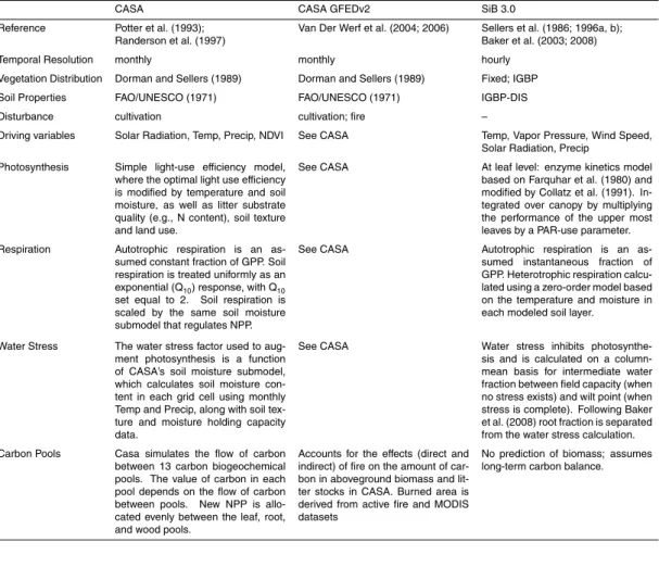
The three terrestrial biospheric models chosen for this analysis are the Simple Bio-sphere Model (SiB 3.0), the Carnegie Ames Stanford Approach (CASA) model, and CASA coupled with the Global Fire Emissions Database (CASA GFEDv2) (Table 1).

15

These models are used to evaluate the information that can be gained by applying the proposed methods. The models chosen as examples in this study differ in how they represent the processes controlling carbon exchange between the land and atmo-sphere, and were selected because (1) they have been widely applied across a variety of regions and (2) are frequently used as prior estimates in inverse modeling studies

20

(e.g., Gurney et al., 2004; Peters et al., 2007; Wang et al., 2007). There is growing awareness of the strong influence of prior estimates in inversion results (R ¨odenbeck et al., 2003; Michalak et al., 2004; Mueller et al., 2008). Therefore, understanding how forward model estimates of NEE, GPP, and R_Evary spatially and what drives this vari-ability is of great importance, not only for forward model intercomparisons, but also for

25

atmospheric inversion studies.

(8)

BGD

7, 7903–7943, 2010

Title Page

Tables Figures

◭ ◮

Back Close

Full Screen / Esc

Discussion

P

a

per

|

Dis

cussion

P

a

per

|

Discussion

P

a

per

|

Discussio

n

P

a

per

|

respiration and water availability are represented. Monthly NEE, GPP, and R_Eare com-pared among the models for 2002 over the domain of 10◦to 70◦N and 50◦to 170◦W, at a spatial resolution of 1◦×1◦ (approximately 110 km by 50 km; the distance per degree change in longitude varies across the domain).

2.1.1 Simple Biosphere Model (SiB 3.0)

5

SiB (Sellers et al., 1986, 1996a,b) is a biophysically-based, land-surface model in which the exchange of CO2 is linked to exchanges of water and heat at the vegetative

land-surface. Like other land-surface parameterizations, SiB 3.0 (Baker et al., 2008) is formulated based on the theory that the physiological controls operating at the plant level seek to maximize photosynthesis while minimizing water loss (Baker et al., 2003).

10

Thus, photosynthetic carbon fixation is based on enzyme kinetics (Farquhar et al., 1980), and linked to stomatal conductance through the Ball-Berry equation (Collatz et al., 1991). Soil respiration is calculated based on temperature and soil moisture in each soil layer. Overall, ecosystem respiration is forced within the model to balance annually with net uptake (Denning et al., 1996; Baker et al., 2003). SiB 3.0, hereafter

15

referred to as SiB, specifies spatial heterogeneity in some of its canopy properties through the use of satellite-derived vegetative indices such as leaf area index (LAI) and absorbed fraction of photosynthetically active radiation (PAR), rather than using published values of vegetation and soil parameters tied solely to vegetation type (Baker et al., 2003). SiB has been coupled with the Regional Atmospheric Modeling System

20

(e.g., SiB-RAMS) in regional inversion and error estimation studies (Denning et al., 2003; Nicholls et al., 2004; Zupanski et al., 2007; Lokupitiya et al., 2008).

2.1.2 Carnegie Ames Stanford Approach (CASA)

CASA is a biogeochemical model that uses a system of first-order linear differential equations to represent the flow of carbon between various pools, and track the

long-25

(9)

BGD

7, 7903–7943, 2010

Title Page

Tables Figures

◭ ◮

Back Close

Full Screen / Esc

Discussion

P

a

per

|

Dis

cussion

P

a

per

|

Discussion

P

a

per

|

Discussio

n

P

a

per

|

Randerson et al., 1997; Schaefer et al., 2008). CASA tracks photosynthesis using a simple light-use efficiency model, where maximum light-use efficiency is modified by factors such as temperature, water availability, and litter substrate quality. Heterotrophic (i.e., soil) respiration is simulated within a number of soil-organic carbon pools; whereas autotrophic respiration is assumed a constant fraction of GPP. The model’s soil

mois-5

ture submodel is used to regulate both plant production and respiration. This version of CASA is used asa prioriinformation in, among other studies, the TransCom3 inversion intercomparison study (e.g., Gurney et al., 2004; Baker et al. 2006). No component fluxes (e.g., GPP and RE) were available for this version of CASA.

2.1.3 CASA coupled with the Global Fire Emissions Database (CASA GFEDv2)

10

The CASA GFEDv2 model (van der Werf et al., 2004, 2006) is based on the CASA model described above, although fPAR is estimated from Advanced Very High Resolu-tion Radiometer (AVHRR) Normalized Difference Vegetation Index (NDVI) instead from NOAA/NASA Pathfinder NDVI (as in CASA). In addition, CASA GFEDv2 accounts for the indirect (e.g. mortality and subsequent decay and re-growth) effects of forest fires

15

on carbon stocks in CASA’s above-ground carbon pools (leaf, wood, and litter). In both CASA and CASA GFEDv2, the light utilization efficiency term is set uniformly to a value derived from calibration of predicted annual NPP to previous field estimates (Potter et al., 1993).

2.2 Spatial covariance of modeled fluxes

20

We apply variogram analysis to quantify monthly spatial autocorrelation of predicted NEE, and to examine how that variability changes with season. Here, autocorrelation is defined as the similarity of fluxes as a function of their separation distance, and is used as means to quantify spatial variability. This approach enables not only the estimation of spatial variability in each of the models, but, more importantly, the comparison of

25

(10)

BGD

7, 7903–7943, 2010

Title Page

Tables Figures

◭ ◮

Back Close

Full Screen / Esc

Discussion

P

a

per

|

Dis

cussion

P

a

per

|

Discussion

P

a

per

|

Discussio

n

P

a

per

|

NEE’s component fluxes (GPP and R_E) is quantified for the three summer months of June, July, and August.

Quantifying spatial autocorrelation is needed to inform the statistical analysis (e.g., Sect. 2.3), geared towards identifying potential drivers of observed spatial patterns of flux among the models. The comparison of spatial variability among the models also

5

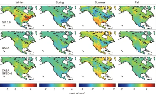
provides a quantitative counterpart to the visual examination of variability depicted in maps of the spatial pattern of fluxes (e.g., Fig. 1). Quantitative comparisons help to identify significant differences between the models, and can help to inform the compar-ison of model results.

A variogram is a function used to describe the spatial correlation of observations,

10

and is based on the degree of dissimilarity between two points,y(x) andy(x+h):

γ(h)=1 2E

h

(y(x+h)−y(x))2i (1)

Wherey represents the grid-scale flux (i.e., NEE, GPP, or R_E) predicted from the mod-els, andhis the separation distance between two grid-scale estimates of flux. The raw variogram derived from Eq. (1) is normally modeled using a theoretical variogram

func-15

tion. Here, we use an exponential model to examine the spatial correlation of a particu-lar biospheric model’s estimate of carbon flux. This choice is based on an examination of the raw variograms of flux estimates constructed from the different models, and is consistent with the work of Michalak et al. (2004). The exponential variogram is defined as:

20

γ(h)=σ2

1−exp

−h

l

(2)

whereσ2represents the expected variance of carbon flux at large separation distances, andl is the correlation range parameter. The practical correlation length (L) is approx-imately 3l, beyond which the covariance between points is negligible (e.g., Kitanidis, 1997).

(11)

BGD

7, 7903–7943, 2010

Title Page

Tables Figures

◭ ◮

Back Close

Full Screen / Esc

Discussion

P

a

per

|

Dis

cussion

P

a

per

|

Discussion

P

a

per

|

Discussio

n

P

a

per

|

To obtain an overall measure of spatial variability for each of the models, the spatial covariance parameters (σ2,l) of grid-scale estimates of flux for land cells within NA are optimized by fitting the theoretical variogram in Eq. (2) to the raw variogram (derived from Eq. (1) using ordinary least squares (OLS). Conceptually, a higher variance is indicative of greater overall spatial variability, while a shorter correlation length indicates

5

greater spatial variability at smaller scales.

In order to better compare the spatial variability in carbon flux predicted by the mod-els, the parameter h0 (Alkhaled et al., 2008) is used to merge information from the

fitted variance and correlation range parameters, and to provide an overall measure of spatial variability:

10

h0=−lln

1−γmax

σ2

(3)

wherel andσ2are the fitted variogram parameters for each model from Eq. (2), andh₀

represents the distance at which the variogram reaches a certain preset value (γmax).

Therefore, h0 provides a single diagnostic metric with which to compare the overall

spatial variability of the models. Both a higher regional variance (σ2) and a shorter

cor-15

relation range parameter (l) results in a shorter overallh0, indicating a greater degree

of spatial variability of the modeled flux over smaller spatial scales. The value of gmax used in the analysis of model estimates of NEE and component fluxes (GPP and R_E) was chosen to be 0.05 and 1.0 (µmol m−2s−1)2, respectively. The choice of this value is somewhat flexible, as long as it is below the lowest observedσ2.

20

2.3 Variable selection and regression analysis

The geostatistical regression (GR) approach presented here includes a combination of variable selection (e.g., Burnham and Anderson, 2002) and geostatistical regression (i.e. universal kriging) (e.g., Kitanidis, 1997) in order to identify the factors explain-ing the spatial variability in monthly predicted NEE, GPP, and RE among biospheric

25

(12)

BGD

7, 7903–7943, 2010

Title Page

Tables Figures

◭ ◮

Back Close

Full Screen / Esc

Discussion

P

a

per

|

Dis

cussion

P

a

per

|

Discussion

P

a

per

|

Discussio

n

P

a

per

|

variables, including model assumptions, the manner in which mechanistic processes are formulated within the model, and the chosen driver or input data. Variable selection methods provide a measure of the overall linear sensitivity of estimated fluxes to envi-ronmental variables, or other derived quantities such as Q10, without having to recreate

the complex relationships or formulations within the models. Even if these formulations

5

could be recreated, such an approach would be undesirable because it would not of-fer a common metric of comparison across models. Variable selection also provides a means to compare models in light of their differences (e.g., formulations, environ-mental drivers), and to evaluate whether the same environenviron-mental variables appear as significant in explaining the spatial variability in flux across models.

10

Similarly to multiple linear regression, the GR approach expresses the dependent variable, in this case the estimated NEE (or GPP or RE) predicted from the models,y,

as the sum of a deterministic component, (Xβ), and a stochastic term, (ε) (Kitanidis, 1997):

y₌Xβ₊ε (4)

15

The deterministic component represents the portion of the predicted flux that can be explained using a set of grid-scale environmental variables or covariates, while the stochastic component describes the spatial variability in flux that could not be explained by the deterministic component. The deterministic component takes the form ofXβ, were X is a (n×p) matrix containing columns of p environmental variables that are

20

scaled by a p×1 vector of unknown drift coefficients or weights (β). The simplest model is a spatially constant mean, where p=1, X is a vector of ones, and β is the constant mean. More complex models include both the constant mean and a linear combination of environmental variables that best describe or represent the physical process being modeled (e.g., Erickson et al., 2005; Gourdji et al., 2008; Mueller et al.,

25

(13)

BGD

7, 7903–7943, 2010

Title Page

Tables Figures

◭ ◮

Back Close

Full Screen / Esc

Discussion

P

a

per

|

Dis

cussion

P

a

per

|

Discussion

P

a

per

|

Discussio

n

P

a

per

|

The variable selection step provides a means of objectively selecting the environ-mental variables to be included in X, while the geostatistical regression is used to obtain the best estimate of the drift coefficients ( ˆβ) which represent the relationship of model-predicted NEE, GPP, and REto the selected environmental variables, along with

their associated uncertainties (σ_β2_ˆ).

5

Together, these two approaches have several advantages over previous model in-tercomparison approaches. First, the application of a variable selection method re-duces the risk of identifying spurious relationships between environmental variables and modeled fluxes as significant, because only variables that jointly provide signifi-cant explanatory power can be selected. Second, the combination of variable

selec-10

tion and regression analysis serves as a systematic sensitivity test of flux estimates to common environmental drivers used in biospheric models. Thus, biospheric models can be assessed by comparing which environmental variables are selected as part of the GR model (Sect. 2.3.1), and by comparing the estimated drift coefficients relating the selected environmental variables to each model’s estimate of flux (Sect. 2.3.2).

15

2.3.1 Bayes Information Criterion (BIC)

One of the most widely used variable or model selection techniques is the Bayes Infor-mation Criterion (BIC) (Schwarz, 1987). The BIC is typically favored over hypothesis testing approaches because it is able to objectively compare non-nested, competing models (Burnham and Anderson, 2002). The term “model” here refers toX, or a

collec-20

tion of environmental variables that, either individually or collectively, have the most ex-planatory power in terms of the spatial variability of biospheric-model-derived monthly NEE, GPP, and R_E.

Criterion-based approaches, such as the BIC, have been applied recently in stud-ies focused on model selection for geospatial data (Hoeting et al., 2006) and, more

25

(14)

BGD

7, 7903–7943, 2010

Title Page

Tables Figures

◭ ◮

Back Close

Full Screen / Esc

Discussion

P

a

per

|

Dis

cussion

P

a

per

|

Discussion

P

a

per

|

Discussio

n

P

a

per

|

is based on the idea that models should be compared based on their posterior prob-abilities (Schwarz, 1978). In other words, selecting the combination of environmental variables that is most probable (Forster, 2000) in terms of explaining the variability of fluxes, if we assume that at least one “model” is true.

The BIC criterion of a particular combination of environmental variables,Xj, with p

5

covariates andnobservations is given by (Schwarz, 1978):

BIC_j=−2lnLˆ_j+pln(n) (5)

where the likelihood, ˆLj, of a particular collection of environmental variables best

ex-plaining modeled flux, is a function of the unknown drift coefficients,β, and the covari-ance of the regression residuals,ε, assuming that the regression residuals (Sect. 2.3.2)

10

follow a Gaussian distribution (Mueller et al., 2010).

If the residuals are assumed second-order stationary (i.e., spatially constant mean; e.g., Xβ), and the correlation between two points is solely a function of separation distance, then the covariance of the regression residuals,ε, is

Q(h)=E[(y(x)−X β)(y(x+h)−X β)] (6)

15

Where y represents the grid-scale flux (i.e., NEE, GPP, or R_E) predicted by the bio-spheric model, Q(h) is the covariance of the residuals with a separation distance, h, and E[ ] denotes the expectation operator. Q is modeled using the exponential vari-ogram function presented in Eq. (1) (Sect. 2.2):

Q=σ2

exp

−h

l

(7)

20

(15)

BGD

7, 7903–7943, 2010

Title Page

Tables Figures

◭ ◮

Back Close

Full Screen / Esc

Discussion

P

a

per

|

Dis

cussion

P

a

per

|

Discussion

P

a

per

|

Discussio

n

P

a

per

|

regression (see Gourdji et al., 2008). Accounting for the fact that the drift coefficients βare unknown, the BIC equation becomes (Mueller et al., 2010):

BICj=ln|Q|+yT

Q−1−Q−1XXTQ−1X− 1

XTQ−1

y₊pln(n) (8)

The reader is referred to Burnham and Anderson (2002) for a more detailed description of BIC, and to Mueller et al. (2010) and Yadav et al. (2010) for additional information

5

on how the BIC approach has been applied in the context of NEE and component flux modeling.

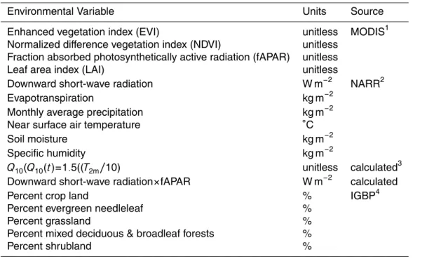
The BIC and GR analysis is conducted on 2002 monthly fluxes covering the three summer months of June, July and August. A small subset of monthly-averaged envi-ronmental variables is considered in the BIC analysis (Table 2). These variables were

10

chosen because they have full spatial coverage over North America and have a known association with biospheric fluxes. The variables in Table 2 were mean-deviated and normalized by their standard deviation prior to the regression analysis, in order to make estimated regression coefficients, ˆβ, comparable across variables.

2.3.2 Geostatistical regression analysis

15

Estimates of the drift coefficients, ˆβ, and the covariance matrix describing their uncer-tainties,V_βˆ, are obtained as (e.g., Cressie, 1993):

ˆ

β₌XTQ−1X−1XTQ−1y (9)

Vβˆ=

XTQ−1X−1 (10)

The diagonal elements of V_βˆ are the variances representing the uncertainty of the

20

(16)

BGD

7, 7903–7943, 2010

Title Page

Tables Figures

◭ ◮

Back Close

Full Screen / Esc

Discussion

P

a

per

|

Dis

cussion

P

a

per

|

Discussion

P

a

per

|

Discussio

n

P

a

per

|

quantified using the coefficient of determination:

R2=1−

y−XβˆTy−Xβˆ

(y−E[y])T(y−E[y]) (11)

WhereE[y] is the mean of the estimated flux from a given biospheric model.

3 Results and discussion

3.1 Spatial covariance

5

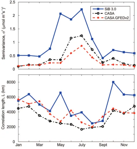
Non-growing season NEE consistently exhibits lower variances (σ2), reaching a mini-mum in October (∼0.2 to 0.5 (µmol m−2s−1)2), and remaining relatively constant until bud-burst and leaf-out in April and May (Fig. 2). The variance during the growing sea-son, on the other hand, is quite different between the models, with the greatest variance in NEE exhibited by SiB (Figs. 2 and 3). Similarly, correlation lengths (L) are generally

10

longer during the dormant months, which is consistent with the lower spatial variability observed in the variance parameter.

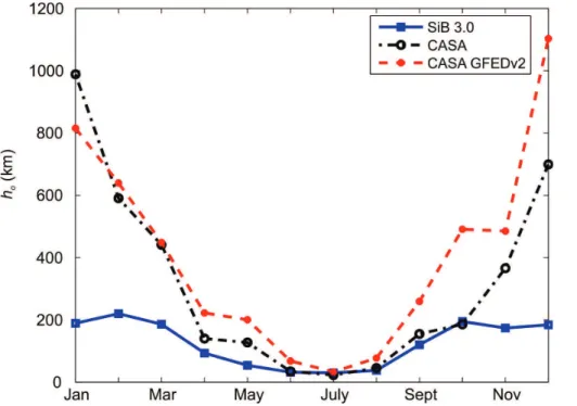
The h0 parameter (Eq. 3) confirms that NEE from SiB is more variable relative to

the other models for most months, and especially during the dormant months, followed by CASA and CASA GFEDv2 (Fig. 3). SiB’s forced cell-by-cell, long-term balance

15

in photosynthesis and respiration likely drives its greater spatial variability during the winter or dormant months, because the underlying spatial structure or variability is retained during the dormant season within SiB, much more so than for CASA or CASA GFEDv2.

Both SiB 3.0 and CASA GFEDv2’s predictions of GPP have significantly greater

spa-20

(17)

BGD

7, 7903–7943, 2010

Title Page

Tables Figures

◭ ◮

Back Close

Full Screen / Esc

Discussion

P

a

per

|

Dis

cussion

P

a

per

|

Discussion

P

a

per

|

Discussio

n

P

a

per

|

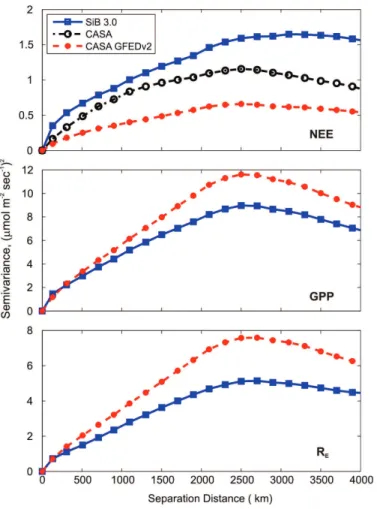
(see Fig. 4). The correlation lengths, however, of SiB’s summertime GPP and R_E (1100 km and 1300 km, respectively) are slightly shorter than for GFED (1200 km and 1400 km, respectively). Thus, using aγmaxof 1.0 (µmol m−

2

s−1)2, we see that the over-all spatial variability of GPP for SiB (h0=130 km) and CASA GFEDv2 (h0=110 km) are

comparable. However, CASA GFED (h0=190 km) exhibits slightly greater overall

spa-5

tial variability in RE during June, July, and August relative to SiB (h0=270 km). Recall

that the smallerh₀, the more variable the modeled flux over smaller spatial scales. The differing degrees of variability in REamong the models, combined with somewhat

com-parable degrees of variability in GPP, leads to the overall spatial variability observed in NEE. Conceptually, NEE is the small difference between two large fluxes: gross

10

primary productivity and ecosystem respiration. Large di_fferences in the variability of GPP and RE, as seen in SiB 3.0, can translate into more variability in resultant NEE

fluxes.

Both models assume autotrophic respiration to be a fraction of GPP; however, they compute heterotrophic respiration in different ways (Table 1). CASA GFEDv2 treats soil

15

respiration uniformly as a Q10 response. However, it scales respiration with the same

soil moisture submodel that regulates productivity (Table 1). Therefore, soil carbon flux is controlled by nondimensional scalars related to air temperature, soil moisture, litter substrate quality, and soil texture (Zhou et al., 2009). Conversely, SiB 3.0 calculates soil respiration from temperature and soil moisture in each layer, then scales respiration

20

to achieve carbon balance over an annual scale (Baker et al., 2003). No such annual balance is enforced in CASA GFEDv2, which allows carbon to accumulate and move through various carbon pools. In the summer months, this prescribed annual balance in SiB may dampen the soil respiration variability, and therefore ecosystem respiration, causing it to be less spatially variable (compared to CASA GFEDv2) at certain times of

25

the year.

(18)

BGD

7, 7903–7943, 2010

Title Page

Tables Figures

◭ ◮

Back Close

Full Screen / Esc

Discussion

P

a

per

|

Dis

cussion

P

a

per

|

Discussion

P

a

per

|

Discussio

n

P

a

per

|

also significantly impact how soil respiration is represented. Nevertheless, quantifying spatial variability allows for the comparison of flux estimates across models in terms of how differences in the degree of spatial variability in component fluxes translate into each model’s grid-scale estimates of NEE.

Overall, variogram analysis quantifies spatial variability among the models, which,

5

combined with knowledge about the model structure and formulations, is seen here to be a valuable tool for model intercomparisons. In addition, this type of information helps inform statistical analyses that correlate modeled fluxes to climatic variables and other environmental parameters. This is shown in the next section, where the spatial correlation structure described in Eq. (2) and shown in Fig. 2 is used to assess the

10

relationship of flux to environmental drivers and other ancillary variables.

3.2 Variable selection and regression analysis

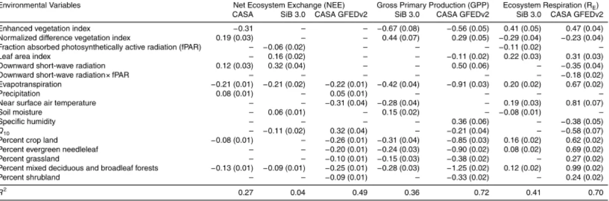
Drift coefficients and their associated uncertainties were estimated for those variables selected using the BIC as outlined in Sects. 2.3.1 and 2.3.2 (Table 3). A positive sign on ˆβi indicates the variable is associated with an increase in REor a decrease in GPP,

15

while a negative sign indicates that a variable is correlated with a net increase in GPP or decrease in RE.

3.2.1 Explanatory variables for modeled net ecosystem exchange

Only evapotranspiration and the percent land cover by mixed and deciduous forests (MDBF) were found to have a significant relationship with estimated NEE across all

20

models (Table 3). This is consistent with the expected strong relationship between tran-spiration and photosynthesis. The connection between land cover types, such as de-ciduous forest, and NEE is intuitive as well. Highly productive regions tend to have large gross fluxes, and small changes in these fluxes (relative to mean uptake/respiration) can have a large impact on net flux. Thus, the BIC successfully identifies variables with

25

(19)

BGD

7, 7903–7943, 2010

Title Page

Tables Figures

◭ ◮

Back Close

Full Screen / Esc

Discussion

P

a

per

|

Dis

cussion

P

a

per

|

Discussion

P

a

per

|

Discussio

n

P

a

per

|

The magnitude and sign of the drift coefficient ( ˆβ) for evapotranspiration in rela-tion to NEE is consistent among the three biospheric models (Table 3) indicating that evapotranspiration has a similar importance in each of the models or at least the spa-tial distribution of evapotranspiration is correlated similarly to the spaspa-tial distribution of NEE. In contrast, even though the percent cover of MDBF was selected as a significant

5

variable explaining NEE across models, its weight (i.e., drift coe_fficient) varies, with the greatest correlation observed for CASA GFEDv2 and the lowest correlation in SiB 3.0. The sign on the drift coefficients are consistent, however, with MDBF being associated with an overall uptake of CO₂across models (Table 3).

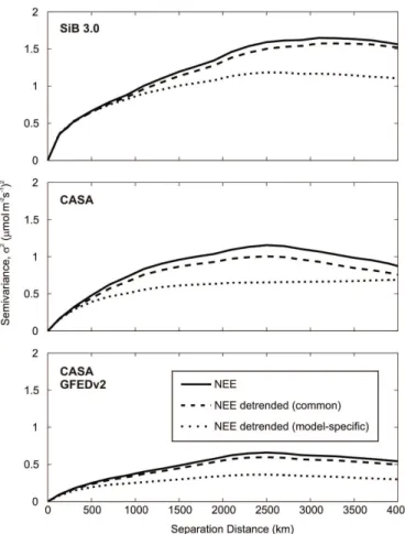
The amount of NEE’s spatial variability explained by the selected environmental

10

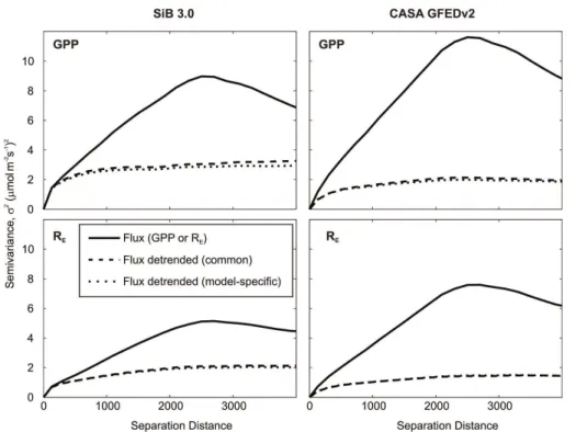
variables for each model is shown in Fig. 5 using experimental variograms (e.g., a smoothed variogram generated by averaging the raw variogram over consecutive separation distance intervals, similarly as for a histogram). Included in Fig. 5 is the ex-perimental variogram resulting if only those variables commonly selected across mod-els (i.e., evapotranspiration and MDBF) are used in the trend, as well as when each

15

model is detrended using all of the variables selected for that model (Xβˆ). Evapotran-spiration and percent cover of MDBF explain only a small portion of spatial variability in estimated NEE, compared to the complete model-specific environmental variables selected through BIC. This implies that the model-specific variables selected for each model are more important for interpreting the predicted carbon flux than are the

vari-20

ables commonly selected for all models. Such a finding is important because it sug-gests fundamental differences in the models and the factors that control predicted flux. For a given scale and time period, this in turn, provides an opportunity for comparing the variables selected for each model with those found to be important in explaining real flux observations (e.g., Law et al., 2002; Urbanski, 2008; Mueller et al., 2010;

Ya-25

(20)

BGD

7, 7903–7943, 2010

Title Page

Tables Figures

◭ ◮

Back Close

Full Screen / Esc

Discussion

P

a

per

|

Dis

cussion

P

a

per

|

Discussion

P

a

per

|

Discussio

n

P

a

per

|

In the analysis conducted with SiB fluxes, the GR approach selected the fraction of photosynthetically active radiation (fPAR), LAI, downward short-wave radiation, soil moisture, and Q10, in addition to evapotranspiration and percent cover by MDBF, as

having the greatest explanatory power for modeled NEE (Table 3). This is in contrast to those additional variables selected as having a significant relationship to CASA’s

5

NEE fluxes, which include the enhanced vegetation index (EVI), normalized difference vegetation index (NDVI), precipitation, and the percent land cover by croplands. While precipitation and percent cover by cropland were also selected for CASA GFEDv2, temperature, Q10, and land cover type appear to be more highly correlated with

mod-eled NEE than in the other two models. Some of the differences in variables selected

10

for a given model may be less important (e.g., LAI and fPAR, versus EVI and NDVI) because these variables are similar. What is interesting is that very few variables were commonly selected in CASA and CASA GFEDv2, even though the same base model is used for each (Table 3). In the modifications of CASA to account for fire, the mortality of woody vegetation in CASA GFEDv2 is scaled with the amount of tree cover.

There-15

fore, a cell with high percentage tree cover will have higher mortality than, for example, an open grassland. (van der Werf et al., 2003). Mortality rates due to fire have an indi-rect effect on respiration and productivity, and thus, might explain the higher apparent correlation of CASA GFEDv2 fluxes to percent land cover relative to CASA or SiB3.0.

Q₁₀ was selected for both SiB 3.0 and CASA GFEDv2 as having a significant

rela-20

tionship to NEE. However, in SiB, Q10 is correlated with uptake or sink in CO2 in SiB,

while in CASA GFEDv2 it is linked to an overall release (Table 3). For CASA GFEDv2, the drift coe_fficients of Q₁₀and evapotranspiration are highly correlated, and therefore their impact cannot be assessed independently. In examining the net apparent impact (Xβˆ) of temperature on NEE in CASA GFEDv2 (not shown), temperature accounts for

25

the greatest net uptake of CO₂, more than twice the magnitude of any other variable. Conversely, in SiB, evapotranspiration and Q10 are correlated with the greatest overall

uptake and downward shortwave radiation with the largest release of CO2 from the

(21)

BGD

7, 7903–7943, 2010

Title Page

Tables Figures

◭ ◮

Back Close

Full Screen / Esc

Discussion

P

a

per

|

Dis

cussion

P

a

per

|

Discussion

P

a

per

|

Discussio

n

P

a

per

|

To further examine these relationships and to compare the models, a similar analysis was conducted on NEE’s component fluxes of GPP and R_E. Because environmental variables, such as light, water availability, and temperature may have complex relation-ships with each other, as well as photosynthesis and respiration, isolating the GPP and R_E estimates from the models may allow for a more robust comparison of modeled

5

output.

3.2.2 Explanatory variables for modeled gross primary production

and respiration

In general, a greater number of environmental variables are consistently identified as being correlated with GPP and REacross models, than were observed in the analysis

10

conducted with NEE. In addition, for a given biospheric model, many of the same envi-ronmental variables are correlated to both GPP and R_E (Table 3). However, with most variables, the sign of the recovered drift coefficients on GPP and RE is reversed. In

the analysis of component fluxes, uptake of CO2(i.e., GPP) is denoted with a negative

sign, while a positive sign represents release of CO₂from the land to the atmosphere

15

(i.e., RE). Those environmental variables that are correlated with an uptake of CO2

from the atmosphere in the analysis with GPP, are correlated with a source of CO2

when examined against R_E. In CASA, CASA GFEDv2, and SiB 3.0, autotrophic respi-ration is formulated as being an instantaneous fraction of GPP. Therefore, the similar but opposite relationship of selected environmental variables to GPP and RE may be

20

a result of model formulation rather than a real association with the physiological pro-cesses driving RE. However, the heterotrophic contribution to RE could be 50% or

more, and the controls on heterotrophic respiration (RH) may vary among the models.

For example, in a study by Mueller et al. (2010), which examined the relationship of environmental variables to measured flux from an eddy-covariance flux tower, different

25

variables were found to be correlated with GPP than to RE. Thus, the degree to which

(22)

BGD

7, 7903–7943, 2010

Title Page

Tables Figures

◭ ◮

Back Close

Full Screen / Esc

Discussion

P

a

per

|

Dis

cussion

P

a

per

|

Discussion

P

a

per

|

Discussio

n

P

a

per

|

influence cancels out when the GR approach is used directly with model estimates of NEE. This can be seen in Table 3 when the results of the NEE analysis are compared to those of the component fluxes.

From the component flux analysis, it appears that temperature has a stronger cor-relation to RE in CASA GFEDv2 compared to SiB, which is the reverse of what was

5

observed in the NEE analysis, where temperature was correlated with a net uptake of CO₂(Table 3). Temperature was not selected in the GPP analysis with CASA GFEDv2. In terms of NEE, temperature may be acting as a proxy for another variable not included in the analysis, or the interaction of variables whose spatial coverage can be captured (in part) by temperature.

10

Vegetative indices appear to be similarly correlated to GPP and R_Ein SiB and CASA GFEDv2. While land cover classification appears to have a significant impact in both models, as also seen with NEE, the relationship to flux is stronger in CASA GFEDv2. The incremental impact of land cover is largest for deciduous and mixed broadleaf forests, evergreen and needleleaf forests, and croplands. This relationship between

15

flux and land cover makes intuitive sense. In areas where CO2 uptake is large (e.g.,

deciduous and mixed forests or croplands), respiration will likely be large as well. Fur-thermore, in regions where there are large gross fluxes, there is also the possibility for the largest variability in flux. The converse would be true for relatively unproductive regions, such as shrublands. This, combined with the potential impact of how mortality

20

rates are parameterized in CASA GFEDv2, explains the apparent strong relationship between percent land cover and CASA GFEDv2’s prediction of GPP, RE, and

subse-quently NEE.

The linear combination of selected variables (i.e., Xβˆ) associated with carbon up-take (GPP) and release (RE) explains approximately 70% of CASA GFEDv2 flux

vari-25

ability during the summer months and approximately half that amount for SiB 3.0 (Ta-ble 3). This can also be seen in Fig. 6, where the variability at smaller scales is only marginally reduced for SiB when GPP and RE are detrended using the selected

(23)

BGD

7, 7903–7943, 2010

Title Page

Tables Figures

◭ ◮

Back Close

Full Screen / Esc

Discussion

P

a

per

|

Dis

cussion

P

a

per

|

Discussion

P

a

per

|

Discussio

n

P

a

per

|

In addition, a significant proportion of the variability explained in both SiB and CASA GFED’s GPP and RE by their model-specific GR trends is from those variables

com-monly selected across both models (Fig. 6). The magnitude of the drift coefficients on these common variables differs between the two biospheric models, however, with larger drift coefficients estimated for CASA GFEDv2 fluxes versus SiB 3.0.

5

The greater overall ability of the GR models to explain component flux spatial vari-ability (and NEE) in CASA GFEDv2, compared to SiB, likely results for the types of candidate environmental variables used in this study (Table 2). CASA is a diagnostic model that uses remote sensing data as input. Thus, it makes sense that the flux es-timates from CASA would be more sensitive to datasets derived from remote sensing

10

information (e.g., vegetative indices, land cover). While SiB fluxes are also sensitive to similar ancillary environmental variables, these parameters explain far less of SiB’s spatial variability. Such a finding has several possible implications. If the true flux vari-ability does not significantly correlate with remote-sensing-based products, model esti-mates that strongly correlate with, and depend on, such datasets (such as those from

15

CASA) could potentially have significant biases. Conversely, more complex models, such as SiB, that derive their own measures of plant phenology based on environmen-tal conditions, depend heavily on their model formulation rather than the variability in observed environmental drivers. Self-derived quantities within such models could also introduce a bias if the process parameterizations do not emulate the behavior of the

20

(24)

BGD

7, 7903–7943, 2010

Title Page

Tables Figures

◭ ◮

Back Close

Full Screen / Esc

Discussion

P

a

per

|

Dis

cussion

P

a

per

|

Discussion

P

a

per

|

Discussio

n

P

a

per

|

4 Conclusions

This study proposes a set of quantitative methods, including variogram analysis, vari-able selection, and geostatistical regression, for comparing biospheric model estimates of NEE and its component fluxes. Using a small subset of biospheric models, these methods are evaluated in terms of their ability to identify overall similarities and

dif-5

ferences in modeled fluxes, quantify and compare the scales of variability among the models, and determine the environmental factors explaining the observed variability in fluxes.

Both the variogram analysis and the relatedh₀parameter provide information about the degree of flux spatial variability in the di_fferent models, beyond what is evident from

10

visual examination and comparison of flux patterns. The results show that while SiB exhibits greater variability in NEE than both CASA and CASA GFEDv2, particularly during the dormant and transition months of the year, the overall small scale variability in SiB’s component fluxes is much less than that of CASA GFEDv2. Moreover, it is these differences in the amount of variability in SiB’s RE and GPP that drive the

over-15

all variability observed in NEE. In addition, as seen with GPP and R_E,h0 is a single

diagnostic that allows for the comparison of complex variability, where the influence of variance and correlation length are merged to provide a more informative, and com-parable, measure of flux variability over smaller scales. Finally, information about flux autocorrelation helps to inform the regression analysis used to correlate modeled NEE

20

to common climatic and environmental parameters.

The GR approach, which combines variable selection and geostatistical regression, provides a means to identify and compare the environmental variables that are most significant in explaining modeled flux spatial variability. The approach highlights those environmental variables that correlate to flux as predicted by each examined model,

25

(25)

BGD

7, 7903–7943, 2010

Title Page

Tables Figures

◭ ◮

Back Close

Full Screen / Esc

Discussion

P

a

per

|

Dis

cussion

P

a

per

|

Discussion

P

a

per

|

Discussio

n

P

a

per

|

flux observations (e.g., eddy-covariance flux tower measurements or inventory-based estimates). For example, in a study conducted by Mueller et al. (2010) examining the factors explaining temporal flux variability at the University of Michigan Biological Sta-tion eddy covariance site, different environmental variables were found to be correlated with GPP than to R_E. This is contrary to the results of this analysis, which found the

bio-5

spheric model estimates of GPP and REto be sensitive to similar sets of environmental

variables. This inconsistency between the sensitivity of modeled and observed fluxes indicates that, for the examined models, predictions of R_Eappear to reflect a scaling of GPP, rather than sensitivity to environmental variables that control respiration directly. Whether this type of relationship is reasonable requires further investigation with other

10

models and flux measurements, and provides a new avenue for model-data intercom-parisons.

Furthermore, the GR analysis can be used to draw inferences about how differences in model formulation translate into observed di_fferences in flux variability across mod-els. For example, CASA GFEDv2’s method of scaling mortality with percent tree cover

15

appears to strongly influence its flux distribution. As a result, the spatial variability of carbon exchange across North America in CASA GFEDv2 is strongly correlated to land cover. In addition, SiB’s model formulation appears to be far more important in ex-plaining the spatial variability of fluxes than environmental factors such as temperature, precipitation, or land cover.

20

While the methods presented here can point to key differences between models, they cannot tell which model is more correct. For example, the regression approach presented cannot identify exactly which processes within the models are formulated realistically versus those that are modeled incorrectly. However, using the types of quantitative model evaluation methods presented here, in conjunction with existing

sci-25

(26)

BGD

7, 7903–7943, 2010

Title Page

Tables Figures

◭ ◮

Back Close

Full Screen / Esc

Discussion

P

a

per

|

Dis

cussion

P

a

per

|

Discussion

P

a

per

|

Discussio

n

P

a

per

|

environmental drivers.

Statistical methods, such as the ones applied here, represent powerful tools for com-paring biospheric model estimates of flux. Care must be taken in implementing and in-terpreting results from statistical analyses, however, because results can be impacted by the environmental variables considered and the spatiotemporal scale of the

analy-5

sis (e.g., 1◦×1◦spatial and monthly temporal resolution). Therefore the analysis should be set up to ensure that key variables or derived parameters needed to explain mod-eled flux variability are included in the analysis. The effect of missing environmental variables could be aliased onto other variables, thereby acting as a proxy for the true correlation. In addition, the conclusions have to be interpreted at the scale at which

10

the analysis was performed, both in terms of the time period covered (e.g., summer months), as well as the native spatial resolution of the models.

Overall, the quantitative approach presented here provides a toolset for compar-ing existcompar-ing model estimates of carbon flux, a task that has historically been difficult unless standardized simulations and forcing data are prescribed. The results show

15

that both variogram analysis and GR help to improve our understanding of model dif-ferences caused by alternative model formulations, which can be used as a guide for model enhancement, as well as for reconciling difference in modeled estimates of land-atmosphere carbon exchange. As such, tools such as those presented here provide an opportunity to improve large-scale biospheric model intercomparison studies.

20

Acknowledgements. The authors gratefully acknowledge Wilfred Post and Ian Baker for impor-tant feedback on this manuscript. In addition, the authors would like to thank Ian Baker and James Randerson for providing their model estimates for this work. This work was supported by the National Aeronautics and Space Administration under grant NNX06AE84G “Constrain-ing North American Fluxes of Carbon Dioxide and Inferr“Constrain-ing Their Spatiotemporal Covariances

25

(27)

BGD

7, 7903–7943, 2010

Title Page

Tables Figures

◭ ◮

Back Close

Full Screen / Esc

Discussion

P

a

per

|

Dis

cussion

P

a

per

|

Discussion

P

a

per

|

Discussio

n

P

a

per

|

References

Alkhaled, A. A., Michalak, A. M., Kawa, S. R., Olsen, S. C., and Wang, J. W.: A global evaluation of the regional spatial variability of column integrated CO₂ distributions, J. Geophys. Res.-Atmos., 113, doi:10.1029/2007jd009693, 2008.

Baker, I., Denning, A. S., Hanan, N., Prihodko, L., Uliasz, M., Vidale, P. L., Davis, K., and

5

Bakwin, P.: Simulated and observed fluxes of sensible and latent heat and CO₂ at the WLEF-TV tower using SiB2.5, Glob. Change Biol., 9, 1262–1277, 2003.

Baker, I. T., Prihodko, L., Denning, A. S., Goulden, M., Miller, S., and da Rocha, H. R.: Sea-sonal drought stress in the Amazon: reconciling models and observations, J. Geophys. Res.-Biogeo., 113, G00b01, doi:10.1029/2007jg000644, 2008.

10

Baldocchi, D., Falge, E., Gu, L. H., Olson, R., Hollinger, D., Running, S., Anthoni, P., Bern-hofer, C., Davis, K., Evans, R., Fuentes, J., Goldstein, A., Katul, G., Law, B., Lee, X. H., Malhi, Y., Meyers, T., Munger, W., Oechel, W., Paw U, K. T., Pilegaard, K., Schmid, H. P., Valentini, R., Verma, S., Vesala, T., Wilson, K., and Wofsy, S.: Fluxnet: a new tool to study the temporal and spatial variability of ecosystem-scale carbon dioxide, water vapor, and

en-15

ergy flux densities, B. Am. Meteorol. Soc., 82, 2415–2434, 2001.

Bondeau, A., Kicklighter, D. W., Kaduk, J., and participants Potsdam, N. P. P. M. I.: Comparing global models of terrestrial net primary productivity (NPP): importance of vegetation structure on seasonal NPP estimates, Glob. Change Biol., 5, 35–45, 1999.

Burnham, K. P. and Anderson, D. R.: Model Selection and Multimodel Inference: A Practical

20

Information-Theoretical Approach, 2nd edn., Springer Science, New York, 2002.

Chapin, F. S., Woodwell, G. M., Randerson, J. T., Rastetter, E. B., Lovett, G. M., Baldoc-chi, D. D., Clark, D. A., Harmon, M. E., Schimel, D. S., Valentini, R., Wirth, C., Aber, J. D., Cole, J. J., Goulden, M. L., Harden, J. W., Heimann, M., Howarth, R. W., Matson, P. A., McGuire, A. D., Melillo, J. M., Mooney, H. A., Neff, J. C., Houghton, R. A., Pace, M. L.,

25

Ryan, M. G., Running, S. W., Sala, O. E., Schlesinger, W. H., and Schulze, E. D.: Rec-onciling carbon-cycle concepts, terminology, and methods, Ecosystems, 9, 1041–1050, doi:10.1007/s10021-005-0105-7, 2006.

Chiles, J. P. and Delfiner, P.: Geostatistics: Modeling Spatial Uncertainty, John Wiley and Sons, New York, 695 pp. 1999.

30