The impact of near-surface soil moisture assimilation at subseasonal, seasonal, and inter-annual time scales

(1)

HESSD

12, 7971–8004, 2015

Soil moisture assimilation time

scales

C. Draper and R. Reichle

Title Page

Abstract Introduction

Conclusions References

Tables Figures

◭ ◮

Back Close

Full Screen / Esc

Printer-friendly Version Interactive Discussion

Discussion

P

a

per

|

Discussion

P

a

per

|

Discussion

P

a

per

|

Discussion

P

a

per

|

Hydrol. Earth Syst. Sci. Discuss., 12, 7971–8004, 2015 www.hydrol-earth-syst-sci-discuss.net/12/7971/2015/ doi:10.5194/hessd-12-7971-2015

This discussion paper is/has been under review for the journal Hydrology and Earth System Sciences (HESS). Please refer to the corresponding final paper in HESS if available.

The impact of near-surface soil moisture

assimilation at subseasonal, seasonal,

and inter-annual time scales

C. Draper1,2and R. Reichle1

1

Global Modeling and Assimilation Office, NASA GSFC, Greenbelt, MD, USA

2

Universities Space Research Association, Columbia, MD, USA

Received: 9 July 2015 – Accepted: 24 July 2015 – Published: 17 August 2015

Correspondence to: C. Draper (clara.draper@nasa.gov)

(2)

HESSD

12, 7971–8004, 2015

scales

Title Page

Tables Figures

◭ ◮

Back Close

Full Screen / Esc

Discussion

P

a

per

|

Discussion

P

a

per

|

Discussion

P

a

per

|

Discussion

P

a

per

|

Abstract

Nine years of Advanced Microwave Scanning Radiometer – Earth Observing System (AMSR-E) soil moisture retrievals are assimilated into the Catchment land surface model at four locations in the US. The assimilation is evaluated using the unbiased Mean Square Error (ubMSE) relative to watershed-scale in situ observations, with the

5

ubMSE separated into contributions from the subseasonal (SMshort), mean seasonal (SM_seas) and inter-annual (SM_long) soil moisture dynamics. For near-surface soil mois-ture, the average ubMSE for Catchment without assimilation was (1.8×10−3m3m−3)2, of which 19 % was in SM_long, 26 % in SM_seas, and 55 % in SM_short. The AMSR-E assim-ilation significantly reduced the total ubMSE at every site, with an average reduction of

10

33 %. Of this ubMSE reduction, 37 % occurred in SMlong, 24 % in SMseas, and 38 % in SM_short. For root-zone soil moisture, in situ observations were available at one site only, and the near-surface and root-zone results were very similar at this site. These results suggest that, in addition to the well-reported improvements in SMshort, assimilating a su_fficiently long soil moisture data record can also improve the model representation

15

of important long term events, such as droughts. The improved agreement between the modeled and in situ SMseas is harder to interpret, given that mean seasonal cycle errors are systematic, and systematic errors are not typically targeted by (bias-blind) data assimilation. Finally, the use of one year subsets of the AMSR-E and Catchment soil moisture for estimating the observation-bias correction (rescaling) parameters is

20

(3)

HESSD

12, 7971–8004, 2015

scales

Title Page

Tables Figures

◭ ◮

Back Close

Full Screen / Esc

Discussion

P

a

per

|

Discussion

P

a

per

|

Discussion

P

a

per

|

Discussion

P

a

per

|

1 Introduction

Remotely sensed near-surface soil moisture observations are typically assimilated us-ing a bias-blind assimilation of observations that have been “bias-corrected” to have the same mean as the model forecast soil moisture (Reichle et al., 2007; Scipal et al., 2008; Bolten et al., 2010). This approach is designed to avoid forcing the model into

5

a regime that is incompatible with its assumed (likely erroneous) structure and param-eters, or inadvertently introducing any observation biases into the model, while still allowing the assimilation to correct for random errors in the model forecasts (Reichle and Koster, 2004). Here “random” errors are defined as errors that persist for less than the time scale used to – subjectively – define the bias. Observation-bias correction

10

of remotely sensed soil moisture is usually achieved by rescaling the observations to have the same mean and variance as model forecasts, for example by matching their Cumulative Distribution Functions (CDFs; Reichle and Koster, 2004). Traditionally, the observation rescaling (CDF-matching) parameters are estimated over the maximum available coincident observed and forecast data record (Reichle et al., 2007; Scipal

15

et al., 2008; Draper et al., 2012), so that the rescaled observations will retain a sig-nal of any observation-forecast differences that occurred at time scales shorter than the data record. For a multi-year data record assimilating these rescaled observations could then potentially update the model soil moisture with observed information at sub-seasonal, sub-seasonal, and inter-annual time scales.

20

The physical processes causing soil moisture errors at the above-mentioned sub-seasonal, sub-seasonal, and inter-annual time scales will be quite different. Most notably, in many locations seasonal scale variability is dominated by the mean seasonal cy-cle (the annually repeating variability), and any errors in the mean seasonal cycy-cle will be systematic (with causes such as incorrect separation of the soil and vegetation

25

(4)

HESSD

12, 7971–8004, 2015

scales

Title Page

Tables Figures

◭ ◮

Back Close

Full Screen / Esc

Discussion

P

a

per

|

Discussion

P

a

per

|

Discussion

P

a

per

|

Discussion

P

a

per

|

with transient atmospheric forcing events. For example, rapid time scale (daily) soil moisture dynamics are driven by factors such as individual precipitation events and changes in cloud cover, while longer time scale (seasonal-plus) dynamics are driven by changes in the atmospheric supply and demand for moisture (Entin et al., 2000). Soil moisture errors at subseasonal scales could then be caused by factors such as

5

atmospheric noise in remotely sensed data, or errors in the daily meteorology of the model atmospheric forcing, while inter-annual scale errors could be caused by factors such as drift in the remote sensor calibration, or incorrect representation of atmospheric drought conditions in the atmospheric forcing.

The systematic nature of errors in the mean seasonal cycle is problematic for data

10

assimilation. Theoretically, (bias-blind) data assimilation is not designed, nor optimized, to correct for systematic errors. More practically, if the systematic differences are not due to model errors (i.e., are caused by observation errors, including representativity errors), then assimilating such information can seriously degrade model performance. Consequently, due to concerns over the accuracy of the seasonal cycle in remotely

15

sensed soil moisture, Drusch et al. (2005) suggested that soil moisture observation-bias correction for data assimilation might be better designed so that the model soil moisture seasonal cycle is retained by the assimilation, as has been done in several more recent studies (Bolten et al., 2010; Yilmaz et al., 2015).

In addition to the systematic nature of seasonal errors, the time scale dependence

20

of soil moisture errors may also be more generally problematic for observation rescal-ing. Even within time scales less than one month, Su and Ryu (2015) showed that the multiplicative (di_fferences in standard deviation) and additive (di_fferences in mean) components of the systematic differences between modeled and remotely sensed soil moisture differ across time scales. They highlight that this lack of stationarity cannot

25

be adequately addressed by using bulk statistics to estimate observation rescaling pa-rameters.

(5)

HESSD

12, 7971–8004, 2015

scales

Title Page

Tables Figures

◭ ◮

Back Close

Full Screen / Esc

Discussion

P

a

per

|

Discussion

P

a

per

|

Discussion

P

a

per

|

Discussion

P

a

per

|

into separate time series representing soil moisture dynamics at subseasonal, mean seasonal, and inter-annual time scales. We have used this decomposition to examine the differences between remotely sensed and modeled soil moisture at each time scale, how these difference affect observation rescaling, and how assimilating the remotely sensed observations impacts the model soil moisture at each time scale. The

decom-5

position is achieved by fitting each soil moisture time series with harmonic functions specified to target the mean seasonal cycle (SMseas), and the subseasonal (SMshort) and inter-annual (SMlong) dynamics.

By fitting the appropriate harmonic functions to each time series, we can separate the total mean square error of each soil moisture time series into contributions from each

10

time scale. This is a much more targeted evaluation of soil moisture dynamics at the specific time scales that can then be linked to physical processes than is usually under-taken. Standard evaluation methods focus on bias-blind metrics, such as the correlation or unbiased Root Mean Square Error (ubRMSE, which is calculated after removing the long term mean di_fference (Entekhabi et al., 2010b)). Both of these are sensitive to soil

15

moisture time series variability at all time scales. While anomaly correlations (Ranom), are also used to exclude the seasonal cycle, this is not done consistently, and does not allow the total error to be broken into contributing time scales. Depending on how the anomalies are calculated, Ranom measures subseasonal scale errors (anomalies de-fined relative to a simple moving average, as in Dorigo et al., 2015), or a combination

20

of inter-annual and subseasonal scale errors (anomalies defined relative to the mean seasonal cycle over multiple years as in Draper et al., 2012).

In the second part of this study, we also explore the impact on the assimilation of using short time periods for observation bias correction. When first introducing CDF-matching to rescale remotely sensed soil moisture prior to assimilation, Reichle and

25

(6)

(AMSR-HESSD

12, 7971–8004, 2015

scales

Title Page

Tables Figures

◭ ◮

Back Close

Full Screen / Esc

Discussion

P

a

per

|

Discussion

P

a

per

|

Discussion

P

a

per

|

Discussion

P

a

per

|

E) data set, and also extend their investigation by providing a more statistically robust analysis of the impact of using single-year scaling parameters in the assimilation. This part of the study is motivated by the recent launch of the NASA’s Soil Moisture Active Passive (SMAP) mission (Entekhabi et al., 2010a), as it will address the consequences of using short records to rescaling the observations during the early phases of the

5

SMAP mission.

2 Data and methods

Nine years of surface soil moisture retrievals from AMSR-E X-band data (Owe et al., 2008) have been assimilated into the Catchment land surface model (Koster et al., 2000), at four locations in the US. The impact of the assimilation on the model skill

10

is measured by comparison to watershed-scale in situ soil moisture observations col-lected by the Agricultural Research Service (ARS) of the United States Department of Agriculture (Jackson et al., 2010). Each of these data sets is first described below (Sect. 2.1), followed by a discussion of the assimilation approach (Sect. 2.2) and the method used to decompose soil moisture time series into subseasonal, seasonal, and

15

inter-annual time scales (Sect. 2.3).

2.1 The soil moisture data sets

For over a decade the ARS has been collecting soil moisture observations, at least hourly, using dense networks of in situ sensors at four watershed scale sites in the US: Reynolds Creek (RC), Walnut Gulch (WG), Little Washita (LW), and Little River (LR).

20

See Table 1 for the locations of each site. These observations are averaged across each network to produce a coarse scale soil moisture observation with spatial support similar to typical remotely sensed and modeled soil moisture estimates. Observations are potentially made at every 5 cm from 5–60 cm depth, although the 5 cm layer typi-cally has a longer and more complete record than the deeper layers. In this study, the

(7)

HESSD

12, 7971–8004, 2015

scales

Title Page

Tables Figures

◭ ◮

Back Close

Full Screen / Esc

Discussion

P

a

per

|

Discussion

P

a

per

|

Discussion

P

a

per

|

Discussion

P

a

per

|

near-surface soil moisture from Catchment and AMSR-E was evaluated using the 5 cm ARS observations, while the root-zone soil moisture from Catchment was evaluated using the average of the 5–60 cm observations (including only times with data reported for all layers). The ARS root-zone soil moisture was used at Little River only, due to very low observation counts over the study period at the other sites. Given that we will

5

focus on evaluating variance, we have not supplemented the ARS observations with observations from single sensor networks, such as SCAN (Schaefer et al., 2007). Un-like the locally dense in situ measurements from the ARS networks, the variance (and mean) of observations from single sensors cannot be assumed representative of the coarse scale soil moisture from Catchment and AMSR-E.

10

Level 3 Land Parameter Retrieval (LPRM) X-band AMSR-E near-surface soil mois-ture retrievals at 0.25◦ resolution were obtained for the grid cells surrounding each site in Table 1. At X-band the observations relate to a surface layer depth slightly less than 1 cm. Only the descending (1:30 a.m. LT) overpass has been used to avoid possi-ble differences in the climatological statistics of day- and night-time observations. The

15

sites were explicitly selected by ARS to avoid possible radio frequency interference and proximity to permanent open water, and the AMSR-E soil moisture retrievals were screened to remove observations with X-band vegetation optical depth above 0.8.

NASA’s Catchment land surface model was run over the 9 km EASE grid cells surrounding each study site, using atmospheric forcing fields from Modern Era

20

Retrospective-Analysis for Research (MERRA; Rienecker et al., 2011) and recently improved soil parameters (De Lannoy et al., 2014). The model initial conditions were first spun-up from January 1993 to January 2002 using a single member without per-turbations. The ensemble (including perturbations) was then spun-up from January to October 2002 (see Sect. 2.2 for details of the ensemble). For both the model open loop

25

and data assimilation model output, the ensemble average near-surface (0–5 cm) and root zone (0–100 cm) soil moisture is then reported.

(8)

HESSD

12, 7971–8004, 2015

scales

Title Page

Tables Figures

◭ ◮

Back Close

Full Screen / Esc

Discussion

P

a

per

|

Discussion

P

a

per

|

Discussion

P

a

per

|

Discussion

P

a

per

|

series spanned the AMSR-E data record, rounded down to nine full years from Octo-ber 2002 to SeptemOcto-ber 2011, however the Little River root-zone soil moisture obser-vations are not available before January 2004, and were truncated to the seven years from October 2004 to September 2011. Also, there were just 21 ARS observations at Reynolds Creek in the last year of this period, and so the Reynolds Creek time

se-5

ries were truncated to the eight years from October 2002 to September 2010. The ARS and AMSR-E sensors can only measure liquid soil moisture, and all data have been screened out when the Catchment model indicates frozen near-surface condi-tions. Since the Reynolds Creek site is frozen for an extended period each winter, liquid soil moisture is not well defined there during winter, and the Reynolds Creek

10

time series have then been truncated to remove winter, defined from 1 December to 10 March (the period during which the Catchment surface is continuously frozen for at least three of the eight years of the Reynolds Creek record).

2.2 The assimilation experiments

The assimilation experiments were performed using a one-dimensional bias-blind

En-15

semble Kalman Filter, with the same set-up and ensemble generation as in Liu et al. (2011). We used CDF-matching (Reichle and Koster, 2004) to rescale the observations prior to each assimilation experiment. The details of the time period used to estimate the observation scaling parameters are given in Sect. 3, before presenting each set of results. The benefits of each assimilation experiment have then been compared to

20

that of the Catchment model open loop ensemble mean, in which the same ensemble generation parameters were used, and no observations were assimilated.

2.3 Decomposition of soil moisture time series

We wish to decompose each soil moisture (SM) time series into separate components representing soil moisture dynamics at the subseasonal (SM_short), seasonal (SM_seas),

25

(9)

HESSD

12, 7971–8004, 2015

scales

Title Page

Tables Figures

◭ ◮

Back Close

Full Screen / Esc

Discussion

P

a

per

|

Discussion

P

a

per

|

Discussion

P

a

per

|

Discussion

P

a

per

|

can be isolated by fitting a function made up of the sum of sinusoidal functions. For-mally, for some observed time series, y, the function, ˆy, is fit for some selection of integerski:

ˆ

y(t)=a0+ Σk=k₁,k₂,...aksin

2πkt

n

+bkcos

2πkt

n

, (1)

where t is the time step and n is the length of the time series. 2πk_n is the (angular)

5

frequency for a sinusoid completingkcycles overntime steps (i.e., that has frequency

k/nper time unit), and ˆy fork=ki is referred to as thekithharmonic.a0is the mean ofy. If the time series is sampled at regular intervals and has no missing data, the sinusoids for individual harmonics are orthogonal and independent of each other. This is the basis for the discrete Fourier transform, which exactly fits Eq. (1) toy using the

10

firstn/2 harmonics (i.e.,ki=1, 2, 3,. . .n/2). In this study, we use multiple linear least squares regression to fit Eq. (1) to the soil moisture time series for a sum of harmonic frequencies selected to isolate the variability at each target time scale, as described below.

We define SMseas by fitting Eq. (1) to the soil moisture time series for some combi-15

nation of the annual harmonic frequencies (i.e., fork/nan integer multiple of 1 yr−1). The frequencies higher than 1 yr−1moderate the shape of ˆy to account for differences in the shape of the seasonal cycle from the single sinusoid described by the first har-monic. Typically, only a few annual harmonics are necessary to fit the seasonal cycle of geophysical variables (Scharlemann et al., 2008; Vinnikov et al., 2008). Here we define

20

SMseas to be the sum of the first two harmonics, since fitting additional harmonics did not improve the ability to predict withheld data, following the method of Narapusetty et al. (2009). Note that since the same annual harmonics are repeated each year, we are restricting SMseasto represent only the mean seasonal cycle, and any inter-annual variability at seasonal time scales, such as anomalous vegetation growth in a given

25

(10)

HESSD

12, 7971–8004, 2015

scales

Title Page

Tables Figures

◭ ◮

Back Close

Full Screen / Esc

Discussion

P

a

per

|

Discussion

P

a

per

|

Discussion

P

a

per

|

Discussion

P

a

per

|

We define SM_longby fitting Eq. (1) to the soil moisture time series using the harmonic frequencies lower than 1 yr−1 that divide into the number of years in the data record (i.e., fork/n=1/m, 2/m, 3/m. . .(m−1)/m, wheremis the time series length in years). Finally, we define SMshort as the residual:

SMshort=SM− hSMi −SMlong−SMseas (2)

5

where hSMi is the temporal mean soil moisture. Note that, as defined here, SM_long, SMseas, and SMshort are all zero-mean, since the time series mean was assigned toa0 in Eq. (1). The coverage statistics for each data set in Table 2 highlight that the AMSR-E and ARS observed time series are incomplete. When applied to incomplete time series, the sinusoids fitted by Eq. (1) are no longer necessarily independent, hence the fitted

10

SMseas and SMlong may not be independent. We opted not to use gap-filling prior to fitting Eq. (1), to keep the method simple, and because gap-filling would directly affect the SMshort dynamics. In Sect. 3, before using the decomposed time series we check for signs of strong dependence between the fitted SMlong, SMseas, and SMshort, by test-ing whether the sum of the variances of the three time scale components differs from

15

the variance of the original soil moisture time series. We assume that if there is no dif-ference (or little difference) then any dependence between SMlong, SMseas, and SMshort has only a minimal impact on our results. Following initial investigation with this test, the number of observations used at each location is maximized by comparing only model (or assimilation) estimates to ARS in situ measurements, avoiding direct comparison

20

of the incomplete ARS and AMSR-E time series (which would require cross-screening for the availability of both). Finally, we do not use the harmonic fit to interpolate missing data, and instead screen out the fitted SMlongand SMseasat times when the original soil moisture was not available. Also, at Reynolds Creek, where the time series has been truncated to remove frozen winters, the length of the year used to fit the harmonics was

25

similarly truncated.

(11)

mov-HESSD

12, 7971–8004, 2015

scales

Title Page

Tables Figures

◭ ◮

Back Close

Full Screen / Esc

Discussion

P

a

per

|

Discussion

P

a

per

|

Discussion

P

a

per

|

Discussion

P

a

per

|

ing averages are often used for calculating anomaly correlations (Draper et al., 2012; Dorigo et al., 2015). The length of the averaging windows were chosen to give close agreement with the results of the harmonic decomposition described above. For the moving average decomposition, the inter-annual soil moisture time series, SMMA_long, is defined as the 181 day moving average, and the seasonal cycle, SMMA_seas, is defined

5

for each day of the year by averaging the data from all years that fall within a 45 day window surrounding that day-of-year. As with the harmonic approach, the subseasonal time series, SMMA_short, is calculated as the residual, analogous to Eq. (2). The same data processing and quality control as for the harmonic decomposition is used, plus the moving averages are only calculated when at least 60 % of the data within the

averag-10

ing window are available.

3 Results

Below, the original AMSR-E, Catchment, and ARS soil moisture time series are exam-ined (Sect. 3.1), before being split into SM_seas, SM_long, and SM_short (Sect. 3.2). The distribution of variance across the different time scales for each soil moisture estimate

15

is then compared (Sect. 3.3), before the observations are rescaled (Sect. 3.4), and the benefit of assimilating the AMSR-E data into Catchment is assessed at each time scale (Sect. 3.5). Finally, the consequences of using a relatively short record to rescale the AMSR-E data is examined (Sect. 3.6).

3.1 The ARS, AMSR-E, and catchment time series

20

Figure 1 shows the original time series at each site. In general, soil moisture from in situ, modeled, and remotely sensed estimates have systematic differences in their be-havior, due to representativity or structural differences between each estimate (Reichle et al., 2004). These systematic di_fferences are clear in Fig. 1. The most obvious dif-ference is that the mean and variance of each estimate differ (see also Table 2). Both

(12)

HESSD

12, 7971–8004, 2015

scales

Title Page

Tables Figures

◭ ◮

Back Close

Full Screen / Esc

Discussion

P

a

per

|

Discussion

P

a

per

|

Discussion

P

a

per

|

Discussion

P

a

per

|

AMSR-E and Catchment are consistently biased high compared to the ARS soil mois-ture. Bias values for the model range from 0.01 m3m−3for Little Washita to 0.09 m3m−3 for Little River, and bias values for the AMSR-E retrievals range from 0.07 m3m−3 for Reynolds Creek to 0.21 m3m−3 for Little River. Additionally, the standard deviation of AMSR-E is two to three times larger than the other two estimates. Figure 1

demon-5

strates that this is due to greater noise, and also a prominent seasonal cycle at Little Washita and Little River that is not evident in the other time series.

In addition to the systematic differences in their mean and standard deviation re-ported above, there are more subtle differences between the soil moisture dynamics described by each estimate. For example, for both the surface and root-zone soil

mois-10

ture, the ARS time series tend to show a sharper response to individual rain events than does Catchment, with (relatively) larger peaks followed by more rapid dry down after each event. At Walnut Gulch this is particularly obvious, with ARS rapidly drying to a well defined lower limit after each precipitation event, while Catchment has a lesser response to individual events, and a stronger seasonal signal.

15

3.2 Soil moisture time series at each time scale

Figure 2 shows an example of the time scale decomposition, for the Catchment surface soil moisture at Little River, for both the harmonic and moving average approaches. The time series described by each method are similar in terms of the magnitude and timing of their dynamics, except that the moving average inter-annual soil moisture

20

includes more high-frequency variability than does the harmonic version. Evaluation of soil moisture at specific time scales should ideally be based on time series separated into independent time scale components. For the harmonic method, independence between the time series at each time scale is not guaranteed since the original time series were not complete, while for the moving average method, independence is not

25

expected.

(13)

HESSD

12, 7971–8004, 2015

scales

Title Page

Tables Figures

◭ ◮

Back Close

Full Screen / Esc

Discussion

P

a

per

|

Discussion

P

a

per

|

Discussion

P

a

per

|

Discussion

P

a

per

|

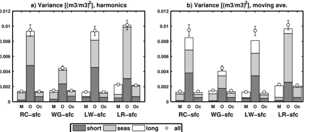
model and the AMSR-E observations. In Fig. 3a, for the harmonic method, the sum of the variances at each time scale (the stacked bars) is very close (within 2 %) to the total variance of the original soil moisture time series (the white circles), falling within the 95 % confidence interval of the total variance in each case. In contrast, for the moving average method in Fig. 3b the sum of the variances of each time scale

5

falls outside the 95 % confidence interval for the total time series variance at three of four sites, with a mean difference of 8 % of the total variance (with differences ranging between 1 and 16 %), indicating strong dependence between the three components. The sum of the variances of the time scale components is less than the total variance at each site, indicating positively correlated features between the moving average time

10

scale components (since h(σ_X2₊_Y)i=hσ_X2i −2hσX Yi+hσY2i). This positive correlation is

intuitively expected, since an anomaly in the original soil moisture time series has the same direction of influence on both the moving averages and the residual from that moving average (e.g., in Fig. 2 note the signal of the large positive anomaly in early 2004 in both SMMA_long and SMMA_short). Finally, the distribution of variance across the time

15

scales is similar for each method, largely because the moving average window lengths for SMMA_seas and SMMA_long were selected to generate time series closely matching those from the harmonic method.

3.3 Variance distribution across time scales

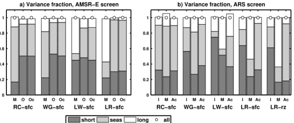
In Fig. 3 the AMSR-E variance is much larger than that for Catchment (as was

dis-20

cussed in Sect. 3.1), making it di_fficult to compare the relative distribution of variance across each time scale. Figure 4a then shows the AMSR-E and Catchment variance bar plots with the total variance normalized to one, to allow direct comparison to the fraction of variance at each time scale. The same plots are also presented for the Catchment and ARS soil moisture in Fig. 4b (recall we do not directly compare the

25

(14)

HESSD

12, 7971–8004, 2015

scales

Title Page

Tables Figures

◭ ◮

Back Close

Full Screen / Esc

Discussion

P

a

per

|

Discussion

P

a

per

|

Discussion

P

a

per

|

Discussion

P

a

per

|

noted from Fig. 1, AMSR-E has a very prominent seasonal cycle at Little River and Little Washita (40–70 % of the total variance) that is not present for Catchment or ARS, for which the SMseas fraction of variance is around 10–20 % in Fig. 4. In contrast, at Reynolds Creek and Walnut Gulch, Catchment has a larger fraction of its variance in the seasonal cycle (55–70 %) than does AMSR-E (20–40 %), with ARS agreeing with

5

Catchment at Reynolds Creek only. At Walnut Gulch the greater variance-fraction in the Catchment SM_seasis mostly balanced by less variability in SM_short(30 % compared to 60 % for ARS). This is associated with the differing responses to precipitation events already noted in Fig. 2.

AMSR-E could be expected a priori to have a larger fraction of variance at SM_short,

10

due to measurement noise in the remotely sensed observations. However, this is only the case at Reynolds Creek, where AMSR-E has 50 % of its variance in SMshort, com-pared to 20–30 % for Catchment and ARS. At Walnut Gulch, the AMSR-E and ARS SM_short variance-fractions are similar (50–60 %), while the fraction for Catchment is much lower (25 %). At Little Washita and Little River the variance-fraction in the

AMSR-15

E SMshort is similar to Catchment (at around 50 and 30 %, respectively) and both are much smaller than for ARS (around 70 %). At these two sites the AMSR-E SM_short variance-fraction may be less than expected due to the large amount of variance in its exaggerated seasonal cycle.

For the SM_long variance, the patterns at Little Washita and Little River are again

20

similar to each other. Catchment has much more variance in SMlong (40–50 %) than ARS (20 %) or AMSR-E (10 % or less). At the other two sites, the SMlong variance-fraction is similar for all data sets, except for the lower value for AMSR-E at Walnut Gulch (<10 %, compared to around 20 % for ARS and Catchment).

3.4 Baseline observation rescaling

25

(15)

HESSD

12, 7971–8004, 2015

scales

Title Page

Tables Figures

◭ ◮

Back Close

Full Screen / Esc

Discussion

P

a

per

|

Discussion

P

a

per

|

Discussion

P

a

per

|

Discussion

P

a

per

|

the model into a regime that is incompatible with its assumed structure and param-eters, leading to degraded flux forecasts (De Lannoy et al., 2007). For the baseline experiment, the AMSR-E observations were rescaled using bulk CDF-matching pa-rameters estimated over the full data record. By design, the CDF-matched AMSR-E observations, labeled Oc, have the same mean (not shown) and variance (Fig. 3a)

5

as the Catchment soil moisture. Figure 4 shows that the CDF-matching had little im-pact on the variance distributions across each time scale. This suggests that for the examples in this study, the CDF-matching operator could be approximated by a linear rescaling, in which only the mean and variance of the model are matched, as in Scipal et al. (2008). Hence, the observation rescaling, and assimilation of the resulting

obser-10

vations, was repeated using linear rescaling of the AMSR-E observations in place of CDF-matching, with very similar results in terms of the rescaled observations and the assimilation output (for both the Oc rescaling presented here, and the Oy rescaling in Sect. 3.6).

Recall that the distribution of the variance across di_fferent time scales was quite

15

different for AMSR-E and Catchment soil moisture in Fig. 4. Note that large errors in the variance at one time scale (in either AMSR-E or Catchment) will affect the rescaling of the variance at other time scales. In particular, if the unrealistically large AMSR-E seasonal cycle at Little Washita were replaced with something more realistic, for example representing 8 % of the total variance (as in the ARS time series), then the

20

fraction of variance in SM_short would increase from the current 48 to 75 %, increasing the SMshort variance in the CDF-matched AMSR-E from 0.0036 to 0.0054 (m

3 m−3)2.

3.5 Evaluation of the baseline assimilation experiment at each time scale

The improvement gained from assimilating the AMSR-E observations is evaluated us-ing the unbiased Mean Square Error (ubMSE) of the resultus-ing model soil moisture, with

25

(16)

HESSD

12, 7971–8004, 2015

scales

Title Page

Tables Figures

◭ ◮

Back Close

Full Screen / Esc

Discussion

P

a

per

|

Discussion

P

a

per

|

Discussion

P

a

per

|

Discussion

P

a

per

|

do not use the square root to take advantage of the additive property of the variance of independent time series, however to aid interpretation the ubMSE equivalent to the common ubRMSE target accuracy of 0.04 m3m−3is indicated in the relevant plots.

Figure 5 shows the ubMSE for each assimilation experiment, separated into each time scale. In the baseline assimilation experiment, labeled Ac, the observations

CDF-5

matched over the full time period (Oc) were assimilated into the Catchment model. Prior to assimilation, the average ubMSE in the near-surface soil moisture across the four sites was 1.8×10−3 (m3m−3)2 (giving a ubRMSE just above the 0.04 m3m−3target). Close to half (55 %) of the ubMSE is in SMshort, with the rest split between SMseas (26 %) and SM_long (19 %). The Ac assimilation significantly reduced the total ubMSE

10

at each site, reducing the average near-surface ubMSE across the four sites by 33 % to 1.2×10−3(m3m−3)2, with average reductions in the near-surface layer of 52 % for SMlong, 25 % for SMseas, and 22 % for SMshort. The total ubMSE was reduced at each site for all time scale components, except for SM_seasat Little Washita (where the model ubMSE was already relatively small).

15

Root-zone soil moisture observations were available for the study period only at Little River. Both the distribution of the ubMSE across each time scale, and the relative reductions achieved from assimilation, are similar for the near-surface and root-zone layers at Little River in Fig. 5d and e, adding confidence that the model improvements reported above for the near-surface soil moisture are indicative of the performance

20

throughout the soil profile.

To illustrate the impact of the assimilation at each time scale, Fig. 6 compares the decomposed time series for the Catchment model and Ac assimilation experiments to that from the ARS in situ observations at Little Washita. The difference between the three SMshort time series is difficult to visually judge in Fig. 6d, however, the impact 25

(17)

HESSD

12, 7971–8004, 2015

scales

Title Page

Tables Figures

◭ ◮

Back Close

Full Screen / Esc

Discussion

P

a

per

|

Discussion

P

a

per

|

Discussion

P

a

per

|

Discussion

P

a

per

|

amplitude, and also includes two maxima per year, where the ARS seasonal cycle has only one. The assimilation exacerbates the overestimated amplitude, but also removes the second annual maxima, resulting in an overall SMseasubMSE reduction (by 46 %).

3.6 Observation rescaling with a short data record

The nine year AMSR-E data record used here is the longest remotely sensed soil

5

moisture record available from a single satellite sensor, and soil moisture assimilation experiments using newer satellites are limited to shorter time periods. Obviously, as-similating a shorter time period will limit the potential improvements to the model SM_long (of similar magnitude to the SMshort improvement in this study). The potential benefit of an assimilation over a shorter period may also be limited by the increased sampling

10

uncertainty in the estimated observation rescaling parameters. This increased uncer-tainty could arise from systematic errors due to inadequate sampling of SMseas and SMlong, or from increased random errors associated with the smaller sample size. To establish the potential consequences of this uncertainty, we conducted nine additional experiments, labeled Ay, with the rescaling parameters for each estimated from a 12

15

month period starting in consecutive Octobers (but assimilating the full eight or nine year near-surface soil moisture data record listed in Table 1).

In contrast to Reichle and Koster (2004), we do not use ergodic substitution (of spa-tial sampling for temporal sampling) when estimating the rescaling parameters with a single year of observations, since with more modern remotely sensed data sets (than

20

the SMMR data used by Reichle and Koster, 2004) this is no longer necessary to ob-tain a sufficient sample size. Additionally, for the assimilation of Soil Moisture Ocean Salinity retrievals, De Lannoy and Reichle (2015) found ergodic substitution degraded the estimated CDFs, by introducing conflicting information from neighboring grid cells (possibly due to the higher spatial resolution, compared to SMMR).

25

(18)

HESSD

12, 7971–8004, 2015

scales

Title Page

Tables Figures

◭ ◮

Back Close

Full Screen / Esc

Discussion

P

a

per

|

Discussion

P

a

per

|

Discussion

P

a

per

|

Discussion

P

a

per

|

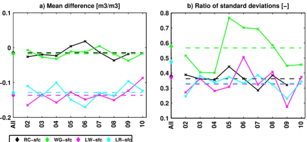
are addressed by the CDF-matching are the differences in the observed and forecast mean and standard deviation. For demonstrative purposes, Fig. 7 illustrates the diff er-ence between the means, and the ratio of the standard deviations, estimated using the full data record, and using each single year. In Fig. 7a there is considerable inter-annual scatter in the yearly mean differences, although by linearity the average is unbiased.

5

The standard deviation ratio in Fig. 7b also shows inter-annual variability, however the single year ratios are also biased low compared to the all-years ratio, since the single year estimates did not sample the SMlong variance (which was consistently a greater fraction of the total variance for Catchment than for AMSR-E in Fig. 4a). This is partic-ularly marked at Little River, where the average of the single year standard deviation

10

ratios was 30 % less than when estimated using all years (since SM_longmakes up close to 50 % of the total variance in Catchment, compared to less than 5 % for AMSR-E in Fig. 4a).

Figure 5 includes the ubMSE for the nine Ay assimilation experiments, as well as the mean ubMSE (hAyi) across all nine. Note that errors in the rescaling of the mean value

15

are likely under-reported here, since any introduction of biases into the model will not be directly detected by the ubMSE. Comparing the 35 individual Ay experiments to the baseline Ac experiments, most of the Ay experiments resulted in larger total ubMSE than the Ac experiment did at Reynolds Creek, Walnut Gulch, and Little Washita, while the opposite occurred at Little River. Overall there were eight Ay experiments for which

20

the total ubMSE was significantly different (at the 5 % level) and higher than for the Ac experiment, seven for which it was significantly different and lower, and 20 where the ubMSE was not significantly changed. The di_fferences between the Ac and Ay ubMSE are skewed, in that when the Ay ubMSE is higher, the difference tends to be greater than when it is lower. Consequently, the average reduction in the model ubMSE for the

25

near-surface soil moisture, compared to the model with no assimilation, is slightly less forhAyi(30 %) than for Ac (33 %).

(19)

HESSD

12, 7971–8004, 2015

scales

Title Page

Tables Figures

◭ ◮

Back Close

Full Screen / Esc

Discussion

P

a

per

|

Discussion

P

a

per

|

Discussion

P

a

per

|

Discussion

P

a

per

|

example, going through the experiments with the largest relative increase in ubMSE, experiment Ay07 at Reynolds Creek, and experiments Ay05, Ay06, and Ay07 at Walnut Gulch all have extreme standard deviation ratios, while Ay06 at Reynolds Creek and Ay10 at Little Washita have extreme mean differences. In each case, most of the in-crease in the ubMSE is due to inin-creased errors in the SMseasand SMlongcomponents, 5

suggesting that the SMshort corrections are more robust to uncertainty in the scaling parameters. The result that unrepresentative mean difference corrections can impact the ubMSE (a bias-robust metric) is interesting in that it demonstrates that bias-free assimilation of biased observations can degrade model soil moisture dynamics. Note also that unrepresentative scaling parameters do not necessarily degrade the

assimi-10

lation output, and in some instances are even advantageous. Most obviously, at Little River, where the single year standard deviation ratios were biased low (by 30 %), the Ay assimilation experiments all produced slightly lower ubMSE than the Ac experiment. Above, the assimilation of AMSR-E data that has been rescaled using parameters estimated from a single year, and from the full time period were compared, showing

15

that the average ubMSE is slightly higher when the single year parameters were used. However, it is perhaps more relevant to assess whether the assimilation is still benefi-cial when the single year parameters are used. Figure 5 suggests that on average it is. As with the Ac experiment, thehAyiubMSE is consistently less than that of the model at all time scales, except for SM_seasat Little Washita. However, for individual realizations

20

there is an increased risk when using the single year parameters that the assimilation will not significantly improve the model, or will even significantly degrade the model. For example, at Little Washita, where the Ac experiment reduced the ubMSE by a small but significant amount, none of the Ay experiments significantly decreased the ubMSE, and the Ay10 experiment significantly significantly increased it.

(20)

HESSD

12, 7971–8004, 2015

scales

Title Page

Tables Figures

◭ ◮

Back Close

Full Screen / Esc

Discussion

P

a

per

|

Discussion

P

a

per

|

Discussion

P

a

per

|

Discussion

P

a

per

|

4 Conclusions

Many studies have demonstrated that near-surface soil moisture assimilation can im-prove modeled soil moisture, in terms of the anomaly time series used to represent “random errors”, often implicitly assumed to represent subseasonal scale variability associated with individual precipitation events (Reichle et al., 2007; Scipal et al., 2008;

5

Draper et al., 2012). Here, nine-years of LPRM AMSR-E observations were assimi-lated into the Catchment model, and the resulting model output evaluated separately at the subseasonal (SMshort), seasonal (SMseas), and inter-annual (SMlong) time scales against watershed-scale in situ observations at four ARS sites in the US. The results show that, in addition to reducing the near-surface SM_short ubMSE averaged across

10

the four sites, the assimilation also reduced the near-surface SMlongubMSE. The mag-nitude of the reductions in SM_short and SM_long were similar (2.1×10−4(m3m−3)2, and 2.5×10−4(m3m−3)2, respectively), although this represented a much larger relative re-duction in the SMlongubMSE (52 % of the model SMlongubMSE, compared to 22 % for the SMshortubMSE). In situ observations of the root-zone layer were available for only 15

one site, however the similarity between the near-surface and root-zone results at this site (Fig. 5) is encouraging in terms our near-surface results being representative of the deeper soil moisture profile.

The reduced SM_longubMSE suggests that assimilating a sufficiently long data record of near surface soil moisture observations can improve the model soil moisture

dy-20

namics at inter-annual time scales, enhancing the model ability to simulate important events such as droughts. However, more so than for SM_short, it is possible that the re-duced ubMSE was associated with rere-duced representativity differences compared to the in situ observations that were used to calculate the ubMSE. For example, at Little River in Fig. 5 the substantial improvements to the SM_longnear-surface and root-zone

25

(21)

HESSD

12, 7971–8004, 2015

scales

Title Page

Tables Figures

◭ ◮

Back Close

Full Screen / Esc

Discussion

P

a

per

|

Discussion

P

a

per

|

Discussion

P

a

per

|

Discussion

P

a

per

|

that the model would benefit from correcting this error, in terms of improvements to forecast skill.

Assimilating the AMSR-E observations also reduced the near-surface SMseas ubMSE by 26 %, averaged across the four sites, suggesting the possibility that the assimilation was beneficial to the modeled mean seasonal cycle, despite not being

5

designed to address systematic errors. However, even more so than for SMlong, the re-duced SM_seasubMSE could be due to reduced representativity differences, rather than a genuine improvement to the model’s ability to represent the desired physical pro-cesses. To confirm that the SMlongand SMseasubMSE reductions do indicate improved model soil moisture would require evaluating the dependent moisture and energy flux

10

forecast, and unfortunately verifying observations are not available at the study loca-tions.

In comparing the AMSR-E and Catchment soil moisture at each time scale in this study, it became apparent that the distribution of variance across each time scale was very different between the remotely sensed and modeled soil moisture time series

15

(Fig. 4). Traditionally, observation rescaling strategies used in land data assimilation do not distinguish between variability at di_fferent time scales, and apply a single set of bulk rescaling parameters to the full time series. Consequently, the large discrepancies in the variance at one time scale (due to errors in one of or both estimates) can have follow-on e_ffects for the rescaling of other time scales. For example, the unrealistically

20

large AMSR-E seasonal cycle at Little Washita caused the variability at SMlong and SMshort to be overly dampened in this study. This could perhaps be avoided by using rescaling methods that rescale each time scale separately (e.g., Su and Ryu, 2015).

In addition to observation bias removal strategies that respect the time scale-dependent nature of observation – forecast systematic differences, it may be

advanta-25

(22)

HESSD

12, 7971–8004, 2015

scales

Title Page

Tables Figures

◭ ◮

Back Close

Full Screen / Esc

Discussion

P

a

per

|

Discussion

P

a

per

|

Discussion

P

a

per

|

Discussion

P

a

per

|

errors. This study is a first effort to investigate soil moisture assimilation at specific time scales associated with different soil moisture physical processes. Looking forward, fur-ther evaluation of soil moisture at these time scales will help to identify the physical processes responsible for errors in modeled and remotely sensed soil moisture (in-cluding representativity errors in the latter), which will in turn help to refine observation

5

bias removal strategies.

Finally, we have updated the investigation of Reichle and Koster (2004) into the use of short data records for estimating observation rescaling (CDF-matching) parameters. Nine additional assimilation experiments were performed, each with the AMSR-E ob-servations rescaled using parameters estimated from a single year of data. Compared

10

to the scaling parameters estimated using the full data record, using only one year of data introduced sampling errors due to inter-annual variability in SMseas and SMshort, and the unsampled SMlongvariability in the parameters.

For hindcasting/reanalysis applications, when the same short time period is used for bias parameter estimation and data assimilation, such unrepresentative parameters

15

should not be problematic, since the rescaled observations will still be unbiased rela-tive to the model over the length of the assimilation experiment, allowing shorter time scale errors to be corrected. However, in a forecasting/analysis application in which the bias corrections parameters must be estimated with the available (short) data record, and then applied to future observations, unrepresentative parameters can be more

20

problematic. Our results suggest that, when necessary, for example early in the SMAP mission, assimilating near-surface soil moisture over an extended period using single year parameters will introduce some additional uncertainty into the assimilation output, however over a large domain the overall impact will be minor. Of the total of 35 individ-ual assimilation realizations that we performed with single year parameters at the four

25

(23)

HESSD

12, 7971–8004, 2015

scales

Title Page

Tables Figures

◭ ◮

Back Close

Full Screen / Esc

Discussion

P

a

per

|

Discussion

P

a

per

|

Discussion

P

a

per

|

Discussion

P

a

per

|

the single year parameters was small, and did not practically reduce the benefit gained from the assimilation.

Acknowledgements. Thanks to Balachandrudu Narapusetty for helpful comments, USDA-ARS and Michael Cosh for providing access to the long term in situ soil moisture observations from the experimental watersheds. The AMSR-E soil moisture retrievals were obtained from the

5

NASA Goddard Earth Sciences Data and Information Services Center (GES DISC). This work was supported by the NASA Terrestrial Hydrology program (NNX15AB52G).

References

Bolten, J., Crow, W., Zhan, X., Jackson, T., and Reynolds, C.: Evaluating the utility of remotely-sensed soil moisture retrievals for operational agricultural drought monitoring, IEEE J. Sel.

10

Top. Appl., 3, 57–66, doi:10.1109/JSTARS.2009.2037163, 2010. 7973, 7974

De Lannoy, G. and Reichle, R.: Global assimilation of multi-angular SMOS brightness temper-ature observations into the GEOS-5 Catchment land surface model for soil moisture estima-tion, IEEE T. Geosci. Remote, submitted, 2015. 7987

De Lannoy, G., Reichle, R., Houser, P., Pauwels, V., and Verhoest, N.: Correcting for forecast

15

bias in soil moisture assimilation with the ensemble Kalman filter, Water Resour. Res., 43, W09410, doi:10.1029/2006WR005449, 2007. 7985

De Lannoy, G., Koster, R., Reichle, R., Mahanama, S., and Liu, Q.: An updated treatment of soil texture and associated hydraulic properties in a global land modeling system, J. Adv. Model. Earth Syst., 6, 957–979, doi:10.1002/2014MS000330, 2014. 7977

20

Dorigo, W., Gruber, A., de Jeu, R., Wagner, W., Stacke, T., Loew, A., Albergel, C., Brocca, L., Chung, D., Parinussa, R., and Kidd, R.: Evaluation of the ESA CCI soil mois-ture product using ground-based observations, Remote Sens. Environ., 162, 380–395, doi:10.1016/j.rse.2014.07.023, 2015. 7981

Draper, C., Reichle, R., De Lannoy, G., and Liu, Q.: Assimilation of passive

25

and active microwave soil moisture retrievals, Geophys. Res. Lett., 39, L04401, doi:10.1029/2011GL050655, 2012. 7973, 7981, 7990

Drusch, M., Wood, E., and Gao, H.: Observation operators for the direct assimilation of TRMM microwave imager retrieved soil moisture, Geophys. Res. Lett., 32, L15403, doi:10.1029/2005GL023623, 2005. 7974

(24)

HESSD

12, 7971–8004, 2015

scales

Title Page

Tables Figures

◭ ◮

Back Close

Full Screen / Esc

Discussion

P

a

per

|

Discussion

P

a

per

|

Discussion

P

a

per

|

Discussion

P

a

per

|

Entekhabi, D., Njoku, E., O’Neill, P., Kellogg, K., Crow, W., Edelstein, W., Entin, J., Good-man, S., Jackson, T., Johnson, J., Kimball, J., Piepmeier, J., Koster, R., Martin, N., McDon-ald, K., Moghaddam, M., Moran, S., Reichle, R., Shi, J., Spencer, M., Thurman, S., Tsang, L., and Van Zyl, J.: The Soil Moisture Active Passive (SMAP) mission, P. IEEE, 98, 704–716, doi:10.1109/jproc.2010.2043918, 2010a. 7976

5

Entekhabi, D., Reichle, R., Koster, R., and Crow, W.: Performance metrics for soil moisture retrievals and application requirements, J. Hydrometeorol., 11, 832–840, doi:10.1175/2010JHM1223.1, 2010b. 7975, 7985

Entin, J., Robock, A., Vinnikov, K., Hollinger, S., Liu, S., and Namkhai, A.: Temporal and spatial scales of observed soil moisture variations in the extratropics, J. Geophys. Res., 105, 11865–

10

11877, doi:10.1029/2000JD900051, 2000. 7974

Jackson, T., Cosh, M., Bindlish, R., Starks, P., Bosch, D., Seyfried, M., Goodrich, D., Moran, M., and Du, J.: Validation of advanced microwave scanning radiometer soil moisture products, IEEE T. Geosci. Remote, 48, 4256–4272, doi:10.1109/TGRS.2010.2051035, 2010.

Koster, R., Suarez, M., Ducharne, A., Stieglitz, M., and Kumar, P.: A catchment-based approach

15

to modeling land surface processes in a general circulation model: 1. Model structure, J. Geo-phys. Res., 105, 24809–24822, doi:10.1029/2000JD900327, 2000. 7976

Liu, Q., Reichle, R., Bindlish, R., Cosh, M., Crow, W., de Jeu, R., De Lannoy, G., Huffman, G., and Jackson, T.: The contributions of precipitation and soil moisture observations to the skill of soil moisture estimates in a land data assimilation system, J. Hydrometeorol., 12, 750–

20

765, doi:10.1175/JHM-D-10-05000.1, 2011. 7978

Narapusetty, B., DelSole, T., and Tippett, M.: Optimal estimation of the climatological mean, J. Climate, 22, 4845–4859, doi:10.1175/2009JCLI2944.1, 2009. 7979

Owe, M., de Jeu, R., and Holmes, T.: Multisensor historical climatology of satellite-derived global land surface moisture, J. Geophys. Res., 113, F01002, doi:10.1029/2007JF000769,

25

2008.

Reichle, R. and Koster, R.: Bias reduction in short records of satellite soil moisture, Geophys. Res. Lett., 31, L19501, doi:10.1029/2004GL020938, 2004. 7973, 7975, 7978, 7987, 7992 Reichle, R., Koster, R., Dong, J., and Berg, A.: Global soil moisture from satellite observations,

land surface models, and ground data: implications for data assimilation, J. Hydrometeorol.,

30

5, 430–442, doi:10.1175/1525-7541(2004)005<0430:GSMFSO>2.0.CO;2, 2004. 7981 Reichle, R., Koster, R., Liu, P., Mahanama, S., Njoku, E., and Owe, M.: Comparison and

(25)

HESSD

12, 7971–8004, 2015

scales

Title Page

Tables Figures

◭ ◮

Back Close

Full Screen / Esc

Discussion

P

a

per

|

Discussion

P

a

per

|

Discussion

P

a

per

|

Discussion

P

a

per

|

for the Earth Observing System (AMSR-E) and the Scanning Multichannel Microwave Ra-diometer (SMMR), J. Geophys. Res., 112, D09108, doi:10.1029/2006JD008033, 2007. 7973, 7990

Rienecker, M., Suarez, M., Gelaro, R.. Todling, R., Bacmeister, J., Liu, E., Bosilovich, M., Schu-bert, S., Takacs, L., Kim, G.-K., Bloom, S., Chen, J., Collins, D., Conaty, A., da Silva, A., Gu,

5

W., Joiner, J., Koster, R., Lucchesi, R., Molod, A., Owens, T., Pawson, S., Pegion, P., Red-der, C., Reichle, R., Robertson, F., Ruddick, A., Sienkiewicz, M., and Woollen, J.: MERRA – NASA’s Modern-Era Retrospective Analysis for Research and Applications, J. Climate, 24, 3624–3648, doi:10.1175/JCLI-D-11-00015.1, 2011.

Schaefer, G., Cosh, M., and Jackson, T.: The USDA Natural Resources Conservation

Ser-10

vice Soil Climate Analysis Network (SCAN), J. Atmos. Ocean. Tech., 24, 2073–2077, doi:10.1175/2007JTECHA930.1, 2007. 7977

Scharlemann, J., Benz, D., Hay, S., Purse, B., Tatem, A., Wint, G. W., and Rogers, D.: Global data for ecology and epidemiology: a novel algorithm for temporal fourier processing MODIS data, PLOS ONE, 1, e1408, doi:10.1371/journal.pone.0001408, 2008. 7979

15

Scipal, K., Drusch, M., and Wagner, W.: Assimilation of a ERS scatterometer derived soil mois-ture index in the ECMWF numerical weather prediction system, Adv Water Resour, 31, 1101– 1112, doi:10.1016/j.advwatres.2008.04.013, 2008. 7973, 7985, 7990

Su, C.-H. and Ryu, D.: Multi-scale analysis of bias correction of soil moisture, Hydrol. Earth Syst. Sci., 19, 17–31, doi:10.5194/hess-19-17-2015, 2015. 7974

20

Vinnikov, K., Yu, Y., Rama Varma Raja, M., Tarpley, D., and Goldberg, M.: Diurnal-seasonal and weather-related variations of land surface temperature observed from geostationary satel-lites, Geophys. Res. Lett., 35, L22708, doi:10.1029/2008gl035759, 2008. 7979

Yilmaz, M., Crow, W., and Ryu, D.: Impact of model relative accuracy in framework of rescaling observations in hydrological data assimilation studies, Water Resour. Res., submitted, 2015.

25

(26)

HESSD

12, 7971–8004, 2015

scales

Title Page

Tables Figures

◭ ◮

Back Close

Full Screen / Esc

Discussion

P

a

per

|

Discussion

P

a

per

|

Discussion

P

a

per

|

Discussion

P

a

per

|

Table 1.Location and time period of study sites.

Name (abbreviation) Location Time period

Reynolds Creek, surface (RC-sfc) 116.7◦W, 43.2◦N Oct 2002–Sep 2010, excluding 1 Dec–10 Mar Walnut Gulch, surface (WG-sfc) 110.0◦W, 31.7◦N Oct 2002–Sep 2011

(27)

HESSD

12, 7971–8004, 2015

scales

Title Page

Tables Figures

◭ ◮

Back Close

Full Screen / Esc

Discussion

P

a

per

|

Discussion

P

a

per

|

Discussion

P

a

per

|

Discussion

P

a

per

|

Table 2.Descriptive statistics for each data set at each study site.

Data source Number of data Mean (m3m−3) Standard deviation (m3m−3)

Reynolds Creek, surface

AMSR-E 1209 0.17 0.097

ARS 1944 0.10 0.068

Catchment 2111 0.16 0.039

Walnut Gulch, surface

AMSR-E 1960 0.15 0.067

ARS 3282 0.05 0.023

Catchment 3287 0.14 0.039

Little Washita, surface

AMSR-E 1748 0.27 0.097

ARS 2690 0.13 0.054

Catchment 3287 0.14 0.039

Little River, surface

AMSR-E 1989 0.31 0.100

ARS 3155 0.10 0.044

Catchment 3287 0.19 0.049

Little River, root-zone

AMSR-E – – –

ARS 2808 0.09 0.036

(28)

HESSD

12, 7971–8004, 2015

scales

Title Page

Tables Figures

◭ ◮

Back Close

Full Screen / Esc

Discussion

P

a

per

|

Discussion

P

a

per

|

Discussion

P

a

per

|

Discussion

P

a

per

|

0 0.2 0.4

a) RC−sfc: SM [m3/m3] ARS CATCH. AMSR−E

0 0.2 0.4

b) WG−sfc: SM [m3/m3]

0 0.2 0.4

c) LW−sfc: SM [m3/m3]

0 0.2 0.4

d) LR−sfc: SM [m3/m3]

2003 2004 2005 2006 2007 2008 2009 2010 2011

0 0.1 0.2

0.3e) LR−rz: SM [m3/m3]

(29)

HESSD

12, 7971–8004, 2015

scales

Title Page

Tables Figures

◭ ◮

Back Close

Full Screen / Esc

Discussion

P

a

per

|

Discussion

P

a

per

|

Discussion

P

a

per

|

Discussion

P

a

per

|

0 0.1 0.2 0.3 0.4

a) LR−sfc: SM (red points) & SM_long+SM_seas+<SM> (lines) HA MA

−0.2 −0.1 0 0.1 0.2

b) LR−sfc: SM_long

−0.2 −0.1 0 0.1 0.2

c) LR−sfc: SM_seas

2003 2004 2005 2006 2007 2008 2009 2010 2011

−0.2 −0.1 0 0.1 0.2

d) LR−sfc: SM_short

(30)

HESSD

12, 7971–8004, 2015

scales

Title Page

Tables Figures

◭ ◮

Back Close

Full Screen / Esc

Discussion

P

a

per

|

Discussion

P

a

per

|

Discussion

P

a

per

|

Discussion

P

a

per

|

M O Oc M O Oc M O Oc M O Oc

0 0.002 0.004 0.006 0.008 0.01 0.012

a) Variance [(m3/m3)2], harmonics

RC−sfc WG−sfc LW−sfc LR−sfc

M O Oc M O Oc M O Oc M O Oc

0 0.002 0.004 0.006 0.008 0.01 0.012

b) Variance [(m3/m3)2], moving ave.

RC−sfc WG−sfc LW−sfc LR−sfc

short seas long all