www.hydrol-earth-syst-sci.net/17/3895/2013/ doi:10.5194/hess-17-3895-2013
© Author(s) 2013. CC Attribution 3.0 License.
Hydrology and
Earth System
Sciences
Propagation of soil moisture memory to streamflow and
evapotranspiration in Europe
R. Orth and S. I. Seneviratne
Institute for Atmospheric and Climate Science, ETH Zurich, Universitätstrasse 16, 8092 Zurich, Switzerland
Correspondence to:R. Orth ([email protected]) and S. I. Seneviratne ([email protected])
Received: 10 October 2012 – Published in Hydrol. Earth Syst. Sci. Discuss.: 26 October 2012 Revised: 29 August 2013 – Accepted: 5 September 2013 – Published: 11 October 2013
Abstract.As a key variable of the land-climate system soil moisture is a main driver of streamflow and evapotranspi-ration under certain conditions. Soil moisture furthermore exhibits outstanding memory (persistence) characteristics. Many studies also report distinct low frequency variations for streamflow, which are likely related to soil moisture mem-ory. Using data from over 100 near-natural catchments lo-cated across Europe, we investigate in this study the con-nection between soil moisture memory and the respective memory of streamflow and evapotranspiration on different time scales. For this purpose we use a simple water bal-ance model in which dependencies of runoff (normalised by precipitation) and evapotranspiration (normalised by radia-tion) on soil moisture are fitted using streamflow observa-tions. The model therefore allows us to compute the mem-ory characteristics of soil moisture, streamflow and evapo-transpiration on the catchment scale. We find considerable memory in soil moisture and streamflow in many parts of the continent, and evapotranspiration also displays some mem-ory at monthly time scale in some catchments. We show that the memory of streamflow and evapotranspiration jointly de-pend on soil moisture memory and on the strength of the cou-pling of streamflow and evapotranspiration to soil moisture. Furthermore, we find that the coupling strengths of stream-flow and evapotranspiration to soil moisture depend on the shape of the fitted dependencies and on the variance of the meteorological forcing. To better interpret the magnitude of the respective memories across Europe, we finally provide a new perspective on hydrological memory by relating it to the mean duration required to recover from anomalies exceeding a certain threshold.
1 Introduction
Many past and recent publications have pointed out the remarkable persistence characteristics of soil moisture (Delworth and Manabe, 1988; Vinnikov and Yeserkepova, 1990; Entin et al., 2000; Koster and Suarez, 2001; Schlosser and Milly, 2002; Wu and Dickinson, 2004; Seneviratne et al., 2006; Koster et al., 2010; Seneviratne and Koster, 2012). This soil moisture persistence, hereafter referred to as “mem-ory”, is caused by the integrative nature of soil moisture as water storage. It has been found in observations and models, at point scale and on continental scales. Furthermore, also for other land-surface variables, persistence characteristics have been reported, even if less pronounced than for soil mois-ture. For instance streamflow exhibits distinct low frequency variations that represent a memory resulting from a recession behaviour of the streamflow response following a precipita-tion event (Rodriguez-Iturbe and Valdes, 1979; Lins, 1997; Labat, 2008; Gudmundsson et al., 2011).
Given the important role of soil moisture in the water cycle and for land-atmosphere interactions (e.g. Seneviratne et al., 2010, for a review), the question arises if its memory may propagate to other quantities that are at least partly driven by soil moisture. For example, runoff and evapotranspira-tion may be highly dependent on soil moisture under certain conditions (Eagleson, 1978; Koster and Milly, 1997; Koster et al., 2004; Botter et al., 2007; Bisselink and Dolman, 2009; Kirchner, 2009; Teuling et al., 2009), therefore soil moisture memory may induce persistence in these quantities.
prediction and water resource management. An evapotran-spiration memory has implications for the exchange of wa-ter between the land and the atmosphere, as well as for near-surface temperature because evapotranspiration is (neg-atively) related with sensible heat flux. Following the ap-proach proposed in Orth et al. (2013), we calibrate a sim-ple hydrological model (Koster and Mahanama, 2012) with streamflow measurements from 100 catchments across Eu-rope to infer memory characteristics of soil moisture, stream-flow and evapotranspiration. Note that soil moisture as in the formulation of this model represents a large fraction of the terrestrial water content that is altered by evapotranspira-tion, precipitation and surface runoff. We identify drivers and properties of the propagation of soil moisture memory and investigate their dependencies on regional features. More-over, we determine favourable climate and land-atmosphere regimes that promote memory propagation into the climate system. In the last part of this study, we investigate how the memories in soil moisture, streamflow and evapotranspira-tion change under dry and wet condievapotranspira-tions, which is especially relevant for the predictability of extreme events (Koster et al., 2010; Mueller and Seneviratne, 2012).
2 Methodology
2.1 Simple water-balance model
We use a simple water-balance model adapted from Koster and Mahanama (2012) in this study. The revised formulation employed here has been introduced and discussed in Orth et al. (2013). As in that study, we run the model with a daily time step. The model is based on the following water-balance equation:
Sn+△t=Sn+(Pn−En−Qn)△t (1)
whereSn, the only prognostic variable of the model (in mm),
is the total terrestrial water content at the beginning of time stepn. Between time stepnandn+ △t, the water content is
changed by the accumulated precipitationPn,
evapotranspi-rationEn, and streamflowQn(all in mm d−1), to yield an
up-dated terrestrial water contentSn+△t at the beginning of the
following time step. The employed simple model is highly conceptual, and thatSnis composed of (i) an upper level
stor-age, which represents the total soil moisture content,wn, and
(ii) a lower level storage, which represents groundwater,gn.
Note that as the model is simple and conceptual, this distinc-tion is an approximadistinc-tion. Precipitadistinc-tion is distributed to both storages and to streamflow. Note that snow is not considered in the simple water balance model. As in Orth et al. (2013), we run the model in this study with a time step of one day (△t=1d).
2.1.1 Evapotranspiration
In the simple water-balance model, evapotranspiration (nor-malised by net radiation) depends on soil moisture (scaled with the water holding capacity) only:
λρwEn
Rn
=β0
w
n
cs
γ
withγ >0 and β0≤1 (2)
whereRn denotes net radiation (in W m−2),λis the latent
heat of vaporization (in J kg−1),ρ
w is the density of water
(in kg m−3) andc
s is a model parameter that refers to the
water holding capacity of the soil (in mm). Another model parameter,β0(unitless), allows to capture the evaporative
re-sistance of the soil and the vegetation, whereas the parameter
γ (also unitless) ensures a strictly monotonically increasing
evapotranspiration ratioλρwEn
Rn
.
2.1.2 Streamflow and runoff
We distinguish in the simple water balance model between streamflowQn and runoff Run (note that this notation
dif-fers from Orth et al., 2013, whereS ist used for streamflow
andQdenotes runoff). As already suggested by Wood et al.
(1992), only a fraction of the precipitation can be stored in the soil, the remainder constitutes the runoff Run; and this
partitioning depends on the soil moisture content: Run
Pn =
w
n
cs
α
with α≥0 (3)
where the exponentαensures an increasing runoff ratioRun Pn
with increasing soil moisture.
The StreamflowQnis computed from the simulated runoff
Runwith an imposed delay, as in Orth et al. (2013):
Qn+t=Run
1
τe −
t
τ (4)
whereτ refers to the delay time scale (in days) that
deter-mines the streamflowQn+t at timen+t which results from
the runoff Run at timen. Note that the water retained with
the imposed delay is stored in the groundwater storagegn,
before it enters the streamflow. The integral of1
τe −t
τ equals
1 ast→ ∞, such that all runoff is converted to streamflow.
Such a distinction between runoff and streamflow was already suggested by Maillet (1905) and allows us to ac-count for the traveling time of surface runoff to the stream gauge site and the transport of subsurface runoff to the stream. Runoff Runpartly enters the streamflow directly
(sur-face runoff), and partly the groundwater storage (sub-sur(sur-face runoff), depending on the delay time scaleτ. Streamflow, on
(Eq. 1), which may stem from surface runoff or from ground-water discharge. The total streamflow at any time step can be computed from the previously generated runoff amounts:
Qn= 60 X
i=0
Run−i△t
e −i
△t
τ −e
−(i
+1)△t
τ
(5)
As in Orth et al. (2013) we compute the streamflow from the runoff amounts generated during the 60 preceding time steps to account for>99% of the runoff water. As mentioned
above, streamflow results from (i) surface runoff (in this casei=0 and thereforeQsurfacen =Run
1−e −1
τ
, and (ii)
from groundwater discharge (delayed runoff,iǫ[1,60]).
To investigate the connection between streamflow and precipitation we furthermore define here the cumulative weighted precipitation, which is the precipitation used to compute the runoff amounts that contribute to streamflow at timen:
Pn∗= 60 X
i=0 Pn−i△t
e −i
△t
τ −e
−(i
+1)△t
τ
(6)
2.1.3 Parameter fitting
In total 5 model parameters (cs,α,τ,β0,γ) have to be
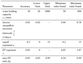
fit-ted to determine runoff, evapotranspiration and streamflow of a catchment. This is done for each catchment using the same optimization approach as in Orth et al. (2013), whereby the optimal set of parameters is determined as the set that yields the best fit between modelled and observed streamflow among 25 estimated sets (representing local maxima in the five-dimensional parameter space). This fit is evaluated as a correlation during July, August and September of all avail-able years to avoid an impact of snow, which is not included in the model. As in Orth et al. (2013), we use a correlation to determine the fit because our focus is on the simulation of the temporal evolution of soil moisture and streamflow rather than on their absolute amount (as the former is more relevant to represent memory characteristics. Table 1 sum-marises the accuracies with which the parameters are fitted (i.e. the step width for each parameter as applied in the op-timization procedure), their upper and lower limits as well as maxima and minima of the actual parameter values found for the catchments considered here (see Sect. 3). Note that in contrast to Orth et al. (2013), we apply here upper limits to the exponentsαandγ (15) and the water holding capacity cs (2000 mm) to accelerate the optimization process and to
prevent unreasonable fitted parameter values. 2.2 Computation of slopes
To quantify the impact of soil moisture on streamflow and ET, we use the slopes of the runoff and ET functions (Eqs. 2
Table 1.Overview of model parameter accuracies, boundaries and
the range of their respective estimates.
Lower Upper Minimum Maximum Parameter Accuracy limit limit value found value found
water holding 30 20 2000 50 890
capacity cs(mm)
inverse 0.02 0.02 – 0.04 0.78
streamflow recession timescale1
τ (1/days)
runoff 0.2 0 15 0.2 15
exponentα
ET exponent 0.03 0 – 0.03 3.87
γ
max ET 0.03 0.03 0.99 0.24 0.99
ratioβ0
and 3) normalised with precipitation and net radiation, re-spectively. These slopes are catchment-specific and depend only on the soil moisture content and on the fitted param-eters. They are computed as follows: for every daily soil moisture value that occurs between May and September over the whole considered time period (see Sect. 3) in a particu-lar catchment we compute the respective slopes of the nor-malised runoff and ET functions from their derivations with respect to soil moisture. Then we take the mean of all the slopes to derive mean slopes for the runoff and ET function of each catchment. These mean slopes represent the average sensitivity of runoff and ET to soil moisture in the respective catchments.
As described and illustrated later in Sect. 4.2, the runoff and ET function slopes are important variables for the soil moisture-streamflow and soil moisture-ET coupling strengths. For instance, a slope of zero implies no impact of soil moisture, whereas a high slope implies that soil moisture changes are readily translated into changes of streamflow or ET.
2.3 Computation of memory
To determine the persistence of soil moisture, streamflow and ET produced by the simple water-balance model, we cal-culate the respective memory as an inter-annual correlation over a particular lag (see Koster and Suarez, 2001; Senevi-ratne and Koster, 2012): for a given quantity, the estimates of daynfrom all years are correlated with the estimates of
dayn+tlagfrom all years. To derive representative memory
ρ wn, wn+tlag
=
1
tend−tstart+60−tlag
tend+30−tlag
X
i=tstart−30
ρ wi, wi+tlag
(7)
wheretstartandtendrefer to the respective start and end dates
of the considered half-monthly time period. Starting 30 days prior to the beginning of the half-monthly interval and finish-ing 30-tlagdays after the end of the half-monthly period, we
obtain a number of correlations of which we take a trimmed average (not shown in Eq. 7). We avoid the 10 % highest and 10 % lowest values, as in Orth et al. (2013) to yield a rep-resentative memory estimate for the particular half-monthly period.
In order to study the connection between soil moisture memory and the memory of streamflow and ET, respectively, we consider in the following 30-day-lag memories that are computed as described above for all quantities. To assess the impact of the investigated time scale, we perform the same analysis using monthly averaged data from which we com-pute the respective 1-month-lag memories.
2.4 Computation of persistence time scales
While memory is considered as lag correlation in the previ-ous subsection and previprevi-ous studies (e.g. Koster and Suarez, 2001; Orth and Seneviratne, 2012), we relate the memories of soil moisture, streamflow and ET in this study also to per-sistence time scales. This is more easily interpretable and allows us to study the respective memories under different hydrological conditions.
For the computation of this persistence time scale we pro-ceed as follows: (i) we define “normal” conditions at a partic-ular day as those differing at most by one standard deviation (computed over the values of that day from all years) from the mean of that day over all years; (ii) we choose deviations of 1.33 and 1.66 standard deviations from the mean as thresh-olds for medium and strong anomalies, respectively; (iii) we select all days of the time series between May and September that exceed a threshold and calculate for each day the delay until which the quantity of interest recovers to normal con-ditions; (iv) finally, we take the mean of all the durations to derive a mean persistence of anomalous conditions once they have exceeded a certain threshold. Note that the time frame of May through September (point iii above) is chosen in or-der to avoid cold season impacts such as snow and land cover changes. Comparing the persistence time scale to respective memories expressed as lag correlations, we can relate these correlations to mean recovery times from respective anoma-lies determined by a chosen threshold.
2.5 Coupling of streamflow and evapotranspiration to soil moisture
As this study is investigating the propagation of memory from soil moisture to streamflow and ET, it is necessary to assess the extent to which streamflow and ET are driven by soil moisture. For this purpose, we introduce a measure of the coupling strength between soil moisture and streamflow, or soil moisture and ET, respectively. We define the coupling strength between soil moisture and streamflow (hereafter re-ferred to as soil moisture-streamflow coupling strength) as their correlation,ρ (Qn, wn). Similarly, to measure the
cou-pling strength between soil moisture and ET (hereafter re-ferred to as soil moisture-ET coupling strength), we use
ρ (En, wn).
The computation of these correlations is performed in a similar way as in Eq. (7). Instead of correlating estimates of a given quantity at dayn from all years with the estimates
of dayn+tlagfrom all years, we correlate estimates of one
quantity at daynfrom all years with estimates of the other
quantity at the same daynof all years. Similar to memory,
the coupling strengths are also computed as representative estimates for half-monthly periods.
Using these estimates we can determine and compare the respective coupling strengths with each other, in different seasons, and across the various catchments (see Sect. 3).
3 Data
In order to derive a spatially distributed evaluation of soil moisture, streamflow and ET memory across Europe we ap-ply the simple water-balance model to near-natural catch-ments (i.e. catchcatch-ments with negligible human impact) lo-cated throughout Europe. The corresponding streamflow data stem from a dataset compiled by Stahl et al. (2010), who collected data from the European water archive (http://grdc. bafg.de, checked on 16 July 2012), from national ministries and meteorological agencies, as well as from the WATCH project (http://www.eu-watch.org, checked on 16 July 2012). The simple model uses precipitation and radiation infor-mation as an input. We use satellite-measured net radiation from the NASA/GEWEX SRB project (http://eosweb.larc. nasa.gov/PRODOCS/srb/table_srb.html, checked on 16 July 2012). The precipitation data was obtained from the E-OBS dataset (http://eca.knmi.nl, checked on 16 July 2012), which is an interpolation of rain gauge measurements on a regular grid across Europe. It was developed by the ENSEMBLES project (http://ensembles-eu.metoffice.com, checked on 16 July 2012).
−10 0 10 20 30
35
40
45
50
55
60
65
70
longitude
latitude
1 2 4 8
mean daily streamflo
w (mm)
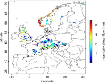
Fig. 1.The coloured large dots indicate the locations of the selected 100 catchments. The colour coding indicates the mean daily stream-flow between May and September. The smaller black dots indicate the locations of the remaining catchments of the Stahl et al. (2010) dataset, as considered for the validation of streamflow (memory) in Sect. 4.1. The arrow points to the Le Saulx catchment later consid-ered in Sect. 4.2.
3.1 Selection of catchments
Given the large number of>400 catchments contained in the
Stahl et al. (2010) dataset, we had to select a subset for two reasons: (i) the parameter fitting procedure (Sect. 2.1.3) is computationally demanding and (ii) in a few catchments the fitting procedure did not work well, as seen from a low corre-lation between modelled and observed streamflow (probably due to impacts of snow, which is not included in the model). Running the parameter fitting procedure with 5 instead of 25 iterations (see Sect. 2.1.3) for all catchments to reduce the computational effort (thereby increasing the risk that the re-sulting parameter set is only a local instead of a global max-imum in the five-dimensional parameter space), we selected 100 catchments for this study, for which the streamflow op-timization (see Sect. 2.1.3) yielded the highest correlations. For the selected 100 catchments we then performed the pa-rameter fitting procedure another 20 times to ensure that the global optimum of the parameters is found. Corresponding information on name, coordinates, river, size, altitude and mean streamflow of the considered catchments is provided in Appendix A. Their locations together with their mean daily streamflow are displayed in Fig. 1. The catchments are well distributed across the continent, except for the south-east, thus allowing an analysis of persistence across a large re-gion. As can be inferred from Table 1, the range of the fitted parameter values is larger compared to Orth et al. (2013) as we consider many more catchments, which are moreover dis-tributed over a much wider area and across a broader range of climate regimes.
4 Results
In this section, we first present an evaluation of the simple model’s simulated streamflow and its memory in the con-sidered catchments, followed by a case study to illustrate the model behaviour under different hydrological conditions. Thereafter we investigate the connection between soil mois-ture memory on the one hand and streamflow and ET mem-ory on the other hand, including an identification of the main drivers for these relationships. In the last part of this sec-tion, we present a different view on memory: we quantify its strength as a recovery time from anomalous conditions and investigate its variations with extreme conditions.
4.1 Evaluation of modelled streamflow
The employed water-balance model was earlier validated at 13 Swiss catchments in Orth et al. (2013), with a focus on soil moisture memory,ρ wn, wn+tlag
. However, the present
study also focuses on streamflow memory,ρ Qn, Qn+tlag
,
and considers a much wider region that covers a large frac-tion of Europe. Hence, we provide here an evaluafrac-tion of the performance of the simple water-balance model with respect to its representation of mean streamflow andρ Qn, Qn+tlag
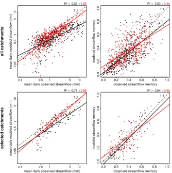
at the investigated catchments. To allow an independent val-idation, we consider monthly averages for June and October in all catchments as these months are not part of the optimiza-tion period in which the model is calibrated (see Sect. 2.1.3). The results are displayed in Fig. 2. Note that we investigate here the subset of catchments described in Sect. 3.1 as well as the totality of the 430 catchments of the Stahl et al. (2010) dataset. This allows us to show that the simple water balance model displays a meaningful performance in the catchments we disregard for the remainder of this study. Note that for the excluded catchments we performed the parameter fitting procedure with 5 instead of 25 iterations (see Sect. 2.1.3) to reduce the computational effort (thereby increasing the risk that the resulting parameter set is only a local instead of a global maximum in the five-dimensional parameter space).
mean daily observed streamflow (mm)
mean daily modeled streamflo
w (mm)
0.1 0.5 1 5 10
0.05
0.5
1
5
10
R² = 0.53 / 0.55
1:1
all catc
hments
0.0 0.2 0.4 0.6 0.8 1.0
0.0
0.2
0.4
0.6
0.8
1.0
observed streamflow memory
modeled streamflo
w memor
y
1:1
R² = 0.53 / 0.42
mean daily observed streamflow (mm)
mean daily modeled streamflo
w (mm)
0.1 0.5 1 5 10
0.05
0.5
1
5
10
R² = 0.71 / 0.86
1:1
selected catc
hments
0.0 0.2 0.4 0.6 0.8 1.0
0.0
0.2
0.4
0.6
0.8
1.0
observed streamflow memory
modeled streamflo
w memor
y
1:1
R² = 0.64 / 0.59
Fig. 2. The left plots show modelled versus observed mean daily
streamflows for June (in black) and October (in red). Note the log-arithmic scale of both axes. The thick straight lines are fitted with least-squared regression,R2values shown on top are a result of this. The right plots show the same, only for mean monthly stream-flow memoryρ Qn, Qn+15 days. The upper row shows results for all 441 catchments, the lower row only contains the selected catch-ments.
has been used for the calibration of the model. As shown on the right hand side of Fig. 2, the streamflow memory
ρ Qn, Qn+15 daysis well captured by the model for most
catchments, although the regression lines indicate a slight un-derestimation of highρ Qn, Qn+15 daysin both months. For
the same reason discussed above, the explained fraction of variance is slightly higher in October compared to June. Note that the explained fraction of variance, R2, is higher (0.8)
when comparing ρ Qn, Qn+15 days
of the selected
catch-ments, averaged from May–September (as used in Sects. 4.3 and 4.4). The agreement between modelled and observed
ρ Qn, Qn+15 days
is better for the selected, reduced number
of catchments than for the totality of catchments, indicating that the quality of the modelledρ Qn, Qn+15 daysdepends
to some extent on the goodness of the streamflow optimiza-tion. This supports our selection of a subset of catchments (see Sect. 3.1), as it shows that we can assume that the model captures hydrological processes better (and therefore also the persistence of the involved quantities) if the calibration al-lows to better reproduce observed streamflow.
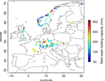
In order to further validate the simple water balance model and the parameter fitting procedure, we display the fitted water holding capacities in Fig. 3. The fitted values fall in a physically meaningful range. Furthermore, in many re-gions we find similar water holding capacities for nearby
catchments, underlining the robustness of the parameter fit-ting approach. Some few exceptions are probably due to the heterogeneous nature of soil and land cover characteristics. Additionally, there are large-scale variations; in central Ger-many and across France the storage capacity tends to be higher, whereas in the Alps and at the Norwegian coast we find low water holding capacities.
4.2 Case study – Le Saulx catchment
−10 0 10 20 30
35
40
45
50
55
60
65
70
longitude
latitude
50 100 200 400 800
fitted w
ater holding capacity (mm)
Fig. 3. Fitted water holding capacities for the selected catchments. Note the logarithmic scale of the colour-coding.
Keeping these relationships in mind, the lower part of Fig. 4 displays the evolution of modelled soil moisture, streamflow and ET during the April–July 1998 dry-down pe-riod, together with the corresponding precipitation and net radiation forcing. The dashed red line indicating the ob-served streamflow evolution compares well with the mod-elled streamflow in terms of the temporal evolution (on which we focus, see Sect. 2.1.3), pointing out a reasonable performance of the model. The first month, April, is rather wet (high precipitation) and cloudy (low net radiation). Con-sequently, the streamflow is high, responds strongly to pre-cipitation, and its evolution corresponds well with the soil moisture evolution, underlining the high sensitivity to soil moisture discussed above (as soil moisture is still below the water holding capacity). In contrast to streamflow, ET is lower, mostly driven by net radiation, and displays a low sensitivity to changes in soil moisture. During May and June the catchment experienced mostly sunny and dry conditions (high net radiation), only interrupted by low to medium pre-cipitation in late May and early June. Correspondingly the soil dries out remarkably. The streamflow therefore decreases to almost zero, showing almost no response to the precipita-tion and the following slight increase of soil moisture. This illustrates the decoupling of streamflow from soil moisture under dry conditions. On the other hand, ET is compara-tively high and roughly follows the strong soil moisture de-crease and the subsequent stabilization, although net radia-tion is still the main driver, as a maximum in net radiaradia-tion in the second half of June causes a pronounced maximum in ET (even if soil moisture is decreasing). Finally, in July soil moisture has decreased to very low levels such that the ET level is lower and, more importantly, despite strong day-to-day variations in net radiation, the ET evolution corresponds more closely to soil moisture, but still also to net radiation (keeping in mind that the ET time series is smoothed with a 7-day running mean).
0 50 100 150 200
Soil Moisture (mm)
Q/P and ET/Rnet
0
0.25
0.5
0.75
1
Q/P fitted ET/Rnet fitted
a)
April May June July
1998
0 5 10 15 20 80 100 120 140 160
0 1 2 3 0
40 80 120 160 200
Net Radiation (W/m2)
Soil Moisture (mm)
Precipitation (mm/da
y) ET (mm/da
y)
&
Streamflo
w (mm/da
y)
Net Radiation
Soil Moisture
Streamflow
Evapotranspiration
Precipitation
b)
Fig. 4. (a)Fitted normalised runoff (Eq. 2) and ET (Eq. 3) functions for the Le Saulx catchment in eastern France (indicated by an arrow in Fig. 1). The background histogram shows the relative abundance of soil moisture contents between April and October.(b)Time se-ries of forcing (net radiation at the top, precipitation at the bottom) and according output of the simple model (soil moisture, stream-flow and ET in between the forcings) from the Le Saulx catchment during a pronounced dry-out period from April until July 1998. The dashed red line indicates the evolution of the observed streamflow. The fitted water holding capacity for this catchment is 170 mm, such that the normalised streamflow function reaches 1 at this soil mois-ture content. Note that the ET time series has been smoothed to fa-cilitate the readability of the graph such that each value represents the average of the current day, the three preceding days and the three following days.
4.3 Propagation of soil moisture memory
mean = 0.36
−10 0 10 20 30
Daily data
latitude
Soil Moisture Memor
y
40 50 60 70
mean = 0.5
−10 0 10 20 30
Monthly data
40 50 60 70
mean = 0.13
latitude
Streamflo
w Memor
y
40 50 60 70
mean = 0.28
40 50 60 70
mean = 0
−10 0 10 20 30
longitude
latitude
Ev
apotranspiration Memor
y
40 50 60 70
mean = 0.07
−10 0 10 20 30
longitude
40 50 60 70
0.0 0.2 0.4 0.6 0.8 1.0
lag−correlation
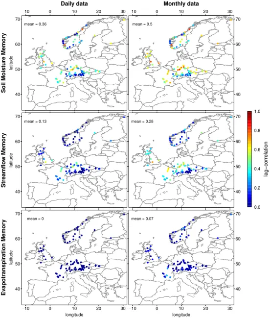
Fig. 5. Geographical distribution of mean May–September memories of soil moisture (ρ wn, wn+lag
, upper row), streamflow
(ρQn, Qn+tlag
, centre row) and ET (ρ En, En+lag
, lower row) for daily and monthly averaged data (all memories computed for a
lag of 30 days (daily data) or 1 month (monthly data)) computed as described in Sect. 2.3.
4.3.1 Memory of soil moisture, streamflow and evapotranspiration
Figure 5 displays the 30-day-lag memories of soil mois-ture (ρ wn, wn+30 days), streamflow (ρ Qn, Qn+30 days)
and ET (ρ En, En+30 days) computed from daily data in all
catchments as compared to the respective 1-month-lag mem-ories (e.g. ρ (wn, wn+1 month)) computed from monthly
av-eraged data. The memory patterns derived from daily and monthly data are very similar. The 1-month-lag memories are higher, which results from the aggregation of the data that minimises the impact of day-to-day variations in the me-teorological forcing.
As reported in numerous earlier studies (e.g. Delworth and Manabe, 1988; Entin et al., 2000; Robock et al., 2000; Koster and Suarez, 2001; Orth and Seneviratne, 2012) we find considerable persistence in soil moisture in almost all catchments. Largestρ wn, wn+30 days
is found across
Cen-tral Europe (Germany, eastern France). We find generally
low ρ wn, wn+30 days in mountainous areas (Alps, Massif
central, Scandinavian mountains). Note that these large-scale patterns correspond with the spatial distribution of the fitted water holding capacities shown in Fig. 3, pointing out the im-portance of the storing capacity forρ wn, wn+30 days. Also
(Germany, Norway). This highlights the importance of lo-cal soil and vegetation characteristics in comparison to the impact of the particular climate regime.
Interestingly, for streamflow we find medium memory in many parts of Europe, especially in the Central Europe and in the South-West, whereρ wn, wn+30 daysis also highest.
Apart from these rather dominant large-scale variations we find small-scale variations, as can be seen from the partly high memory differences between nearby catchments in cen-tral Europe, pointing out some importance of the role of local catchment characteristics also for ρ Qn, Qn+30 days
.
Fig-ure 5 shows moreover some memory in ET only for monthly data in some catchments in southern France. Possible reasons for this feature will be discussed in the following subsections.
4.3.2 Forcing memories and variabilities
As described in Sect. 2.1.1, streamflow depends on runoff (and therefore on soil moisture and precipitation) and on the delay time scaleτ (Eq. 5). Therefore,ρ Qn, Qn+tlag
may
result from propagatingρ wn, wn+tlag
, but it is additionally
induced by the delay time scale. ET depends on soil moisture and net radiation (Eq. 2) and hence its memory may stem fromρ wn, wn+tlag
or
ρ Rn, Rn+tlag
.
For daily data, net radiation memory and precipitation memory are negligible. Therefore, ET memory results al-most entirely from soil moisture memory, whereas stream-flow memory is additionally impacted by the delay time scale. On the monthly time scale, however, we find small but no longer negligibleρ Rn, Rn+tlag
or
ρ Pn, Pn+tlag
which
may be caused by persisting patterns of the atmospheric cir-culation. Associated with that the forcing variabilities de-crease towards longer time scales as day-to-day variations are averaged out. Note that the variability of radiation decreases more strongly than that ofPn∗as it already incorporates the
joint impact of many daily precipitation sums.
4.3.3 Controls of memory propagation
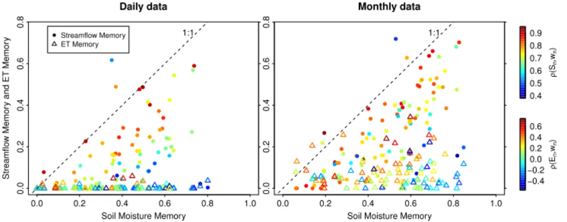
To assess the relationship of soil moisture memory,
ρ wn, wn+tlag
, with streamflow memory,
ρ Qn, Qn+tlag
,
and ET memory, ρ En, En+tlag
, a scatter plot of
ρ Qn, Qn+tlag
and
ρ En, En+tlag
from all selected
catch-ments as a function of the correspondingρ wn, wn+tlag
is
displayed in Fig. 6. Every point and every triangle represent one catchment. The left plot is based on daily data and shows 30-day-lag memories whereas the right plot is based on monthly data and shows 1-month-lag memories. In agree-ment with Fig. 5, this analysis shows that ρ En, En+tlag
are generally lower thanρ Qn, Qn+tlag
. With the help of
the dashed identity line we find thatρ Qn, Qn+tlag
seems
to be limited by the corresponding ρ wn, wn+tlag
, which
suggests thatρ Qn, Qn+tlag
to some extent originates from
ρ wn, wn+tlag
. However, in two catchments
ρ Qn, Qn+tlag
clearly exceeds the estimatedρ wn, wn+tlag
. This is because
ρ Qn, Qn+tlag
is not solely induced by
ρ wn, wn+tlag
,
but it may also be generated through the transformation of runoff into streamflow (Eq. 5), i.e. by (slow) transport of runoff water to the stream and in the stream towards the stream gauge station; the corresponding delay time scale that is among the longest in these two catchments. Depending on the size of the catchment, this may remove some of the variability of the runoff signal on the daily time scale.
Using colour coding, Fig. 6 shows the respective soil moisture-streamflow and soil moisture-ET coupling strengths (ρ (Qn, wn) and ρ (En, wn), respectively, see
Sect. 2.5). The streamflow memories ρ Qn, Qn+tlag
are
found to be dependent on ρ (Qn, wn). Almost all
catch-ments that show comparatively high ρ Qn, Qn+tlag
, also
show comparatively highρ (Qn, wn)together with relatively
high soil moisture memory ρ wn, wn+tlag
. This supports
the above-described propagation ofρ wn, wn+tlag
. For ET
memoryρ En, En+tlag
, the link to
ρ (En, wn)is less clear,
nonetheless most of the catchments with comparatively high
ρ En, En+tlag
display a higher
ρ (En, wn)at the same time.
In most catchments,ρ (En, wn)is weaker than ρ (Qn, wn),
which explains whyρ Qn, Qn+tlag
exceeds
ρ En, En+tlag
.
Whereas the streamflow memory ρ Qn, Qn+tlag
in-creases only slightly from daily to monthly time scales, the ET memoryρ En, En+tlag
increases much stronger. This is
because ρ (En, wn) increases stronger than ρ (Qn, wn) for
most catchments, thanks to the strong reduction in radiation variability with increasing time scale (see Sect. 4.3.2). These findings highlight the importance of the time scale used in memory considerations. Although the forcing memories are no longer negligible on the monthly time scale (Sect. 4.3.2), Fig. 6 illustrates thatρ Qn, Qn+tlag
and
ρ En, En+tlag
on
the monthly time scale are mostly controlled by soil moisture memoryρ wn, wn+tlag
and the respective coupling strength,
ρ (En, wn)orρ (Qn, wn), like on the daily time scale.
When computing the memory of the evaporative fraction
En
Rn
instead of ET on the daily time scale (not shown) we find a far stronger memory which is of similar order as for
ρ wn, wn+tlag
, underlining the strong weakening impact of
daily net radiation variability onρ En, En+tlag
. Similarly,
the memory of Run
Pn
is similar toρ wn, wn+tlag
on the daily
time scale (not shown), and therefore stronger than that of streamflow, which underlines the weakening impact of day-to-day precipitation variability.
Summing up, we have shown in this section that the streamflow and ET memories, ρ Qn, Qn+tlag
and
ρ En, En+tlag
depend on (i) soil moisture memory
ρ wn, wn+tlag
, which acts to some extent as an upper limit,
0.0 0.2 0.4 0.6 0.8 1.0
0.0
0.2
0.4
0.6
0.8
Daily data
Soil Moisture Memory Streamflow Memory
ET Memory
Streamflo
w Memor
y and ET Memor
y 1:1
0.0 0.2 0.4 0.6 0.8 1.0
0.0
0.2
0.4
0.6
0.8
Monthly data
Soil Moisture Memory 1:1
0.4 0.5 0.6 0.7 0.8 0.9
ρ
(S
n
,w
n
)
−0.4 −0.2 0.0 0.2 0.4 0.6
ρ
(E
n
,w
n
)
Fig. 6. Streamflow (dots) and ET (triangles) memoriesρ
Qn, Qn+tlag
andρ En, En+lag
, respectively, of all selected catchments plotted
versus the corresponding soil moisture memoriesρ wn, wn+lag
for daily and monthly averaged data (all memories computed for a lag of
30 days (daily data) or 1 month (monthly data)). The colour coding denotes the strength of the soil moisture-streamflow couplingρ (Qn, wn) and the soil moisture-ET couplingρ (En, wn), respectively (see Sect. 2.5).
Fig. 7. Schematic view of propagation of soil moisture memory to streamflow memory and ET memory. Red arrows denote positive impacts, blue arrows show negative impacts. Only dependencies in-vestigated in this study are shown.
memory ρ Qn, Qn+tlag
may be generated by the delay
time scale τ reflecting the conversion of runoff to
stream-flow. A schematic view of these dependencies is presented in Fig. 7, with positive relationships denoted by red ar-rows and negative relationships shown with blue arar-rows. It illustrates that the forcing memory not only supports
ρ Qn, Qn+tlag
and
ρ En, En+tlag
, but also the soil moisture
memoryρ wn, wn+tlag
itself (Orth and Seneviratne, 2012).
Moreover the scheme includes controls of ρ (Qn, wn) and
ρ (En, wn), which are discussed in the following subsection
together with a further discussion of Fig. 7.
4.4 Soil moisture-streamflow and soil moisture-ET coupling
4.4.1 Geographical distribution
Figure 8 displays the geographical distribution of the two coupling strengths introduced in Sect. 2.5 and computed with daily and monthly averaged data, respectively. The geograph-ical patterns appear to be independent of the applied av-eraging time scale. As seen previously for the streamflow and ET memories, the soil moisture-streamflow coupling strengths are similar for different time scales whereas the (ab-solute values of the) soil moisture-ET coupling strengths in-crease significantly in many catchments with increasing (i.e. daily to monthly) time scale. This is furthermore reflected in a clear increase of the standard deviation of all respec-tive soil moisture-ET coupling strengths from the daily to the monthly time scale.
The soil moisture-streamflow couplingρ (Qn, wn)is
over-all clearly stronger than the soil moisture-ET coupling
ρ (En, wn). It is comparatively weak in coastal areas (Great
Britain, Norway) and rather strong in flat, continental regions (Germany, France). However, in coastal areas around the Baltic sea (Denmark, Estonia, Finland) there is no reduction inρ (Qn, wn). Overall, large-scale variations are dominant,
although in some regions (e.g. Norway and Great Britain) relatively large differences are found for some nearby catch-ments.
For the soil moisture-ET coupling,ρ (En, wn), small-scale
variations are more prominent than large-scale variations, especially on the monthly time scale. In southern France the coupling is particularly strong due to prevailing the dry regime in that region. Under such a regime, soil moisture is rather low and the ET function slope is rather high (see Sect. 4.2). Negativeρ (En, wn), which is seen at the monthly
mean = 0.66 st.dev. = 0.1
−10 0 10 20 30
Daily data
latitude
ρ
(S
n
,w
n
)
40 50 60 70
mean = 0.76 st.dev. = 0.1
−10 0 10 20 30
Monthly data
40 50 60 70
mean = 0.1 st.dev. = 0.12
−10 0 10 20 30
longitude
latitude
ρ
(E
n
,w
n
)
40 50 60 70
mean = 0.14 st.dev. = 0.3
−10 0 10 20 30
longitude
40 50 60 70
−1.0 −0.5 0.0 0.5 1.0
ρ
(Sn ,wn
) and
ρ
(E
n
,w
n
)
Fig. 8. Geographical distribution of mean May–September soil moisture-streamflow (upper row) and soil moisture-ET (lower row) coupling strengthsρ (Qn, wn)andρ (En, wn), respectively, for daily and monthly averaged data. Respective strengths are shown through the colour coding. In the upper left corner of each plot the mean and standard deviation over the selected catchments are displayed.
Europe, can be explained with very low slopes of the fitted ET ratio functions in these catchments. As a consequence ET depends almost entirely on net radiation there, which is usually negatively related with precipitation and hence soil moisture.
4.4.2 Controls
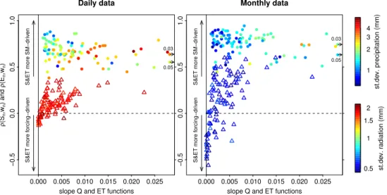
Having shown that streamflow and ET memory are origi-nating from soil moisture memory and are furthermore con-trolled by the respective soil moisture-streamflow and soil moisture-ET coupling strengths, we analyse here the two coupling strengths themselves. Thereby we determine which climatic regime or catchment characteristics support or in-hibit memory propagation. As shown in Fig. 7, we investi-gate and identify two controls for the coupling strengths: (i) the sensitivity of runoff (normalised by precipitation) and ET (normalised by net radiation) to soil moisture as measured by the mean slopes of the corresponding functions (Eq. 2 and 3; see also example in Fig. 4), (ii) the variance of the forcing, i.e. of cumulative weighted precipitation (Pn∗, Eq. 6)
and net radiation (Rn). We consider here the influence of the
forcing variances on the translation of a soil moisture signal into streamflow and/or ET. For instance even if the respective
slope is high, the respective coupling strength may be re-duced by a high forcing variance.
Figure 9 shows the impact of both above-described drivers on the two coupling strengths for daily and monthly aver-aged data. Every point (streamflow) and every triangle (ET) represents one catchment. The respective slopes of the fitted runoff and ET functions are plotted on they axes and the
forcing variances can be read from the colour coding of the symbols.
Focusing on ET first, we find increasingρ (En, wn)with
increasing mean slope of the ET function on both time scales. The radiation variances are very similar in all catchments. When comparing the variances at different time scales, we find a clear reduction towards the longer, monthly time scale (see also Sect. 4.3.2). This is because day-to-day varia-tions are averaged out, which causes a stronger increase of
ρ (En, wn)with increasing slope of the ET function.
Interestingly, ρ (Qn, wn) does not increase with an
in-creasing slope of the runoff function, but instead decreases slightly on both considered time scales. Apart from the ef-fect of the slope,ρ (Qn, wn)is moreover controlled by the
variance of the atmospheric forcing (cumulative weighted precipitationP∗
n). Different precipitation variances cause a
0.000 0.005 0.010 0.015 0.020 0.025
−0.5
0.0
0.5
1.0
Daily data
slope Q and ET functions
ρ
(S
n
,w
n
) and
ρ
(E
n
,w
n
)
S&ET more SM−dr
iv
en
S&ET more f
orcing−dr
iv
en
0.03
0.05
0.000 0.005 0.010 0.015 0.020 0.025
−0.5
0.0
0.5
1.0
Monthly data
slope Q and ET functions
S&ET more SM−dr
iv
en
S&ET more f
orcing−dr
iv
en
0.03
0.05
1 2 3 4
st.de
v. precipitation (mm)
0.5 1 1.5
2
st.de
v. r
adiation (mm)
Fig. 9. Soil moisture-streamflow (dots) and soil moisture-ET (triangles) coupling strengths,ρ (Qn, wn)andρ (En, wn), respectively, plotted against the respective runoff and ET function slope (computed as described in Section 4.4.2) for daily and monthly averaged data. The colour coding denotes the variance of the weighted precipitation sum precipitation (P∗
n) and of radiation, respectively. All involved quantities computed as means from May–September. Points that do not fit with the range of thexand/oryaxis are also included together with an arrow pointing in the direction of their actual location and the true value displayed next to it.
slopes. The rather strong role of the precipitation variance forρ (Qn, wn)compared to the role of the radiation variance
for the soil moisture-ET coupling is due to the much larger spread of the precipitation variances between all catchments, as shown in the colour bars in Fig. 9. Note, however, that the displayed variance ofPn∗is not strictly a forcing variance, as Pn∗is determined in part by the delay time scaleτ(see Eq. 6),
which means consequently thatτ may impactρ (Qn, wn).
The scheme in Fig. 7 summarises all the relation-ships investigated above. It illustrates how ρ (Qn, wn) and
ρ (En, wn)feed back on soil moisture memory. The stronger
streamflow and ET respond to soil moisture, the more they tend to dampen initial soil moisture anomalies. For instance, a dry anomaly causes a decrease in streamflow and ET, whereas a wet soil moisture anomaly would cause a strong increase, especially in streamflow (see Fig. 4). The impact of the initial soil moisture anomaly for the subsequent soil moisture memory is discussed in Sect. 4.5. The variability of the forcings (precipitation and radiation) may weaken the streamflow and ET memory, but this effect only plays a role in case of low slopes of the runoff and ET functions, as seen especially for streamflow in Fig. 9.
4.4.3 Differences between soil moisture-streamflow and soil moisture-ET coupling
As discussed in Sect. 4.3.3, streamflow memory exceeds ET memory in almost all catchments on the daily time scale, and in most catchments on the monthly time scale. This is caused by the stronger coupling of streamflow to soil mois-ture (ρ (Qn, wn) > ρ (En, wn)) in most of the investigated
catchments, with the slope of the runoff function typically
exceeding that of the ET function. Additionally, the forc-ing variabilities play a role. As described in Sect. 4.3.3, they decrease with increasing time scale because day-to-day variations are averaged out, but the radiation variability de-creases more strongly, which explains why the ET memory increases more than the streamflow memory with increasing time scale.
The higher runoff function slopes and the consequently stronger impact of streamflow on soil moisture dynamics compared to the impact of ET on soil moisture dynamics are another reason for the considerable spread of the triangles in Fig. 9. Catchments with similar ET function slopes may have very different runoff function slopes that impact soil moisture dynamics differently, thereby causing differentρ (En, wn). It
should be noted that these results are likely dependent on the climatic region where the catchments are located, and that the considered catchments are mostly located in central and northern Europe, i.e. in rather radiation-limited conditions. 4.5 Relating memory to persistence time scales
35
45
55
65
Latitude
Soil Moisture
Strong dry anomalies
median = 25 days
Dry anomalies
median = 24 days
Wet anomalies
median = 17 days
35
45
55
65
Strong wet anomalies
median = 20 days
−10 0 10 20 30
Longitude
35
45
55
65
Latitude
Streamflo
w
median = 7 days
−10 0 10 20 30
Longitude
median = 5 days
−10 0 10 20 30
Longitude
median = 6 days
−10 0 10 20 30
Longitude
35
45
55
65
median = 7 days
10 30 50 70 90
Days
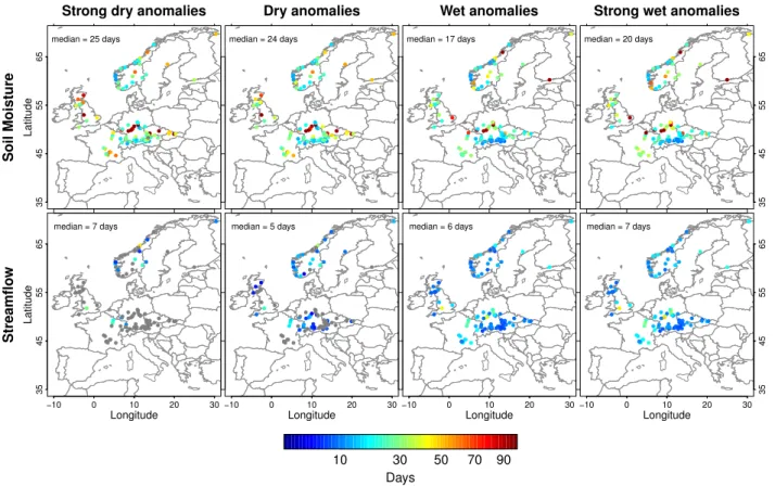
Fig. 10. Overview of mean durations to recover from (very) dry/wet conditions (1.33 and 1.66 standard deviations away from the respective daily mean of the respective quantity) to normal conditions (±1 standard deviation around the mean) for (modelled) soil moisture and streamflow. The results are based on daily data. In the upper left corner of each plot the median over all selected catchments is displayed. Gray colour indicates that no persistence can be computed because the applied threshold is almost never reached.
characteristics. For soil moisture we find median persistences over the considered catchments ranging from 17 to 25 days depending on the considered anomaly. For streamflow, the medians of the persistence time scales range between 5 and 7 days. Note that we do not investigate ET persistence here as there is almost no memory on the daily time scale (Fig. 5). We find that it takes generally longer to recover to normal conditions from strong anomalies than from medium anoma-lies. In other words, the stronger an initial anomaly, the more pronounced is the following memory effect. While this is not unexpected, it has important implications for the forecasts of extreme events, which should thus be more skillful than for close-to-normal conditions. Also previous studies reported an enhanced soil moisture memory following hydrological extreme conditions (Koster et al., 2010; Orth and Senevi-ratne, 2012). This impact of the initial soil moisture anomaly on the strength of the subsequent memory is also included in the schematic provided in Fig. 7.
We find that dry soil moisture anomalies persist longer, even if the difference to the persistence of wet anomalies is small in comparison to the absolute value of the persistences. The reason for this may be that the climate in most of the Eu-ropean catchments considered here is generally humid which
means that dry anomalies can be very extreme whereas wet anomalies are rather limited (as it cannot get much wetter). Unlike the soil moisture patterns, streamflow memory shows similar strength during dry and wet anomalies. While the propagating soil moisture memory supports the streamflow memory especially during dry anomalies, this result is due to the fact thatρ (Qn, wn)is stronger under wet conditions
(see Sect. 4.2), which allows a better propagation of the soil moisture memory to streamflow (see Sect. 4.3.3). Note that streamflow persistences for strong, dry anomalies could not be computed for all selected catchments, as in some catch-ments the respective threshold is only exceeded on very few days. This is because streamflow values rather follow an ex-ponential than a normal distribution.
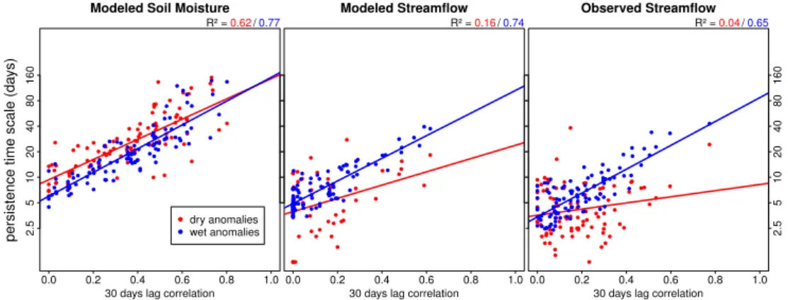
Figure 11 displays a comparison of memories computed as lag correlation and as persistence time scales. As above, we focus on soil moisture and streamflow, and we addition-ally investigate observed streamflow. The reasonably high
R2values of the linear fits indicate consistency between the
0.0 0.2 0.4 0.6 0.8 1.0
Modeled Soil Moisture
30 days lag correlation
2.5
5
10
20
40
80
160
R² = 0.62 / 0.77
dry anomalies wet anomalies
persistence time scale (da
ys)
0.0 0.2 0.4 0.6 0.8 1.0
Modeled Streamflow
30 days lag correlation R² = 0.16 / 0.74
0.0 0.2 0.4 0.6 0.8 1.0
Observed Streamflow
30 days lag correlation R² = 0.04 / 0.65
2.5
5
10
20
40
80
160
Fig. 11. Comparison of memory estimates computed as lag correlation and as persistence time scale (based on anomalies of 1.33 standard deviations from the mean) for modelled soil moisture and streamflow (left and middle) and observed streamflow (right). Red points refer to persistence time scales estimated from dry anomalies whereas blue points are derived from wet anomalies. The red and blue lines denote the respective linear least-squares fit. Note the logarithmic scale of the persistence time scale.
above. Figure 11 shows further that dry soil moisture anoma-lies persist longer than respective wet anomaanoma-lies, whereas for streamflow we find the opposite behaviour. The results for modelled and observed streamflow are similar, indicating a good representation of streamflow memory/persistence in the simple water balance model (which is not surprising, how-ever, as the model is calibrated with observed streamflow). The logarithmic scale of the persistence time scales indicates interestingly that persistence time scales increase exponen-tially for a linear increase in estimated lag correlation. This underlines the red noise character of soil moisture, which was already highlighted by Delworth and Manabe (1988). Note that the findings of this figure are robust, even if we consider persistence time scales related to other anomaly thresholds or lag correlations of other time lags.
5 Conclusions
Using data from 100 catchments located across Europe, we have shown that a simple water balance model is able to simulate realistic streamflow as well as realistic streamflow memory characteristics compared to observations, thereby expanding an earlier validation performed by Orth et al. (2013).
Further, this study investigated the relationship of stream-flow and ET memory to soil moisture memory. We showed that soil moisture memory to some extent serves as an upper bound for streamflow and ET memory. Furthermore, we de-fined measures of the coupling between soil moisture and streamflow, as well as between soil moisture and ET and found that their strengths determine the memory strength of streamflow and ET, respectively. These findings explain why one can infer that the memory propagates from soil
mois-ture to streamflow and ET as illustrated in Fig. 7. As stream-flow and ET are moreover driven by the meteorological forcing, also the (small) memories of cumulative weighted
precipitation and net radiation (only on the monthly time scale) play a (minor) role for the strength of their respective memories.
Comparing the results for daily and monthly time scales we generally find higher memory for monthly averaged data of soil moisture, streamflow and ET. This is due to the re-duced impact of the day-to-day variations of the meteorolog-ical forcing.
Figure 7 moreover displays the special role of the soil moisture-streamflow and soil moisture-ET coupling strengths. We show that the soil moisture-ET coupling is mostly controlled by the slope of the fitted (normalised) ET function whereas the soil moisture-streamflow coupling is strongly related to the variance of the weighted cumulative precipitation. In most catchments, the ET function slope is smaller than the runoff function slope, which is the main rea-son for the generally weaker coupling between soil moisture and ET, and the consequently lower ET memory compared to that of streamflow.
Table A1.Overview of catchments.
Catchment Gauging Size Mean Mean daily Catchment
(river) Country station (km2) altitude (m a.s.l.) streamflow (mm) centroid
Antiesen Austria Haging 165 512 1.35 48.3◦N 13.4◦E
Braunaubach Austria Hoheneich 292 580 0.60 48.8◦N 15.0◦E
Griesler Ache Austria St. Lorenz 122 732 2.99 47.8◦N 13.3◦E
Große Rodl Austria Rottenegg 226 703 1.19 48.3◦N 14.1◦E
Große Tulln Austria Siegersdorf 202 348 0.51 48.3◦N 15.9◦E
Leogangbach Austria Uttenhofen 112 2.14 47.4◦N 12.8◦E
Traun Austria Obertraun 334 1078 5.39 47.6◦N 13.7◦E
Otava Czech Republic Rejtejn 334 1025 2.22 49.1◦N 13.5◦E
Svratka Czech Republic Borovnice 128 0.97 49.7◦N 16.2◦E
Teplá Vltava Czech Republic Lenora 176 1018 1.47 48.9◦N 13.8◦E
Volynka Czech Republic Nemetice 383 728 0.63 49.2◦N 13.9◦E
Vantaa Finland Oulunkylä 1680 78 0.90 60.2◦N 25.0◦E
L’Aisne France Mouron 2239 208 0.95 49.3◦N 4.8◦E
L’Ance Du Nord France St-Julien-D’ance (Laprat) 354 995 1.01 45.3◦N 3.9◦E
Le Bes France St-Juery 283 1200 2.10 44.8◦N 3.1◦E
La Colagne France St-Amans (Ganivet) 89 1286 1.30 44.7◦N 3.4◦E
Le Doubs France Goumois 1060 992 2.36 47.3◦N 7.0◦E
La Drome France Luc-En-Diois 194 1014 1.02 44.6◦N 5.4◦E
La Loire France Bas-En-Basset 3234 968 0.90 45.3◦N 4.1◦E
La Moselle France St-Nabord (Noir Gueux) 633 720 3.35 48.1◦N 6.6◦E
Le Saulx France Vitry-En-Perthois 2109 264 1.12 48.7◦N 4.6◦E
La Seine France Bar-Sur-Seine 2344 320 0.94 48.1◦N 4.4◦E
La Sioule France St-Priest-Des-Champs (Fades-Besserve) 1305 781 1.08 46.0◦N 2.8◦E
La Tardes France Evaux-Les-Bains 854 507 0.84 46.2◦N 2.4◦E
La Truyere France Malzieu-Ville (Le Soulier) 582 1122 1.13 44.8◦N 3.3◦E
La Truyere France Neuveglise (Grandval) 1803 1069 1.17 44.9◦N 3.1◦E
Aitrach Germany Lauben 308 732 1.52 47.9◦N 10.0◦E
Apfelstädt Germany Ingersleben 371 449 0.60 50.9◦N 11.0◦E
Attel Germany Anger 244 523 1.39 48.0◦N 12.2◦E
Brugga Germany Oberried-Ibrech 40 989 3.41 47.9◦N 8.0◦E
Dhron Germany Papiermühle 170 489 0.95 49.8◦N 6.9◦E
Elsava Germany Rück 145 356 0.72 49.8◦N 9.2◦E
Engnitz Germany Hüttengrund 46 654 2.08 50.4◦N 11.2◦E
Gaissa Germany Hoerrmannsberg 212 457 1.30 48.7◦N 13.4◦E
Grosse Ohe Germany Schönberg 82 811 2.13 48.8◦N 13.4◦E
Grosser Regen Germany Zwiesel 177 886 2.52 49.0◦N 13.2◦E
Helme Germany Sundhausen 201 255 0.76 51.5◦N 10.8◦E
Kinzig Germany Schwaibach 964 600 2.16 48.4◦N 8.0◦E
Kollbach Germany Deggendorf 36 1.73 48.8◦N 13.1◦E
Lahn Germany Biedenkopf 309 477 1.60 50.9◦N 8.5◦E
Lohr Germany Partenstein 217 400 1.20 50.0◦N 9.5◦E
Mindel Germany Offingen 951 595 1.14 48.5◦N 10.4◦E
Mitternacher Oh Germany Eberhardsreuth 114 663 1.55 48.8◦N 13.4◦E
Osterbach Germany Röhrnbach 121 645 1.88 49.0◦N 13.2◦E
Reschwasser Germany Unterkashof 61 967 2.69 48.9◦N 13.5◦E
Rodach Germany Streitmühle bei Due 55 633 1.55 50.4◦N 11.5◦E
Rottach Germany Rottach 31 1159 2.88 47.7◦N 11.8◦E
Saalach Germany Unterjettenberg Rech 760 1211 3.34 47.7◦N 12.8◦E
Schwarzwasser Germany Aue1 362 745 1.51 50.6◦N 12.7◦E
Sinn Germany Mittelsinn 461 456 1.19 50.2◦N 9.6◦E
Steinacher Ache Germany Fallmuehle 22 1355 3.73 47.6◦N 10.5◦E
Stoisser Ache Germany Piding 50 738 2.08 47.8◦N 12.9◦E
Tiroler Achen Germany Staudach 944 1139 3.21 47.8◦N 12.5◦E
Traun Germany Stein Bei Altenmarkt 378 850 2.85 48.0◦N 12.6◦E
Uessbach Germany Peltzerhaus 176 410 0.84 50.1◦N 7.1◦E
Ulster Germany Guenthers 182 598 1.38 50.7◦N 10.0◦E
Untere Steinach Germany Oberhammer 67 576 1.44 50.2◦N 11.5◦E
Vils Germany Pfronten Ried 110 1369 3.78 47.6◦N 10.6◦E
Weisser Regen Germany Koetzing 226 692 1.72 49.3◦N 13.0◦E
Wertach Germany Biessenhofen 442 882 2.44 47.8◦N 10.7◦E
Weschnitz Germany Lorsch 383 214 0.71 49.7◦N 8.6◦E
Table A1.Continued.
Catchment Gauging Size Mean Mean daily Catchment
(river) Country station (km2) altitude (m a.s.l.) streamflow (mm) centroid
Årgårdselv Norway Øyungen 230 316 4.51 64.2◦N 11.1◦E
Engesetelev Norway Engsetvatn ndf 41 206 4.92 62.5◦N 6.6◦E
Etna Norway Etna 565 925 1.44 61.0◦N 9.6◦E
Etneelv Norway Stordalsvatn 140 611 9.09 59.7◦N 6.0◦E
Flisa Norway Knappom 1655 414 1.38 60.6◦N 12.0◦E
Forra Norway Høggås bru 458 525 3.77 63.5◦N 11.4◦E
Fusta Norway Fustvatn 520 472 5.58 65.9◦N 13.3◦E
Glomma Norway Atnasjø 468 1140 1.85 61.9◦N 10.2◦E
Guddalselva Norway Nautsundvatn 214 436 7.17 61.3◦N 5.4◦E
Jondalselv Norway Jondal 150 569 1.73 59.7◦N 9.6◦E
Kløvtveitelv Norway Kløvtveitvatn 5 466 11.06 61.0◦N 5.3◦E
Lygna Norway Tingvatn 265 564 5.80 58.4◦N 7.2◦E
Moelv Norway Salsvatn 435 285 5.18 64.7◦N 11.5◦E
Nordelva Norway Krinsvatn 210 435 5.42 63.8◦N 10.2◦E
Ogna Norway Helleland 75 336 6.79 58.5◦N 6.2◦E
Øren Norway Øren 151 264 4.05 62.8◦N 7.7◦E
Oselv Norway Røykenes 55 328 8.63 60.3◦N 5.4◦E
Strandå Norway Strandå 27 212 5.89 67.5◦N 14.9◦E
Tovdalselv Norway Austenå 310 752 3.01 58.8◦N 8.1◦E
No name Norway Karpelv 129 194 1.72 69.7◦N 30.4◦E
Biely Vah Slovakia Vychodna 106 1055 1.26 49.0◦N 19.9◦E
Kysuca Slovakia Cadca 492 647 1.46 49.4◦N 19.0◦E
Poprad Slovakia Poprad-Matejovce 311 1001 1.13 49.1◦N 20.3◦E
Rajcianka Slovakia Poluvsie 243 706 1.18 49.1◦N 18.7◦E
Dalelven Sweden Ersbo 654 728 3.34 61.3◦N 13.0◦E
Moelven Sweden Anundsjön 1457 283 1.10 63.4◦N 18.3◦E
Kleine Emme Switzerland Littau 78 2.00 47.5◦N 8.9◦E
Murg Switzerland Waengi 477 662 2.79 47.1◦N 8.3◦E
Allan Water United Kingdom Kinbuck 172 245 3.07 56.2◦N 3.9◦W
Coln United Kingdom Bibury 107 181 1.12 51.8◦N 1.8◦W
Cree United Kingdom Newton Stewart 368 243 3.77 55.0◦N 4.5◦W
Dart United Kingdom Austins Bridge 249 327 3.91 50.5◦N 3.8◦W
Dee United Kingdom Woodend 1394 512 2.46 57.1◦N 2.6◦W
Kinnel Water United Kingdom Redhall 78 245 3.45 55.2◦N 3.4◦W
Nith United Kingdom Friars Carse 812 293 3.28 55.1◦N 3.7◦W
Thet United Kingdom Melford Bridge 315 40 0.53 52.4◦N 0.8◦E
Tweed United Kingdom Boleside 1559 361 2.31 55.6◦N 2.8◦W
Weaver United Kingdom Audlem 207 89 0.76 53.0◦N 2.5◦W
a range of applications. We show consistency between the two approaches, which is furthermore underlined by the con-sistency of the derived geographical patterns of soil mois-ture and streamflow memory. We also find that the persis-tence time scales are exponentially related to the respective lag correlations, pointing out a special importance of high lag correlations identified for soil moisture.
Acknowledgements. We acknowledge the Swiss National
Foun-dation for financial support through the NRP61 DROUGHT-CH project. Furthermore, we acknowledge the European water archive and the EU-FP6 project WATCH (http://www.eu-watch.org, checked on 28 September 2012) for sharing streamflow data. We acknowledge the E-OBS dataset from the EU-FP6 project ENSEMBLES (http://ensembles-eu.metoffice.com, checked on 28 September 2012) and the data providers in the ECA&D
project (http://www.ecad.eu, checked on 28 September 2012) for precipitation data as well as the NASA/GEWEX SRB project (http://eosweb.larc.nasa.gov/PRODOCS/srb/table_srb.html, checked on 28 September 2012) for sharing radiation data with us. We thank two anonymous reviewers as well as Christof Appenzeller and Randy Koster for helpful comments on the manuscript.
Edited by: M. Weiler
References
Bisselink, B. and Dolman, A. J.: Recycling of moisture in Eu-rope: contribution of evaporation to variability in very wet and dry years, Hydrol. Earth Syst. Sci., 13, 1685–1697, doi:10.5194/hess-13-1685-2009, 2009.