Chemical characterization and source apportionment of PM<sub>2.5</sub> in Beijing: seasonal perspective

(1)

www.atmos-chem-phys.net/13/7053/2013/ doi:10.5194/acp-13-7053-2013

Atmospheric

Chemistry

and Physics

Geoscientiic

Chemical characterization and source apportionment of PM

2 .

5

in Beijing: seasonal perspective

R. Zhang1,*, J. Jing1,2,*, J. Tao3,*, S.-C. Hsu4,*, G. Wang5, J. Cao5, C. S. L. Lee6, L. Zhu3, Z. Chen7, Y. Zhao7, and Z. Shen8

1_{Key Laboratory of Regional Climate-Environment Research for Temperate East Asia, Institute of Atmospheric Physics,}

Chinese Academy of Sciences, Beijing, China

2_{Meteorological Observation Center of CMA, Beijing, China}

3_{South China Institute of Environmental Sciences, Ministry of Environmental Protection, Guangzhou, China} 4_{Research Center for Environmental Changes, Academia Sinica, Taipei, Taiwan}

5_{K LAST, SKLLQG, Institute of Earth Environment, Chinese Academy of Sciences, Xi’an, China} 6_{Institute of Earth Sciences, Academia Sinica, Taipei, Taiwan}

7_{ESPC, College of Environmental Sciences and Engineering, Peking University, Beijing, China} 8_{Department of Environmental Science and Engineering, Xi’an Jiaotong University, Xi’an, China} *_{These authors contributed equally to this work.}

Correspondence to:S.-C. Hsu (schsu815@rcec.sinica.edu.tw)

Received: 9 March 2013 – Published in Atmos. Chem. Phys. Discuss.: 16 April 2013 Revised: 19 June 2013 – Accepted: 25 June 2013 – Published: 25 July 2013

Abstract. In this study, 121 daily PM2.5 (aerosol particle

with aerodynamic diameter less than 2.5 µm) samples were collected from an urban site in Beijing in four months be-tween April 2009 and January 2010 representing the four seasons. The samples were determined for various com-positions, including elements, ions, and organic/elemental carbon. Various approaches, such as chemical mass bal-ance, positive matrix factorization (PMF), trajectory cluster-ing, and potential source contribution function (PSCF), were employed for characterizing aerosol speciation, identifying likely sources, and apportioning contributions from each likely source. Our results have shown distinctive seasonal-ity for various aerosol speciations associated with PM2.5 in

Beijing. Soil dust waxes in the spring and wanes in the sum-mer. Regarding the secondary aerosol components, inorganic and organic species may behave in different manners. The former preferentially forms in the hot and humid summer via photochemical reactions, although their precursor gases, such as SO2and NOx, are emitted much more in winter. The

latter seems to favorably form in the cold and dry winter. Synoptic meteorological and climate conditions can over-whelm the emission pattern in the formation of secondary aerosols. The PMF model identified six main sources: soil

dust, coal combustion, biomass burning, traffic and waste cineration emission, industrial pollution, and secondary in-organic aerosol. Each of these sources has an annual mean contribution of 16, 14, 13, 3, 28, and 26 %, respectively, to PM2.5. However, the relative contributions of these

identi-fied sources significantly vary with changing seasons. The results of trajectory clustering and the PSCF method demon-strated that regional sources could be crucial contributors to PM pollution in Beijing. In conclusion, we have unraveled some complex aspects of the pollution sources and forma-tion processes of PM2.5in Beijing. To our knowledge, this

is the first systematic study that comprehensively explores the chemical characterizations and source apportionments of PM2.5aerosol speciation in Beijing by applying multiple

ap-proaches based on a completely seasonal perspective.

1 Introduction

(2)

2.5

climate effects and ecosystems (Watson, 2003; Streets et al., 2006; Andreae and Rosenfeld, 2008; Mahowald, 2011). Numerous epidemiological studies have demonstrated that long-term exposure to pronounced PM2.5increases

morbid-ity and mortalmorbid-ity (Dockery and Pope, 1994; Pope et al., 1995; Schwartz et al., 1996). Given its tiny size, fine-mode PM (i.e., PM2.5, PM with aerodynamic diameter less than 2.5 µm) can

readily penetrate the human bronchi and lungs (Pope et al., 1995; Oberd¨orster, 2001). Through absorption and scatter-ing of solar radiation and servscatter-ing as cloud condensation nu-clei, PM2.5extensively affects the global climate (Bardouki

et al., 2003), and thus the hydrological cycle (Ramanathan and Feng, 2009). The diverse effects of PM2.5 could be a

function of its complex chemical components and composi-tion (He et al., 2009; Niwa et al., 2007; Malm et al., 2005; Eatough et al., 2006).

Due to the rapid economic and industrial developments and urbanization in the past few decades, there is an escalat-ing increase in energy consumption and the number of motor vehicles in China, where air pollution has become ubiqui-tous (Chan and Yao, 2008). According to Shao et al. (2006), nearly 70 % of urban areas in China do not meet China’s na-tional ambient air quality standards, which are even much laxer than the air quality exposure standards/guidelines of the World Health Organization (WHO, 2005). The Beijing– Tianjin–Hebei region, the Yangtze River delta, and the Pearl River delta are of special concern because of their severe PM pollution, which can be explicitly shown by the spatial dis-tribution of aerosol optical depth (AOD) retrieved by satel-lites (He et al., 2009; Lee et al., 2010). Three megacities that are representatives of each region, i.e., Beijing, Shanghai, and Guangzhou, are the foci, because of their dense popu-lation. Coal is the primary energy source in China, and its consumption reached up to 1528 Mtce in 2005, accounting for nearly 70 % of the total energy consumption (followed by petroleum at over 20 %). Such quantity ranks number one in the world, representing∼37 % of global consumption (Fang et al., 2009; Chen and Xu, 2010). The use of coal in China ranges from large power plants, industries to individual do-mestic households, and thus coal combustion becomes the largest contributor of air pollution (Liu and Diamond, 2005; Chan and Yao, 2008). Given the rapid growth in vehicle num-bers at a rising rate of∼20 %, traffic has become a major urban pollutant emitter (He et al., 2002; Fang et al., 2009). Other than anthropogenic pollutants, desert and loess dust of natural origins with annual emissions of over 100 million tons also serves as important PM source in China, particu-larly in late winter and spring (Zhang et al., 1997; Sun et al., 2001).

Atmospheric pollutants in China are a complex mixtures of various sources, from gases to particulates, from natural to anthropogenic, from primary to secondary, and from local to regional and the term “air pollution complex” or “complex atmospheric pollution” has emerged in the last decade (He et al., 2002; Shao et al., 2006; Chan and Yao, 2008; Fang et

al., 2009). One of the major air pollutants is PM, particularly PM2.5, which remains a nationwide problem despite

consid-erable efforts for its removal (Fang et al., 2009). As the cap-ital of China and a rapidly industrialized and typical urban-ized city, Beijing has elicited much more attention domesti-cally and internationally (Zhang et al., 2003a, 2007; Zhou et al., 2012). PM2.5in Beijing is abnormally elevated, often

ris-ing to more than 100 µg m−3, and characterized by multiple components and sources, ranging from inorganic to organic constituents, from anthropogenic to natural origins, from pri-mary to secondary components, and from local to long-range transported sources, and in dynamic variability with time and/or meteorological conditions and climate regimes (He et al., 2001; Wang et al., 2005; Duan et al., 2006; Okuda et al., 2011; Song et al., 2012). In spite of many scientific research programs conducted by academic institutions and the polit-ical strategies implemented by the government, the state of air pollution in Beijing (and even across China) appears to be slowly improving. For instance, in January 2013, Beijing (and the entire inland China) suffered from the worst PM2.5

pollution in history, registering the highest PM2.5hourly

con-centration of 886 µg m−3 (http://www.nasa.gov/multimedia/ imagegallery/image feature2425.html). Some essential ques-tions remain unknown, although the government has devoted itself to improving air quality and numerous studies have been conducted. Therefore, a systematically comprehensive investigation of employing multiple techniques in conjunc-tion with chemical measurements is inevitably needed, par-ticularly to unravel the likely contributors of PM2.5.

Receptor models are used to quantitatively estimate the pollutant levels contributed by different sources through sta-tistical interpretation of ambient measurement. The positive matrix factorization (PMF) developed by the Environmental Protection Agency of USA is a well-adopted receptor model for source apportionment analysis. A few studies have plied PMF to identify the likely dominant sources and ap-portion their respective contributions. For example, Wang et al. (2008) analyzed certain elements, ions, and black carbon in PM2.5and PM10 samples collected in Beijing in summer

and winter (one month representative for each season) be-tween 2001 and 2006. Based on the obtained data set, they performed PMF analyses and identified six main sources: soil dust, vehicular emission, coal combustion, secondary aerosol, industrial emission, and biomass burning. By apply-ing the PMF model with only elemental data as input data, Yu et al. (2013) identified seven likely sources of PM2.5 in

Beijing, with relative contributions following the order sec-ondary sulfur (26.5 %), vehicle exhaust (17.1 %), fossil fuel combustion (16.0 %), road dust (12.7 %), biomass burning (11.2 %), soil dust (10.4 %), and metal processing (6.0 % ). Song et al. (2007) analyzed a few elements, ions, and or-ganic/elemental carbon (OC/EC) in PM2.5 collected from

(3)

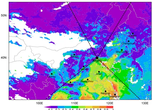
Fig. 1.Sampling location (116.30◦E, 39.99◦N) on a regional map superimposed with spatial distribution of annual mean fine aerosol optical depth (AOD) retrieved from MODIS satellite remote sensing in 2009. Dashed lines define four regions based on the trajectory clustering results discussed in Sect. 4.2 (seen in the text). Also shown are several major cities around Beijing.

burning, secondary sulfate, motor vehicles, secondary ni-trate, and road dust, with emphasis on coal combustion in winter and secondary aerosols in summer. Xie et al. (2008) conducted PMF analyses of PM10 (instead of PM2.5)

col-lected in Beijing in 10 days each in January, April, July, and October 2004 by using chemical data on metal elements, ions, and OC/EC as input data. Seven main sources were identified, including urban fugitive dust, crustal soil, coal combustion, secondary sulfate, secondary nitrate, biomass burning with municipal incineration, and vehicle emissions. All these studies were limited to a particular season and based on selected PM species.

To attain a better understanding of the chemical charac-teristics and sources of fine aerosols on a seasonal basis, we conducted a delicate investigation in Beijing. We continu-ously collected daily PM2.5samples at an urban site for four

months, each of which in the respective seasons (i.e., spring, summer, autumn and winter). The samples were subjected to chemical measurements of various aerosol compositions as a whole, such as a suite of crustal and anthropogenic el-ements, major water-soluble ions, and OC/EC. Furthermore, we identified and apportioned the main sources to PM2.5by

employing chemical mass closure construction and the PMF model in conjunction with trajectory cluster and potential source contribution function analyses according to the hybrid single-particle Lagrangian integrated trajectory (HYSPLIT) model. This study will elucidate the source profile of PM2.5

in different seasons and the relative contribution from each

source in the complex urban airshed in Beijing and provide vital information in formulating the future air management framework to address the current alarming level of PM pol-lution in China which has been affecting the air quality on a vast regional scale.

2 Methodology

2.1 Sample and chemical analysis

2.1.1 Sampling site

Beijing is located on the northern edge of the North China Plain, surrounded by the Yanshan Mountains in the west, north, and northeast (Fig. 1). According to the spatial dis-tribution of fine AOD ranging from 0.0 to 1.0 that has been retrieved from Moderate-resolution Imaging Spectrometer (MODIS) sensors on board Terra and Aqua satellites (Fig. 1), Beijing is one of the PM2.5 hot spots in China. The four

(4)

2.5

roof of the Science Building in Peking University (116.30◦_E, 39.99◦_{N) 26 m a.g.l. (above ground level). A few field} ex-perimental campaigns have been conducted at this urban site (He et al., 2010; Guo et al., 2012). This site is located within the educational, commercial, and residential districts, and no main pollution sources exist nearby. Thus, the observations could be typical of the general urban pollution in Beijing. 2.1.2 Sample collection

Daily PM2.5samples were collected in April, July, and

Octo-ber 2009 and January 2010, representing spring, summer, au-tumn, and winter, respectively. Two collocated aerosol sam-plers (frmOMNITM, BGI, USA) were used to collect PM2.5

samples from 10:00 to 10:00 LT the next day simultane-ously. The two substrates used in each sampler were 47 mm quartz filter (Whatman QM/A, England) and Teflon filter (pore size = 2 µm; Whatman PTFE, England). The flow rate was set at 5 L min−1. The quartz filters were baked at 800◦C for 3 h before use. The filter samples were stored at−18◦C until pretreatment.

2.1.3 Gravimetric weighing

Before and after each sampling, the PTFE filters were con-ditioned at 22◦_C_±₁◦_{C in relative humidity of 35 %}_±_{2 %} for 24 h and then weighed in a weighing room by using an electronic balance with a detection limit of 1 µg (Sartorius, G¨ottingen, Germany). The corresponding PM2.5mass

con-centration of each filter was equal to the weight difference before and after sampling divided by the sampled air volume. 2.1.4 Chemical analysis of trace elements and

water-soluble ions

Prior to extraction and digestion, each aerosol-laden PTFE membrane filter was cut into two equal halves with ceramic scissors. One half was subjected to Milli-Q water extrac-tion for ionic measurement and the other half to acid di-gestion for elemental measurement. For the acid didi-gestion, the polypropylene support O-ring on half of each PTFE filter sample was carefully removed with a ceramic knife from contamination. The filter samples were digested with an acid mixture (5 mL HNO3+2 mL HF) by using an

ultra-high throughout microwave digestion system (MARSXpress, CEM, Matthews, NC). A blank reagent and two filter blanks were prepared in each run following the same procedure used for the samples. All the acids used in this study were of ultra-pure grade (Merck, Germany). The detailed diges-tion method has been published elsewhere (Hsu et al., 2008). Another half of all filter samples were used for extrac-tion with 20 mL Milli-Q purified water (specific resistiv-ity = 18.2 Mcm−1; Millipore, Massachusetts, USA) for 1 h. The detailed extraction procedures have been described in Hsu et al. (2007, 2010a).

Ionic species (Na+ _{, NH}4+_{, K}+ _{, Mg}2+ _{, Ca}2+ _{, F}−_, Cl−_{, SO}2−

4 and NO

−

3) in the leachate were analyzed through

a Dionex model ICS-90 (for anions) and ICS-1500 (for cations) ion chromatograph equipped with a conductivity de-tector (ASRS-ULTRA). Trace elements in the digestion so-lutions, including Al, Fe, Na, Mg, K, Ca, Ba, Ti, Mn, Co, Ni, Cu, Zn, Mo, Cd, Sn, Sr, Sb, Pb, Tl, Ge, Cs, Ga, V, Cr, As, Se, and Rb, were analyzed by inductively coupled plasma–mass spectrometry (ICP–MS). Quality assurance and control of the ICP–MS was guaranteed by the analysis of a certified ref-erence standard, NIST SRM-1648 (urban particulates). The resulting recoveries fell within±10 % of the certified values for most elements, except for Se, As, Cs, Sb, and Rb (±15 %) (Hsu et al., 2009, 2010a).

2.1.5 OC and EC measurements

A punch of 0.526 cm2 from each quartz filter was heated stepwise by a thermal/optical carbon analyzer (DRI 2001, Atmoslytic, US) in a pure helium atmosphere at 140◦_C (OC1), 280◦_{C (OC2), 480}◦_{C (OC3), and 580}◦_{C (OC4),} and then in 2 % O2/98 % He atmosphere at 580◦C

(EC1), 740◦C (EC2), and 840◦C (EC3) to convert any particulate carbon on the filter to CO2. After

cat-alyzed by MnO2, CO2 was reduced to CH4, which was

then directly measured. Mass concentrations of OC and EC were obtained according to the IMPROVE protocol (Chow et al., 2007), OC = OC1+OC2+OC3+OC4+OP; EC = EC1+EC2+EC3-OP, where OP is the optical py-rolyzed OC. Detailed descriptions can be found in Zhang et al. (2012a).

2.2 Data analysis methods

2.2.1 Chemical mass closure

In this study, we constructed chemical mass closure (CMC) on a seasonal basis by considering mineral dust, SO2₄−, NO−₃, NH+₄, EC, particulate organic matter (POM), chloride salt (instead of sea salt; reason given below), trace element oxide (TEO), and biomass burning-derived K+. SO2₄−, NO−₃, and NH+₄ can be regarded as the secondary inorganic aerosols.

The aluminosilicate (i.e., soil, dust, or mineral) component is often estimated through the following formula (Malm et al., 1994; Chow et al., 1994), which includes Si.

[Mineral] =2.20 Al+2.49 Si+1.63 Ca+2.42 Fe+1.94 Ti

[Mineral] =1.89 Al+2.14 Si+1.40 Ca+1.43 Fe However, Si is volatilized as SiF4 in the acid digestion of

(5)

therein). Accordingly, we adopted a straightforward method conventionally used in estimating dust aerosols from Al:

[Mineral] =Al/0.07,

where 0.07 is the average Al content (7 %) reported by Zhang et al. (2003b). A similar estimation has been applied previ-ously (Ho et al., 2006; Hsu et al., 2010b).

In estimating POM, we adopted a factor of 1.6 in con-verting OC to POM (Viidanoja et al., 2002), whereas a wide range of 1.4–2.2 has been utilized in previous investigations (Turpin and Lim, 2001; Andreae et al., 2008). The main de-terminants in selecting a conversion factor are the origin and age of the organic aerosols. The factor of 1.6 was employed in this study because the latest result shows a OM/OC ra-tio averaged at 1.59±0.18 in PM2.5over China (Xing et al.,

2013). This factor was used for the PM2.5of Beijing by Dan

et al. (2004), who also observed a similar seasonality for EC and OC and a OC/EC ratio (2–3) close to our results.

Sea salt is usually calculated as [Sea salt] = 1.82×Cl− or = 2.54 Na+. Given that Beijing is about 150 km away from East China’s coastal oceans (i.e., Bohai Sea), sea spray-generated sea salt particles are not readily transported and are therefore insignificant to fine aerosols in Beijing. Nev-ertheless, dust blowing from Northern and Northwestern China is often associated with NaCl and Na2SO4from salt

lake sediments and saline soils (Zhang et al., 2009a). On the other hand, Cl−_{may be essentially contributed by coal} combustion in Beijing, particularly in winter (Yao et al., 2002). Thus, we considered chloride salt, instead of sea salt, as an individual component of PM2.5 aerosols in

Bei-jing: [Cl salt] = [Cl−_]₊_[Na+_]₊_[ss-Mg2+_{]. By considering} chloride depletion in sea salt particles within the marine boundary layer because of the heterogeneous reaction, Hsu et al. (2010a) successfully evaluated such formula.

Following Landis et al. (2001), we estimated the contribu-tion of heavy metals as metal oxides by employing the fol-lowing equation:

TEO=1.3×[0.5×(Sr+Ba+Mn+Co+Rb+Ni+V)

+1.0×(Cu+Zn+Mo+Cd+Sn+Sb+Tl

+Pb+As+Se+Ge+Cs+Ga)].

The enrichment factor (EF) of a given element (E) was cal-culated by using the formula EF = (E/Al)Aerosol/(E/Al)Crust

(Hsu et al., 2010a), where (E/Al)Aerosolis the ratio of the

el-ement to the Al mass in aerosols and (E/Al)Crustis the ratio

in the average crust (Taylor, 1964). The result of the EF is shown in Fig. S1 (Supplement). Elements with EFs of≤1.0, such as Cr and Y, were not considered, as they are of exclu-sive crustal origin. Elements with EFs between 1 and 5 were multiplied by a factor of 0.5, as they are possibly originated from two sources (i.e., anthropogenic and crustal sources). Elements with EFs≥5.0 were multiplied by unity, as they are dominated by anthropogenic origins. Furthermore, the multiplicative factor was set at 1.3 so that metal abundance

could be converted to oxide abundance, similar to those used by Landis et al. (2001). We also considered biomass burning-derived K+_(K

BB) as an individual component, although KBB

salt may exist in the chemical forms of KCl and K2SO4

(P´osfai et al., 2004), where both Cl−and SO2₄−have already been considered in other components.

2.2.2 PMF model

PMF is an effective source apportionment receptor model that does not require the source profiles prior to analysis and has no limitation on source numbers (Hopke, 2003; Shen et al., 2010). The principles of PMF can be found elsewhere in detail (Han et al., 2006; Song et al., 2006; Yu et al., 2013). In the present study, PMF 3.0 was employed with the inclusion of 34 chemical species in the model computation: PM2.5, Al,

Fe, Na, Mg, K, Ca, Ba, Ti, Mn, Co, Ni, Cu, Zn, Mo, Cd, Sn, Sb, Pb, V, Cr, As, Se, Rb, Na+_{, NH}+

4, K+, Mg2+, Ca2+, Cl−,

SO2₄−, NO−₃, OC, and EC. Six physically realistic sources were identified.

2.2.3 Air mass back trajectory cluster

We calculated 48 h air mass back trajectories arriving at the sampling site (116.30◦_{E, 39.99}◦_{N) during our sampling} pe-riod by using the National Oceanic and Atmospheric Admin-istration (NOAA) HYSPLIT-4 model with a 1◦_×₁◦_latitude– longitude grid and the final meteorological database. The six-hourly final archive data were generated from the National Center for Environmental Prediction’s Global Data Assimi-lation System (GDAS) wind field reanalysis. GDAS uses a spectral medium-range forecast model. More details about the HYSPLIT model can be found at http://www.arl.noaa. gov/ready/open/hysplit4.html (NOAA Air Resources Labo-ratory). The model was run four times per day at starting times of 04:00, 10:00, 16:00, and 22:00 UTC (12:00, 18:00, 00:00, and 06:00 LT – local time, respectively). The arrival level was set at 100 m a.g.l. The method used in trajectory clustering was based on the GIS-based software TrajStat (http://www.meteothinker.com/TrajStatProduct.aspx).

2.2.4 Potential source contribution function

The potential source contribution function (PSCF) is a method for identifying regional sources based on the HYS-PLIT model. The zone of concern is divided intoi×j small equal grid cells. The PSCF value in theij-th cell is defined as

(6)

2.5

Table 1.Statistical summary showing the means (with one standard deviation) and ranges of atmospheric concentrations for PM₂_.₅(in unit

µg m−3) and selected species (in unit ng m−3) in the entire sampling (annual) and four-season (months) periods.

Species Annual Spring Summer Autumn Winter

PM₂.5 135±63 126±59 138±48 135±55 139±86

39–355 39–280 41–226 45–251 48–355

SO2₄− 13.6±12.4 14.7±11.5 23.5±14.5 7.9±7.4 8.5±8.6

0.9–52.8 2.3–52.8 2.5–52.0 0.9–25.7 1.3–34.4

NO−₃ 11.3±10.8 15.5±13.7 11.8±8.2 10.7±11.0 7.3±8.1

0.3–63.8 1.3–63.8 1.8–31.5 0.3–34.7 1.6–35.5

NH+₄ 6.9±7.1 7.5±8.1 11.0±6.9 4.7±5.8 4.5±5.7

0.1–39.1 0.6–39.1 0.5–23.9 0.1–17.7 0.3–23.3

Cl− _1.42_±_2.18 _0.72_±_0.81 _0.30_±_0.56 _1.12_±_0.98 _3.52_±_3.32

0.03–10.34 0.04–3.74 0.03–3.06 0.09–3.71 0.19–10.34

Na+ 0.46±0.55 0.31±0.18 0.17±0.09 0.30±0.22 1.08±0.80

0.04–2.82 0.08–0.94 0.04–0.42 0.05–1.06 0.11–2.82

K+ 0.92±0.75 1.08±0.71 0.66±0.47 1.13±0.90 0.81±0.77

0.03–3.66 0.14–3.14 0.20–2.47 0.03–3.66 0.05–2.53

Mg2+ 0.16±0.13 0.24±0.20 0.07±0.03 0.16±0.07 0.18±0.09

0.02–1.04 0.03–1.04 0.02–0.16 0.06–0.31 0.06–0.45

Ca2+ 1.6±1.5 2.6±2.2 0.6±0.3 1.7±1.0 1.5±0.9

0.2–11.3 0.2–11.3 0.2–1.7 0.5–4.2 0.5–4.0

Al 1.8±1.5 2.5±1.7 0.7±0.4 2.0±1.4 2.1±1.5

0.1–6.9 0.3–6.6 0.1–2.0 0.3–6.7 0.7–6.9

OC 16.9±10.0 13.7±4.4 11.1±1.8 17.8±5.6 24.9±15.6

5.9–58.6 5.9–23.7 7.4–16.6 7.5–26.2 8.5–58.6

EC 5.0±4.4 2.8±1.1 4.2±1.2 5.3±2.8 7.5±7.4

0.6–28.1 0.6–5.8 1.5–6.8 1.3–12.1 1.2–28.1

wij =

   

  

1.00 80< nij 0.70 20< nij ≤80 0.42 10< nij ≤20 0.05nij ≤10

   

  

.

The study domain was in the range of 30–60◦N, 75–130◦E. The resolution was 0.5◦×0.5◦.

3 Results

3.1 Annual average

Table 1 provides a statistical summary of the obtained data on atmospheric concentrations for PM2.5, Al (a tracer of

alu-minosilicate dust), water-soluble ions, OC, and EC during the sampling period. The annual mean PM2.5concentration

reached 135±63 µg m−3. This mean value is nearly three times higher than that (35 µg m−3) of the interim target-1 standard for annual mean PM2.5recommended by the WHO.

The level of PM2.5 in Beijing is much higher than other

mega-cities around the world. In comparison with that of do-mestic cities, PM2.5seems to display a spatial tendency,

in-creasing northward and dein-creasing southward (Zhang et al.,

2012b). Such a spatial pattern may be related to the low rain-fall and high dust in northern China (Qian et al., 2002; Qian and Lin, 2005). According to Wang et al. (2008), PM2.5

con-centrations in winter were much higher than in summer in 2001 to 2002. However, such a trend seemed to be reversed in 2005 to 2006, with rather higher concentrations in summer.

For the ionic concentrations, SO2₄− ranked the high-est among the water-soluble ions analyzed, with an annual mean of 13.6±12.4 µg m−3_, _followed _by

NO−₃ (11.3±10.8 µg m−3_), _NH+

4 (6.9±7.1 µg m3),

(7)

S S A W 0

100 200

Conc

ent

rat

ion

μ

g/

m

3

PM_2.5

S S A W

0 20 40 SO₄

2-S S A W

0 15

30 _NO

3

-S S A W

0 10 20

Conc

ent

rat

ion

μ

g/

m

3 NH4

+

S S A W

0 1 2 Na+

S S A W

0.00 0.25

0.50 _Mg2+

S S A W

0.0 1.5 3.0

Conc

ent

rat

ion

μ

g/

m

3 K

+

S S A W

0.0 2.5 5.0

Ca2+

S S A W

0 4 8 Cl

-S S A W

0 23 46

Conc

ent

rat

ion

μ

g/

m

3 OC

S S A W

0 8 16 EC

S S A W

0.0 2.5 5.0

Al

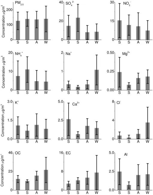
Fig. 2.Seasonal variations of PM₂_.₅mass concentration and associated species, including SO2₄−, NO−₃, NH+₄, Na+, Mg2+, K+, Ca2+, Cl−, OC, EC, and Al concentrations. Shown here are the mean and one standard deviation for each bar.

regional sites across China (16.1±5.2 µg m−3 _{for OC}

and 3.6±0.93 µg m3 for EC) by Zhang et al. (2008), who extensively measured carbonaceous aerosols around China; however, such concentrations are approximately half of those observed at urban sites (33.1±9.6 µg m−3_{for OC and}

11.2±2.0 µg m−3_{for EC) by Zhang et al. (2008).}

3.2 Seasonality

As illustrated in Fig. 2, the seasonality of PM2.5 and these

primary species were characterized by distinctive features. The seasonality of PM2.5 concentration was not very

evi-dent and typical, with nearly equal concentrations of around 140 µg m−3 _{in summer, autumn, and winter and a relative}

minimum (∼125 µg m−3_{) in spring. The minimum}

concen-tration typically occurs in summer because precipitation in Beijing is usually concentrated at that period (Fig. S2, Sup-plement). However, this is not the case, because the max-imum concentrations of secondary sulfate and ammonium were observed in summer, arising from strong photochem-istry and accounting for a large proportion (∼25 %) of PM2.5

(8)

2.5

the photochemical effect might overwhelm the precipitation scavenging effect for fine aerosol pollutants.

In contrast to PM2.5, sulfate and ammonium revealed a

typical seasonality with higher concentrations in spring and summer and lower concentrations in autumn and winter, consistent with the seasonal variability of AOT (Xia et al., 2006). The summertime maximum concentrations of sulfate and ammonium were 24 and 12 µg m−3, respectively, which were higher than those in Beijing before 2003 (∼15 and

≤10 µg m−3_{, respectively) (He et al., 2001; Duan et al.,}

2006; Wang et al., 2005) but rather comparable to those ob-served in the last few years (Okuda et al., 2011; Song et al., 2012). By contrast, the wintertime concentration of sulfate (8.5 µg/m3)was significantly reduced compared with ear-lier literature data (He et al., 2001; Hu et al., 2002, Wang et al., 2005). The decrease in wintertime sulfate concentra-tion seemed to result from the effective control of SO2

emis-sions over China in the recent years (Itahashi et al., 2012), particularly from coal combustion (Hao et al., 2005). High summertime sulfate concentration is ascribed to enhanced photochemistry during summer, and relatively high humid-ity accelerates the conversion rate of SO2to the particulate

form (Yao et al., 2003). However, the precursor SO2

con-centrations are much higher in winter (Fig. S3, Supplement) because of higher emission at that time (Zhang et al., 2009b). One might further conclude that in Beijing, photochemistry plays a more vital role in the sulfate aerosol formation and variability than the change in precursor SO2emission as well

as rain scavenging process. In the present study, artificial biases, particularly of nitrate and ammonium, possibly oc-curred during sampling because no denuder and/or back-up filter was used to trap ammonia and nitric acid (Pathak et al., 2004). The maximum concentration (15.5 µg m−3_{) of}

ni-trate was observed in spring rather than summer, which was different from that of sulfate (Wang et al., 2008). This ob-servation may be ascribed to the volatility of ammonium ni-trate, which is one of the main chemical forms of nitrate as-sociations revealed by the ionic relationships. Thus, ammo-nium nitrate could evaporate at relatively high temperature. Besides, there are distinct emission sources for their respec-tive precursor gases, SO2and NOx. The minimum

concen-tration of nitrate was observed in winter. Nitrate levels could be a function of various factors in terms of emissions, such as vehicular exhaust, coal combustion, and biomass burning, and complex chemical processes with respect to photochem-istry, heterogeneous reaction, renoxification, and gas-aerosol equilibrium. The overall trend of NOxemission in China is

increasing primarily due to persistently increasing energy de-mand for industrial development and transportation, though control measures for NOxemissions have been implemented

in coal-fired power plants (Zhao et al., 2013).

Crustally derived ions and elements, such as Mg2+, Ca2+, and Al, waxed in the spring and waned in the summer, fol-lowed by significant increases toward autumn and winter. Such levels of seasonal mean concentrations and seasonality

are consistent with those observed in previous studies (Duan et al., 2006; Wang et al., 2005), which are related to dust storms and anthropogenic and fugitive dust. The seasonal concentrations of Na+and Cl−peaked in winter, consistent with Hu et al. (2002) and Wang et al. (2005). The seasonality of Mg2+was distinguishable from that of Na+, demonstrat-ing the difference in their dominant sources. K+ had rela-tively higher concentrations in both spring and autumn than in summer and winter, which was closely associated with the agricultural burning around Beijing (Zheng et al., 2005). Such seasonality was also found by some previous studies (He et al., 2001; Zheng et al., 2005), but distinct from other previous studies, in which winter often had the highest con-centration (Duan et al., 2006; Wang et al., 2005). Specifically, the highest levoglucosan, which is suggested to serve as an excellent tracer of biomass burning pollutants relative to K+_, has been measured in autumn (He et al., 2006), although no spring sample was measured in that study.

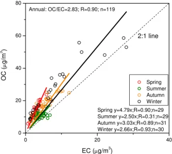
Both OC and EC had similar seasonal patterns of wax-ing in winter and wanwax-ing in sprwax-ing (for EC) or summer (for OC). Zhang et al. (2008) observed a persistently common seasonality for both OC and EC at 18 background, regional, and urban stations in China, i.e., a maximum in winter and a minimum in summer. The seasonality may be governed by the variability in emission strengths and meteorology. For in-stance, lower-molecular weight semi-volatile organic com-pounds are mostly in gaseous phase at high temperature in summer (Yassaa et al., 2001). The OC/EC mass ratio 2.0 in-dicates the presence of secondary organic matter (Chow et al., 1996). In this work, the OC/EC ratios mostly fell within the range of 2–5, with mean ratios of 4.8, 2.5, 3.0, and 2.7 in spring, summer, autumn, and winter, respectively (Fig. 3). These figures are very similar to those observed in previous studies (Duan et al., 2006; Zhang et al., 2008), which sug-gests the relative domination of secondary organic aerosols in spring but of primary sources in other seasons (Zhang et al., 2008). Another reason for the relatively higher spring-time OC/EC mass ratio may be the open biomass burning source, consistent with higher K+in the spring (Fig. 2), as the aerosols from open biomass burning are generally char-acterized by elevated OC/EC ratios (Cao et al., 2007).

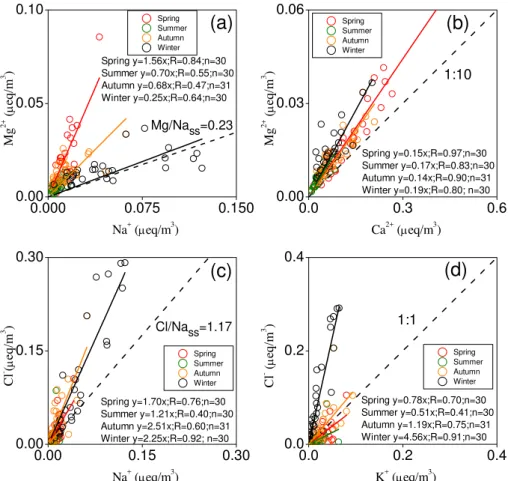
3.3 Stoichiometric analyses of cations and anions

Note that equivalent concentrations (µeq m−3_{) are used}

throughout this section. Figure 4 shows the scatter plots of (a) Mg2+ _{vs. Na}+_{, (b) Mg}2+ _{vs. Ca}2+_{, (c) Cl}− _{vs. Na}+_, and (d) Cl− _{vs. K}+_{. Figure 5 shows the scatter plots of} (a) total cations vs. total anions, (b) NH+₄ vs. SO2₄−, (c) NH+₄ vs. [SO2₄−+NO−₃], (d) [NH+₄ +Ca2+_{] vs. [SO}2−

4 +NO

−

3],

(9)

Spring Summer Autumn Winter

0 20 40

0 20 40 60 80

Spring y=4.79x;R=0.90;n=29 Summer y=2.50x;R=0.31;n=29 Autumn y=3.03x;R=0.89;n=31 Winter y=2.66x;R=0.93;n=30

2:1 line

EC (μg/m3)

OC

(

μ

g/

m

3 )

Annual: OC/EC=2.83; R=0.90; n=119

Fig. 3.Scatter plot showing the correlation between OC (yaxis)

and EC (xaxis) in PM₂.5collected from Beijing. Different symbols

denote the four seasons. Linear regression equations are given in the annual and seasonal cases.

as the tracer of sea salt: Ex-Cl−_{= Cl}−₋_[Na+_]_×_1.17, where 1.17 is the typical Cl−_/Na+ _{equivalent ratio of} average seawater (Chester, 1990). If the resulting Ex-Cl− is negative, then no Cl− _{excess exists. In other words, Cl}− is totally contributed by sea salt and is even depleted by heterogeneous reactions. Nevertheless, total Na+ _{does not} necessarily originate from sea salt alone, but could partially come from dust. The resultant biases are hence likely insignificant.

Figure 4a illustrates that Mg2+ mostly comes from non-sea salt sources, except in wintertime, because the regres-sion slopes that represent the Mg2+/Na+ ratios (1.56, 0.70, 0.68, and 0.25 for spring, summer, autumn, and winter, re-spectively) are clearly deviated from the ratio (0.23) of av-erage seawater (Chester, 1990). Instead, the dominant source of Mg2+_{is mineral dust, mainly carbonate minerals (Li et al.,} 2007), as reflected by the good correlations (0.97, 0.83, 0.90, and 0.80 for spring, summer, autumn, and winter, respec-tively) between Mg2+ _{and Ca}2+ _{(Fig. 4b). Similarly, most} Cl−_/Na+_{ratios (1.70, 1.21, 2.51, and 2.25 for spring,} sum-mer, autumn, and winter, respectively) in PM2.5 are larger

than the mean ratio (1.17) of seawater, except the summer-time samples (Fig. 4c). This difference indicates the domi-nance of the non-sea salt sources, of which the most likely contributor of Cl−is coal combustion (Yao et al., 2002), par-ticularly in winter when Cl− and SO2are maximal (Figs. 2

and S2, Supplement). In summer, air masses are dominated by the southerly monsoon from Bohai (as supported by the trajectories below), leading to a mean Cl−/Na+ ratio close to that of average seawater. Moreover, the correlations be-tween K+ _{and Cl}− _{largely varied with the seasons, with}

better correlation and higher ratios in autumn and winter and moderate correlations and lower ratios (less than unity) in summer and spring (Fig. 4d). Thus, the results suggested that K+ was not present in chemical form KCl at high temper-ature, but as K2SO4 (P´osfai et al., 2004). By contrast, low

temperature in winter may favor the presence of KCl. Furthermore, the ratio of total cation concentration to to-tal anion concentration is averaged at near unity throughout the year (Fig. 5a), which indicates excellent charge balance in PM2.5 and high data quality. Figure 5b shows good

cor-relations between NH+₄ and SO2₄− for the annual data set, with ratios (represented by the slope of the linear regression line) between 1.25 and 1.77 (all higher than unity). These good correlations reveal the dominance of (NH4)2SO4

(Ian-niello et al., 2011), rather than NH4HSO4and the possible

full neutralization of SO2₄− by NH+₄ throughout the year. We further considered the combination of NO−₃ and SO2₄− in this charge balance analysis (Fig. 5c). The resulting NH+₄ to [SO2₄−+NO−₃] ratios ranged from 0.83 to 0.94 (all lower than unity), which demonstrates the presence of NH4NO3

in the fine-mode aerosols. Moreover, ratios lower than unity suggest that nitrate may be present in other chemical forms than NH4NO3. Heterogeneous reactions between NOx(and

its products, such as HNO3 and N2O5)and dust carbonate

are often observed in northern China (Li and Shao, 2009). Accordingly, we examined the correlations of [NH+₄ +Ca2+] vs. [SO2₄−+NO−₃] (Fig. 5d) and of [NH₄++Ca2+₊_Mg2+_] vs. [SO2₄−+NO−₃] (Fig. 5e), given that the good correla-tions between Mg2+_{and Ca}2+_{suggest the possible existence} of water-soluble Mg in reacted carbonate dust. These ions are strongly correlated throughout the year, with high co-efficients (all 0.99 or higher) and slopes of regression lines around unity. These correlations indicate that nitrate is partly present in Ca(NO3)2 and Mg(NO3)2, not just in NH4NO3.

We assumed that fine-mode sulfate is exclusively associated with ammonium and that Na+_{is present only in the} associ-ated NaCl. However, these assumptions may not always be true because Na2SO4is observed in dust particles from dried

lakes in northern China (Zhang et al., 2009a) and NaCl could react with nitric acid to form NaNO3via heterogeneous

re-action (Hsu et al., 2007). Therefore, based on the afore-mentioned equivalent interrelationships and assumptions, we quantitatively estimated that the former two chemical forms (Ca(NO3)2and Mg(NO3)2) represent∼20 % of the total

ni-trate and that NH4NO3is the dominant association

account-ing for the remainaccount-ing∼80 %. The elevated Cl−/Na+ ratio (>1.17) shows that excessive Cl− seemed to be attributed to coal combustion rather than sea salt particles from dried salt lake sediment. The addition of excessive Cl− (Fig. 5f) insignificantly changed the correlations of positive and neg-ative charges. Nevertheless, we noted that in wintertime, the equivalent ratio improved from 1.10 to 1.00, which indicates the presence of chloride salts such as KCl, CaCl2, and MgCl2

(10)

2.5

0.000 0.075 0.150

0.00 0.05 0.10

0.00 0.15 0.30

0.0 0.3 0.6

0.00 0.03 0.06

0.0 0.2 0.4

0.0 0.2 0.4 Spring

Summer Autumn Winter

Mg

2+ (

μ

eq

/m

3 )

Na+ (μeq/m3)

Mg/Na_ss=0.23

(a)

(c)

Spring y=1.70x;R=0.76;n=30 Summer y=1.21x;R=0.40;n=30 Autumn y=2.51x;R=0.60;n=31 Winter y=2.25x;R=0.92; n=30

Cl

- (μ

eq

/m

3 )

Na+ (μeq/m3)

Cl/Na_ss=1.17

(b)

Spring y=0.15x;R=0.97;n=30 Summer y=0.17x;R=0.83;n=30 Autumn y=0.14x;R=0.90;n=31 Winter y=0.19x;R=0.80; n=30

Mg

2+ (

μ

eq

/m

3 )

Ca2+ (μeq/m3)

1:10

(d)

1:1

Cl

- (

μ

eq

/m

3 )

K+ (μeq/m3)

Fig. 4.Correlations between certain cations and anions:(a)Mg2+versus Na+,(b)Mg2+versus Ca2+,(c)Cl−versus Na+, and(d)Cl−

versus K+. Four seasons are considered and represented by different color symbols. Linear regression equations are also given. In(a)and(c),

the dashed lines indicate the Mg/Na and Cl/Na equivalent concentration ratios in seawater (sea salt), respectively.

2011). KCl may have originated from biomass burning, and CaCl2and MgCl2could have been formed through

heteroge-neous reactions between the dust carbonate and HCl emitted from coal combustion.

3.4 Chemical mass closure

By employing the methods in Sect. 2.6, we constructed the CMC of PM2.5 in Beijing on a seasonal and annual

ba-sis. The reconstructed PM2.5mass concentrations were

com-pared with the gravimetric PM2.5 mass concentrations, as

shown in Fig. 6, which shows a good correlation with one another in each season and throughout the year. However, the ratios seasonally changed, with higher ratios of 0.82 in spring and 0.75 in winter and lower ratios of 0.59 in summer and 0.68 in autumn. The proportions of all specific compo-nents in PM2.5together with the unidentified constituents as

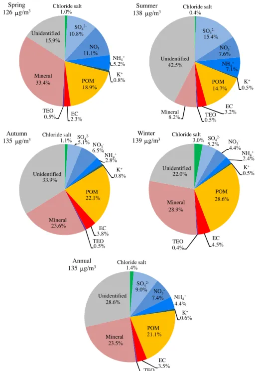
a whole are schematically illustrated by five pie charts for the four seasonal and annual cases (Fig. 7). Overall, the ma-jor components are secondary inorganic aerosols (combina-tion of sulfate, nitrate, and ammonium), mineral dust, and POM, which account for each∼20 %, albeit with seasonal

variations. The minor components include EC, chloride salt, potassium salt, and TEO, each of which represents less than 5 %. Specifically, the proportions of mineral dust are max-imal (33.4 %) in spring, minmax-imal (only 8.2 %) in summer, and intermediate (23.6 and 28.9 %) in the other two sea-sons, consistent with the tendency of seasonal Al concen-trations. The totals of secondary inorganic species (SO2₄−, NO−₃, and NH+₄) have the largest proportion (27 to 30 %) in spring and summer and a minimal percentage (<15 %) in autumn and winter. However, sulfate peaks were noted in summer (15.4 %), whereas nitrate peaks were observed in spring (11.1 %). Ammonium decreased from around 5 to 7 % in spring and summer to half (2 to 3 %) in autumn and winter. The POM fractions largely varied as follows: sum-mer (14.7 %)<spring (18.9 %)<autumn (22.1 %)<winter (28.6 %). EC and chloride salt exhibited the largest propor-tions (5.2 and 3.3 %, respectively) in winter. Potassium salt and TEO had slightly higher proportions in spring and au-tumn than in summer and winter.

Both the primary and secondary components of PM2.5in

(11)

0.0 0.5 1.0 1.5 2.0 2.5 0.0 0.5 1.0 1.5 2.0 2.5

0.0 0.5 1.0 1.5 2.0 2.5 0.0 0.5 1.0 1.5 2.0 2.5 Spring Summer Autumn Winter Spring y=1.02x;R=0.997;n=30 Summer y=0.96x;R=0.997;n=30 Autumn y=1.02x;R=0.998;n=31 Winter y=0.97x;R=0.999;n=30 Σ canions ( μ eq/m 3 )

Σ anions (μeq/m3)

(a)

1:1 line Spring Summer Autumn Winter Spring y=1.52x;R=0.95;n=30 Summer y=1.25x;R=0.97;n=30 Autumn y=1.77x;R=0.98;n=31 Winter y=1.59x;R=0.99;n=30

(b)

1:1 line NH 4 + ( μ eq /m 3 )

SO₄2- (μeq/m3)

Spring Summer Autumn Winter Spring y=0.83x;R=0.96;n=30 Summer y=0.90x;R=0.996;n=30 Autumn y=0.87x;R=0.99;n=31 Winter y=0.94x;R=0.996;n=30

(c)

1:1 line NH 4 + ( μ eq/ m 3 )

SO₄2- + NO₃-(μeq/m3)

(d)

1:1 line NH 4

+ + C

a

2+ (

μ

eq/m

3 )

(e)

1:1 line NH 4

+ + C

a

2+ +M

g 2+ ( μ eq /m 3 )

(f)

1:1 line NH 4 + + C a

2+ +Mg 2+ + K

+ (

μ

eq/

m

3 )

SO₄2- + NO₃-+Ex-Cl-(μeq/m3)

Fig. 5.Same as Fig. 4, but for(a)total cations versus total anions,(b)NH+₄ versus SO2₄−,(c)NH+₄ versus [SO2₄−+NO−₃],(d)[NH+₄ +Ca2+_]

versus [SO2₄−+NO−₃],(e)[NH+₄ +Ca2++Mg2+] versus [SO2₄−+NO−₃], and(f)[NH+₄+Ca2++Mg2+] versus [SO2₄−+NO−₃ +

Ex-Cl−]. The detailed definition of Ex-Cl−(Excessive-Cl−) can be found in the text. The 1 : 1 lines are given for comparison.

2006). In general, given that the seasonal variability in PM2.5

mass concentrations is relatively small, temporal trends in the proportions of each component of PM2.5 resemble the

atmospheric concentrations of their corresponding chemical species. The likely factors for such seasonality are partially addressed in Sect. 3.2 and discussed in detail in the following two sections.

On average, the unidentified components reached 28.6 % of the total PM2.5. They also showed seasonal variability,

(12)

2.5

0 100 200 300 400

Spring

Summer

Autumn Winter

y=0.79x R=0.94 y=0.57x R=0.95 y=0.65x R=0.92

1:1 l ine

Gravimetric (μg/m3

)

R

e

constructed

(

μ

g/m

3 )

y=0.72x R=0.96 y=0.68x R=0.91 Annual

Fig. 6. Scatter plot showing the correlations between the PM₂_.₅ mass concentrations reconstructed from the chemical mass balance method and obtained from gravimetric measurement, which are pre-sented on a seasonal basis. Linear regression lines are shown with equations for the four-season period, along with the annual case.

Tsai and Kuo, 2005). The absorption likely led to positive bi-ases in PM2.5concentrations. Alternatively, such

uncertain-ties may be partly due to the volatilization of NH4NO3and

organic matter, particularly in summer and autumn during the storage of the weighted samples prior to extraction, which may have resulted in negative biases in the specific compo-nents. Another likely reason for the non-match of the recon-structed and gravimetric mass concentrations is the varying factors used in transferring a given analyzed species (e.g., OC and Al) to a certain component (e.g., POM and mineral soils) (Rees et al., 2004; Hsu et al., 2010a; Yan et al., 2012). For example, a few studies adopted a factor of only 1.4 for converting OC content to organic matter (Duan et al., 2006; Song et al., 2007; Guinot et al., 2007). Another study ob-tained a much higher POM/OC mean ratio over China (Xing et al., 2013) of up to 1.92±0.39 based on a mass balance method. If we adopt this higher ratio, the unidentified per-centage would be reduced by 3 %. In the present study, the EFcrust of Ca averages at 2.6, which shows its enrichment

relative to average crust composition. In Beijing, fine-mode Ca-rich dust is partly attributed to construction activities. Therefore, we may underestimate carbonate abundance in the mineral component estimated from Al concentration alone (Guinot et al., 2007). This may have resulted in the underes-timation (∼2 %) of the total mass reconstructed.

Table 2.Relative contributions from six identified sources of PM₂_.₅ in Beijing within the one-year and four-season periods.

Source Spring Summer Autumn Winter Annual

Soil dust 23 % 3 % 18 % 16 % 15 % Coal combustion 5 % 1 % 7 % 57 % 18 % Biomass burning 19 % 6 % 17 % 7 % 12 % Traffic and waste 5 % 4 % 4 % 2 % 4 % incineration emission

Industrial pollution 14 % 32 % 42 % 12 % 25 % SIA 34 % 54 % 13 % 6 % 26 %

4 Discussion

4.1 Source identification and apportionment

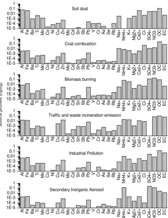
By utilizing the PMF model with the obtained full data set as input data, we identified six main sources: mineral dust, biomass burning, coal combustion, traffic emissions plus waste incineration, industrial pollution, and secondary in-organic aerosol. Table 2 summarizes the source apportion-ment results of the relative contributions from each identi-fied source to the PM2.5on both a seasonal and annual basis

in Beijing. These sources have average contributions of 15, 18, 12, 4, 25, and 26 % (Table 2). Figures 8 and 9 show the modeled source profiles and the time series of modeled con-centrations for each identified main source. Again, the rela-tive dominance of each identified source largely varies with changing seasons, which is roughly consistent with the CMC results. For mineral dust, only one of the six sources mostly dominated by nonvolatile substance, its proportions (e.g., an-nual mean∼20 %) and relative order in the four seasons are consistent with the CMC results, with the highest contribu-tion in spring, the lowest contribucontribu-tion in summer, and inter-mediate contribution in autumn and winter. This consistency indirectly verifies the reliability of the PMF results. The other five sources all appear to be related to high-temperature ac-tivities and/or photochemical processes and involved with volatile species. We then compared the contribution percent-ages of the secondary inorganic aerosol (SIA) with the CMC results as this source is also identified in the CMC analy-ses. Apparently, the percentages of SIA in the four seasons differ from those obtained by CMC in terms of the values (e.g., 6 to 54 % versus 14 to 33 % for SIA), although the seasonal trends are quite similar. Thus, CMC method only offers chemical characterization instead of source apportion-ment. The PMF model provides real information on sources of aerosol speciation.

(13)

1.0%

10.8%

11.1%

5.2%

0.8% 18.9%

2.3% 0.5%

33.4% 15.9%

Spring 126 g/m3

Unidentified Chloride salt

SO4

2-NO3

-NH4+

K+ POM

EC TEO Mineral

0.4%

15.4%

7.6%

7.1%

0.5% 14.7%

3.2% 0.5% 8.2%

42.5%

Summer 138 g/m3

SO4

2-NO3

-NH4+

K+ POM

EC TEO Mineral

1.1% _5.1%

6.5%

2.8%

0.8%

22.1%

3.8%

0.5% 23.6%

33.9%

Autumn 135 g/m3

Unidentified Chloride salt _SO

4

2-NO3

-NH4+

K+

POM

EC

TEO Mineral

3.0% 5.2%

4.4%

2.4%

0.5%

28.6%

4.5% 0.4%

28.9% 22.0%

Winter 139 g/m3

SO42- _NO

3

-NH4+

K+

POM

EC TEO

Mineral

1.4%

9.0% 7.4%

4.4%

0.6%

21.1%

3.5%

0.5% 23.5%

28.6%

Annual 135 g/m3

SO4 2-NO3

-NH4+

K+

POM

EC

TEO Mineral

μ μ

μ

Fig. 7.Pie-charts showing the constructed chemical mass closures for PM₂.5in Beijing:(a)spring;(b)summer;(c)autumn;(d)winter;

and(e)annual. The components include mineral dust, secondary aerosol ions (sulfate, nitrate, and ammonium), POM, EC, trace element

oxides (TEO), chloride salt, and biomass burning-derived potassium. Other than the identified components, unidentified fractions comprise

a significant portion of PM₂_.₅.

of high levels of OC (Watson and Chow, 2001). Thus, this source possibly mixes desert/loess dust, anthropogenic con-struction dust, fugitive dust, and resuspended road dust. Construction activities are prevalent in the urban cities of China, and no effective measures for dust control are imple-mented. Therefore, calcium is used as an indicator element

(14)

2.5

Al Fe Ba Ti Mn Co Ni Cu Zn Mo Cd Sn Sb Pb V Cr As Se Rb _Na+

NH

4+ K+

Mg2

+

Ca

2+ Cl

-SO

4=

NO

3- _OC _EC

1E-5 1E-4 1E-3 0.01 0.1 1 Source profiles ( μ g/ μ g) Soil dust

Al _Fe _Ba Ti _Mn _Co Ni Cu Zn Mo Cd Sn Sb Pb V Cr As Se Rb

Na+ NH 4+ K+ Mg2 + Ca2+ Cl-SO 4= NO

3- _OC _EC

1E-5 1E-4 1E-3 0.01 0.1 1 Coal combustion

Al _Fe _Ba Ti _Mn _Co Ni _Cu Zn Mo Cd Sn Sb Pb V Cr As Se Rb _Na+

NH

4+ K+

Mg2

+

Ca

2+ Cl

-SO 4= NO 3-OC EC 1E-5 1E-4 1E-3 0.01 0.1 1 Biomass burning

NH 4+ K+ Mg 2 + Ca2+ Cl-SO 4= NO

3- _OC _EC

1E-5 1E-4 1E-3 0.01 0.1 1

Traffic and waste incineration emission

NH 4+ K+ Mg2 + Ca2+ Cl-SO 4= NO

3- _OC _EC

1E-5 1E-4 1E-3 0.01 0.1 1 Industrial Pollution

Al _Fe _Ba Ti _Mn _Co Ni _Cu Zn Mo Cd Sn Sb Pb V Cr As Se Rb _Na+

NH

4+ K+

Mg2

+

Ca

2+ Cl

-SO 4= NO 3-OC EC 1E-5 1E-4 1E-3 0.01 0.1 1

Secondary Inorganic Aerosol

Fig. 8.Profiles of six sources identified from the PMF model, in-cluding soil dust, coal combustion, biomass burning, traffic and waste incineration emission, industrial pollution, and secondary in-organic aerosol (from the upper to the lower panels).

et al., 2008). Coal combustion is the predominant source of fine aerosols over China (Yao et al., 2009), which has re-sulted in severe air pollution problem not only locally, but also regionally and globally; for instance, it alone contributes more than 10 % (268 Mg) of the global anthropogenic mer-cury emission (2319 Mt) annually (Pirrone et al., 2010). Be-sides, coal fly ash could be one of the main contributors of aerosol Pb in China as they contain abundant Pb (Zhang et al., 2009c). Sodium has also been found to be enriched in fine particulates from coal combustion (Takuwa et al., 2006). Wang et al. (2008) and Zhang et al. (2009a) attributed the observed high Na and Cl to the presence of Na2SO4 and

NaCl that may be originated from dried lake salt sediment in Inner Mongolia, a non-local dust source. However, as dis-cussed, salt lake aerosols alone cannot account for such strik-ingly high Cl− in winter, which suggests that coal combus-tion is the most likely dominant source. Different investi-gations have obtained significantly different contributions of coal combustion to PM2.5in Beijing, which range from 7 to

19 %. Yao et al. (2009) concluded that the likely fraction ranges between 15 and 20 %. Nevertheless, previous studies have not considered that other main identified sources, such

as secondary inorganic and organic aerosols, have contribu-tions from coal combustion.

The third source, biomass burning, is characterized by high K (K+), which is an excellent tracer of biomass-burning aerosols (Cachier and Ducret, 1991; Watson and Chow, 1998), and by rich Rb, OC, and NO−₃. Biomass burning has higher contributions in spring and autumn than in summer and winter, consistent with cultivation in spring and har-vest in autumn (Duan et al., 2004). The fourth source is a mixed source of traffic and metropolitan incineration emis-sions, which is characterized by high NO−₃, EC, Cu, Zn, Cd, Pb, Mo, Sb, and Sn. These aerosol species are all enriched in vehicular and/or waste incineration emissions (Lee et al., 1999; Alastuey et al., 2006; Birmili et al., 2006; Marani et al., 2003; Dall’Osto et al., 2013; Tian et al., 2012). For in-stance, W˚ahlin et al. (2006) observed that traffic-generated aerosol particles are rich in Cu, Zn, Mo, and Sb. Christian et al. (2010) analyzed the aerosol particles emitted from garbage burning, which are rich in Zn, Cd, Sb, and Sn. Leaded gasoline was phased out in 1997 in Beijing and in 2000 in the rest of China. Coal burning was then suggested as the most important source of Pb aerosols in China (Mukai et al., 2001). However, Widory et al. (2010) argued that in Beijing, metal-refining plants are the dominant sources of aerosol Pb, followed by thermal power stations and other coal combustion sources.

The fifth source is industrial pollution, which is character-ized by high contents of OC, EC, Zn, Mn, and Cr. This source may also be involved with secondary organic aerosols. Coal is the primary energy source commonly used in industries in China. Both coal combustion and vehicle emissions are the main sources of primary OC (Zhang et al., 2007; Cao et al., 2011). However, Zhang et al. (2008) estimated that sec-ondary OC represents more than half of the measured OC at regional sites (∼67 %) and urban sites (∼57 %), which is higher than those reported by Cao et al. (2007) (i.e., 30 to 53 %). Therefore, industrial pollution could act as a vital source of carbonaceous aerosols, which seems to be widely ignored. Furthermore, given that Zn and Cr contents are high, this source may be relevant to smelters and metallurgical in-dustries (Dall’Osto et al., 2013). The sixth source is relevant to secondary inorganic aerosols, which are typically charac-terized by remarkable SO2₄−, NO−₃, and NH+₄. Certain iden-tified sources, such as biomass burning, coal combustion, ve-hicle exhausts, and waste incineration, can also contribute to secondary inorganic and organic aerosols through the emis-sion of their precursor gases.

(15)

April July October January 0

30 60 90 120

April July October January

0 50 100 150 200

0 25 50 75 100

0 10 20 30 40

0 30 60 90 120

0 60 120 180 240

Sour

ce c

ontrib

u

tio

n

s (

μ

g/m

3)

Soil dust

Coal combustion

Biomass burning

Traffic and waste incineration emission

Industrial Pollution

Secondary Inorganic Aerosol

Fig. 9. Time series of daily contributions from each identified source, including soil dust, coal combustion, biomass burning, traf-fic and waste incineration emission, industrial pollution, and sec-ondary inorganic aerosol (from the upper to the lower panels) dur-ing the study period between April 2009 and January 2010.

of aerosol Al. Dust storms are essentially responsible for springtime dust aerosols, whereas in autumn and winter, fugitive dust from construction and the resuspension of street dust are the main contributors. Obviously, the reconstructed time series of daily concentrations from coal combustion re-veals a pronounced wintertime maximum, consistent with those of aerosol Cl−(Fig. 2) and even gaseous SO2(Fig. S2,

Supplement). Moreover, the time series of biomass burning contributions show relatively higher concentrations in spring and autumn and lower concentrations in summer and win-ter, consistent with the seasonality of K+_{. For traffic and} waste-burning emissions, the resulting time series do not re-veal evident seasonality, corresponding with the seasonality of nitrate and some trace metals, such as Pb, Cu, Sb, and Cd (Fig. S4, Supplement). Industrial pollution has higher contri-butions in summer and autumn, possibly corresponding with the seasonality of Zn and Cr. However, such seasonality is in-consistent with that of OC, with a wintertime maximum, be-cause OC may be from various sources, including the former five sources identified. Coal combustion has the largest con-tribution in winter, and low temperature in winter facilitates the formation of secondary organic aerosols. SIA has higher contributions in summer and spring, mirroring the season-ality of sulfate, nitrate, and ammonium. This result is def-initely related to the photochemistry that accounts for SIA formation. The formed SIA species may not appear in their

Fig. 10.Analytical results of the 48 h air mass back trajectories at 100 m elevation during the sampling periods, which were run four times per day. Four regions were defined based on the trajectory clustering results, i.e., NW, N, E, and S regions.

original emission sources (i.e., coal combustion, biomass burning, traffic exhausts, waste incineration, and industrial pollution), but in the SIA component. Based on the PMF re-sults and chemical data in January and August 2004, Song et al. (2007) found that the most predominant sources of PM2.5are coal combustion in winter and secondary aerosols

in summer, along with other significant sources, such as mo-tor vehicle emissions, road dust, and biomass burning. The PMF-modeled results seem to be promising because the cor-responding time series of each source’s contribution are very consistent with the observations.

4.2 Regional sources deduced from trajectory and PSCF analyses

The regional sources and transport of air pollutants exert a profound impact on local air quality in Beijing (e.g., Wang et al., 2004). To address this issue, both trajectory clustering and PSCF methods were employed. The 48 h back trajecto-ries starting at 100 m from Beijing were computed by using the HYSPLIT model of NOAA (http://www.arl.noaa.gov/ ready.html). Four clusters were made (Fig. 10): northwestern (including western, NW), northern (N), eastern (from north-eastern to southnorth-eastern, E), and southern (S) directions. The NW cluster was further differentiated into two types, i.e., fast (NWf) and slow (NWs), according to the motion speed

(≤7 m s−1 _{for NW}

s and>7 m s−1 for NWf), and distance

of air parcels. The classification is consistent with the spatial distribution of fine AOD retrieved by remote sensing (Fig. 1). Table 3 summarizes the percentages of each trajectory cluster in the total on an annual and seasonal basis and the corresponding mean concentrations of PM2.5 and various

(16)

2.5

Table 3.Mean concentrations (in unit µg m−3) of PM₂_.₅ and selected aerosol speciations in the identified trajectory clusters within the one-year (annual) and four-season period. Also given are the percentages of each trajectory cluster classified in the one-year and four-season periods. For details on trajectory clustering, please refer to the text.

Annual Spring Summer Autumn Winter

Air-mass type NWs NWf N E S NWs N E S NWs N E S NWf E S NWf E

Percent (%) 11.9 32.4 7.4 14.6 33.7 8.7 29.6 17.4 44.3 9.6 8.7 8.7 73.0 49.6 26.8 23.6 88.2 11.8

PM2.5 148 111 87 110 172 145 70 108 167 108 110 63 155 113 144 173 131 209

Sulfate 10.2 5 6.3 10.9 25.4 11.9 4.8 13.6 23.1 11.1 9.6 7.6 28.3 4.8 10.9 11.2 7 19.5

Nitrate 11.2 5.1 4.3 10.2 19.2 14 4.8 14.4 24.4 4.5 4 3.5 14.3 6.4 13.4 16.9 6.3 14.9

Ammonium 5.4 2.3 2.3 5.7 13.2 4.7 1.7 8 12.2 4.8 3.7 3.4 13.4 2.4 6.5 7.6 3.7 10.9

OC 22.2 18.1 10.8 13.8 16.4 15.5 10 11.5 16.7 12.4 12.2 9.4 11 15.6 18.7 21.6 23.8 33.6

EC 6.5 4.9 2.5 3.7 5.4 3.7 1.9 2.2 3.4 3.5 3.6 2.6 4.5 4 5.9 7.5 7 11.4

Mineral 31.3 36.5 26 16.4 20.8 64.8 32.8 15.3 39.1 15 21 4.8 8.5 33.3 19.4 30.4 31.3 21.8

clusters represent the rest (15 and 7 %, respectively). How-ever, the variability is large and season dependent. For in-stance, the predominant clusters are N (30 %) and S (44 %) in spring, S (73 %) in summer, NWf (50 %) in autumn, and

NWf(88 %) in winter. The resulting mean concentrations of

main aerosol species seasonally vary with certain types of air masses. In winter, a few PM2.5 pollution cases (only 12 %

of the wintertime trajectories) with mean concentration as high as 209 µg m−3 _{are associated within the E trajectories}

that passed over Hebei and Liaoning Provinces, where heavy industries are concentrated in certain cities (e.g., Tianjin, Tangshan, Dalian, Shenyang). However, in spring, summer, and autumn, high PM2.5(>150 µg m−3) is preferentially

as-sociated with the S trajectory cluster. Overall, the general patterns agree with the spatial distribution of the MODIS-retrieved fine AOD around Beijing (Fig. 1).

Furthermore, we applied an alternative approach called PSCF to explore the likely regional sources and transport pathways of various PM2.5-associated speciations, such as

sulfate, nitrate, ammonium, OC, EC, and mineral dust in Beijing, as illustrated in Fig. 11. A few main features were found: (a) sulfate, nitrate, and ammonium have similar spa-tial patterns, with higher values in the east to the south, cov-ering Tianjin, Shijiazhuang, and Zhengzhou; (b) both OC and EC show similar spatial distribution, with higher values in the northwest, the south, and the northeast, covering the border of Hebei and Shanxi Provinces, Inner Mongolia, the border of the Hebei, Shanxi, and Henan Provinces, and the area from Tianjin to Shenyang; (c) the higher value for min-eral aerosols is localized in the northwest and the south; and (d) for these six aerosol speciations, the southern area ap-pears to be a common hot spot. The overall PSCF results are rather consistent with the spatial distributions of fine AOD (Fig. 1) and their respective corresponding species’ emis-sions such as SO2, NOx, NH3, OC, and EC in China (Zhang

et al., 2009b; Fu et al., 2012; Huang et al., 2012). In regard of dust, our PSCF result has shown that the dust transported to Beijing is primarily originated from northern/northwestern China (Wang et al., 2004) while Talimakan Desert is a very important dust source in China (Laurent et al., 2005). The

statistics obtained from the trajectory clustering (Table 3) shows that the southern air masses bring high levels of sec-ondary inorganic and carbonaceous aerosols and the north-western air masses are enriched in mineral dust and carbona-ceous aerosols. Sun et al. (2006) and Streets et al. (2007) found that the S sector has much higher secondary species, such as sulfate, nitrate, and ammonium. During haze-fog events in Beijing, chemical constituents of secondary inor-ganic aerosols are also much higher when the winds blow from the south. Such high amounts of secondary fine-mode aerosols in southern air parcels may be related to high hu-midity (water vapor) and enhanced heterogeneous reaction in clouds/fog, aside from strong photochemistry. The associ-ation of high dust with the NW trajectories is consistent with Wang et al. (2004) and Yu et al. (2011).

4.3 Implications for atmospheric chemistry, PM control measures, and climate

Rigorous efforts exerted for air pollutant governance prior to the 2008 Beijing Summer Olympics, such as changing the energy source structure, reducing local dust emissions, controlling vehicle exhaust emissions, and relocating major industrial emitters, have achieved air quality improvement during the games. Effective control of coarse PM pollution seemed possible and the main urban air pollutants became finer PM (PM2.5). The annual mean concentration of PM2.5

in Beijing is nearly three times and over an order of mag-nitude higher than the annual exposure level (35 µg m−3₎

and air quality guideline (only 10 µg m−3_{) recommended by}

the WHO, which indicates that tremendous efforts of multi-pollutant alleviation measures and air quality management policies are still needed for PM abatement (Zhang et al., 2012b). The PM pollution level in Beijing is governed by the emission sources involved with natural and anthropogenic origins and particulate and gaseous phases and by synoptic meteorological conditions and atmospheric circulation sys-tems. With sulfate/SO2 as an example, our results

(17)

Fig. 11.The PSCF maps for sulfate, nitrate, ammonium, OC, EC, and mineral.

this study offers insights into the likely impact on atmo-spheric chemistry because of the changing climate. The in-creasingly warm climate predicted (IPCC, 2007) will en-hance photochemistry in summer, which may offset the mit-igation measures in China to some extent. Moreover, the de-creasing wind speed forecasted in China (Chen et al., 2012) favors air quality degradation because of the likely reduc-tion in ventilareduc-tion efficiency (Zhang et al., 2007; Song et al., 2008). Complex PM pollution in terms of chemical and physical properties such as multiple sources (natural versus anthropogenic), mixing states (internal versus external), var-ious chemical composition, size spectrum, and hygroscop-icity, which are closely related to optical and direct/indirect radiative properties, complicate the modeling assessment of aerosol effects on the climate (cooling versus warming) in China and in the region.

If the contributions from the three main sources (coal com-bustion, industrial pollution, and SIA) are combined, fossil fuel burning-related emissions may dominate PM2.5

pollu-tion in Beijing, representing two thirds (∼68 %) of PM2.5.

Rapid industrial development in provinces around Beijing,

including Liaoning, Hebei, Shandong, Shanxi, and Henan, has exacerbated regional air quality because of massive quan-tities of air pollutant emissions, resulting in cross-border transport. Better understanding of the pollution characteris-tics of PM2.5in Beijing, particularly after the 2008 Summer

Olympics, in terms of chemical composition and sources of PM2.5from a regional and seasonal perspective, is urgently

needed. Relevant air pollution control measures should be implemented locally, regionally, and nationally in China. Such measures would improve pollution abatement, public health, and climatic modeling capacity.

5 Summary

The levels of daily PM2.5concentrations are still elevated in