Lat. Am. j. solids struct. vol.10 número5

Abs tract

A mechanical model for the analysis of reinforced concrete frame structures based on the Finite Element Method (FEM) is proposed in this paper. The nonlinear behavior of the steel and concrete is modeled by plasticity and damage models, respectively. In addi-tion, geometric nonlinearity is considered by an updated lagrangi-an description, which allows writing the structure equilibrium in the last balanced configuration. To improve the modeling of the shear influence, concrete strength complementary mechanisms, such as aggregate interlock and dowel action are taken into ac-count. A simplified model to compute the shear reinforcement contribution is also proposed. The main advantage of such a mod-el is that it incorporates all these effects in a one-dimensional finite element formulation. Two tests were performed to compare the provided numerical solutions with experimental results and other one- and bi-dimensional numerical approaches. The tests have shown a good agreement between the proposed model and experimental results, especially when the shear complementary mechanisms are considered. All the numerical applications were performed considering monotonic loading.

Key words

dowel action, aggregate interlock, damage, plasticity, reinforced concrete, geometric nonlinearity, shear reinforcement, monotonic loading.

Material and geometric nonlinear analysis of reinforced

concrete frame structures considering the influence of

shear strength complementary mechanisms

1 INTRODUCTION

Nowadays, the search for mathematical models that accurately represent the mechanical behavior of reinforced concrete elements is still intense. Several phenomena present in the reinforced concrete make it a very complex and difficult material to model. Although complex models are usually more representative of the real behavior of the materials, they may cause more numerical problems and require more time of processing. A great challenge today is the development of more accurate

mod-C .G . N og ue ira*, W .S . V e ntu ri n i an d H .B . C od a

University of São Paulo, São Carlos Engineering School, Av. Trabalhador Sãocarlense 400 – São Carlos, São Paulo, Brazil

Received 14 May 2012 In revised form 07 Feb 2013

els with simple formulations and easy accessibility to computational codes already established. However, some barriers must be overcome, as, for example, the proper representation of the rein-forced concrete behavior with respect to shear strength and all the complementary mechanisms.

The FEM has been successfully used in the modeling of reinforced concrete structures, although its classical formulation does not consider the shear influence and its strength complementary mechanisms. Among these mechanisms, the aggregate interlock, dowel action, bond-slip behavior between steel and surrounding concrete and tension stiffening can be cited. The first works in this area, such as those by Krefeld and Thurston [19], Dei Poli et al. [9], Gergely [14], Dulacska [10], Jimenez et al. [18], Walraven [33], Laible et al. [21], Bazant and Gambarova [3] and Millard and Johnson [25] were performed to identify these mechanisms and discover how they interact with each other during the loading process along the reinforced concrete members. Later, researches were di-rected to the development of mathematical models to represent these phenomena and their imple-mentation in FEM formulations. Most of those developments were considered in 2D FEM formula-tions with elastoplastic constitutive laws for concrete and steel. In these formulaformula-tions, the rein-forcement bars are taken into account by 1D finite elements embedded in the concrete plane ele-ments and distributed along the longitudinal and transversal directions, as shown in the works of Bhatt and Kader [6], Martín-Perez and Pantazopoulou [23], He and Kwan [16], El-Ariss [11], Oliver et al. [27], Frantzeskakis and Theillout [13], Soltani et al. [31], Maitra et al. [22], Belletti et al. [5], Ince et al. [17] and Nogueira [26].

This paper presents a mechanical model based on one-dimensional finite element method taking into account the aggregate interlock, dowel action and shear reinforcement contributions in the reinforcement concrete member’s strength. These phenomena were adapted to a plane frame finite element (1D) coupled with a damage model for concrete and an elastoplastic model for the rein-forcements. Each mechanism was incorporated in a nonlinear finite element computational code already developed. The main advantage of this coupled model is its simplicity, as all those mecha-nisms were considered in a 1D FEM formulation.

2 A BRIEF REVIEW OF FEM FORMULATION

The Principle of Virtual Works postulates that the work done by internal forces on a virtual dis-placement field must be the same work done by the external forces acting on the structure. Based on Galerkin’s method, the interpolation function can be expressed by the displacement field of the real problem (Bathe [2], Clough and Penzien [7], Felippa [12]):

ε

{ }

T

D

[ ]

_{{ }}

ε

d

Ω

Ω

∫

=

{ }

u

T

{ }

b

d

Ω

Ω

∫

(1)

in which

_{{ }}

ε

_{is the actual strain field from the actual displacement field}

{ }

u

_,

[ ]

_D

_{represents the}

fourth-order tensor elastic materials properties and

_Ω

is the structure domain.

ele-ε

{ }

T

[ ]

D

{ }

ε

d

Ω

Ω_j

∫

⎡

⎣

⎢

⎢

⎤

⎦

⎥

⎥

j=1

n

∑

=

{ }

u

T

{ }d

b

Ω

Ω_j

∫

⎡

⎣

⎢

⎢

⎤

⎦

⎥

⎥

j=1

n

∑

(2)

Fields

{ }

u

_and

{ }

ε

_{are defined by the product of interpolation functions and nodal parameters}

of the finite elements, as:

u

{ }

=

[ ]

H

{ }

u

j

ε

{ }

=

[ ]

B

{ }

u

j

(3)

in which

[ ]

H

and

[ ]

B

are, respectively, the known interpolation functions matrices for the dis-placement and strain and

{ }

u

_j is the vector of the nodal displacements of each finite element. Placing Eq. (3) in (2) results in:

u

j

{ }

T

B

[ ]

T

D

[ ]

[ ]

B

d

Ω

Ωj

∫

⎛

⎝

⎜⎜

⎞

_⎠

⎟⎟

{ }

u

j

⎡

⎣

⎢

⎢

⎤

⎦

⎥

⎥

j=1

n

∑

=

{ }

u

j

T

H

[ ]

T

b

{ }

d

Ω

Ωj

∫

⎡

⎣

⎢

⎢

⎤

⎦

⎥

⎥

j=1

n

∑

(4)

Equation 4 represents the total energy potential of the solid defined by the contribution of all fi-nite elements. The classical equation system of the FEM can be reached by the minimization of this total energy potential. Therefore, the process is defined by:

K

j

⎡⎣ ⎤⎦

{ }

u

j

(

)

j=1 n

∑

=

(

{ }

F

j

)

j=1 n

∑

(5)

in which

⎡⎣ ⎤⎦

K

j

=

[ ]

B

T

D

[ ]

[ ]

B

d

Ω

Ω_j

∫

and

{ }

F

_j

=

_{[ ]}

H

T

{ }

b

d

Ω

Ω_j

∫

. For nonlinear problems, the

stiff-ness matrix

[ ]

K

depends on the actual displacements intensity and Eq. (5) must be expressed as:

K

j

( )

u

j

⎡

⎣

⎤

⎦

{ }

u

j

(

)

j=1 n

∑

=

(

{ }

F

j

)

j=1 n

∑

(6)

3 NONLINEARITY OF THE MATERIALS

3.1 Damage model for concrete

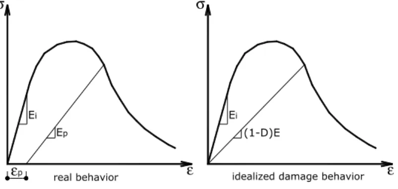
function of the strain increase. In this study, we adopted the Mazars’ damage model [24], which is grounded in the following hypotheses: damage is an isotropic variable, the residual strains are total-ly neglected, as depicted in Fig. 1 and damage occurs by tensile strains.

Figure 1 Real and idealized concrete behavior

The state of stretching at a point can be represented by the equivalent strain as:



ε

₌

( )

ε

₁

+

2

+

( )

ε

₂

+

2

+

( )

ε

₃

+

2

(7)

in which

( )

ε

_i

+ corresponds to the positive components of the main strain tensor. Thus, one has

ε

_i

( )

₊

=

⎡⎣

ε

i

+

ε

i

⎤⎦

2

, with

( )

ε

i ₊

=

ε

i in case of

ε

i

>

0

or

( )

ε

i ₊

=

0

in case of

ε

i

<

0

. The criterion to verify the material integrity at a point is given by:

f

=

ε −



_{S D}

ˆ

( )

_<

0

₍₈₎

Function

S D

ˆ

( )

_{represents the limit strain value in function of the damage. At the beginning of}

the incremental-iterative process,

S D

ˆ

( )

_{receives the strain value corresponding to the concrete}

tensile strength

ε

_{d0. In the following steps}

S D

ˆ

( )

_{is updated by the}

ε



_{value of the last step with}

damage. Due to the non symmetry of the concrete behavior in tension and compression, the damage variable is formed by the sum of two independent parts: tensile portion

D

_T and compression por-tion

D

_{C. Each of these portions indicates tensile and compression contribution to the local strain}

state and can be obtained in function of the equivalent strain and the internal parameters of the damage model as:

εp ε

σ

real behavior

Ei

Ep (1-D)E

Ei σ

ε

D

_T

=

1

−

ε

d0

(

1

−

A

T

)



ε

−

A

_T

e

⎡⎣BT(ε −ε d0)⎤⎦

D

_C

=

1

−

ε

d0

(

1

−

A

C

)



ε

−

A

_C

e

⎡⎣BC(ε −ε d0)⎤⎦

(9)

in which

ε

_d0,

_A

T,

B

T,

A

C,

B

C are the internal parameters of Mazars’ damage. Indices T and C

refer to tension and compression, respectively.

After reaching each part of the damage, the final value of the point strain state is given by

D

₌

α

_T

D

_T

₊

α

_C

D

_{C (10)}

Coefficients

α

T and

α

C can be calculated by:

α

_T

=

ε

_Ti

( )

₊

i

∑

ε

V

+

e

α

C

=

ε

_Ci

(

)

₊ i

∑

ε

V

+ (11)

in which

ε

_{Ti and}

ε

_{Ci are calculated from the main stresses considering elastic material and}

ε

_V+

represents the total state of stretching given by

ε

_V+

=

_{( )}

ε

_Ti

+

i

∑

+

₍

ε

_Ci

₎

+

i

∑

.

After damage, the stress state at the point is defined by:

σ

=

(

1

−

D

)

E

_ε

τ

=

(

1

−

D

)

G

_γ

(12)

in which

E

and

G

_{are, respectively, the longitudinal and transversal elasticity modules of the}

material and

ε

_and

_γ

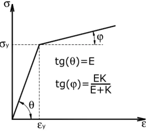
_{are, respectively, the longitudinal and transversal strains.}

3.2 Plasticity model for steel

Figure 2 Elastoplastic steel behavior

The criterion to verify the elastoplastic steel behavior is given by:

f

=

σ

s

−

(

σ

sy

+

K

α

)

<

0

(13)

in which

σ

_{s is the steel reinforcement layer stress,}

σ

sy is the steel yielding stress,

K

is the

hard-ening plastic modulus and

α

_{is an equivalent plastic strain measurement.}

The stress over each reinforcement layer can be written as:

f

≤

0

→

σ

₌

_E

ε

f

>

0

→

σ

₌

_E

t

ε

(14)

in which

E

t is the tangent elasticity modulus given by

E

t

=

EK

(

E

+

K

)

. It is interesting to note that the expression of the tangent elasticity modulus is valid only for monotonically crescent load-ing models.

4 GEOMETRIC NONLINEARITY

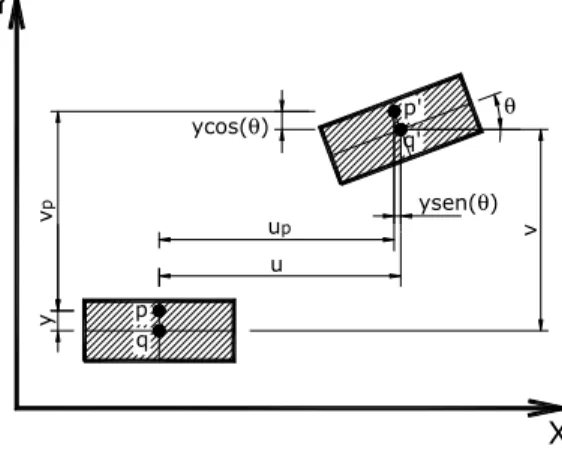
Fig. 3 illustrates the initial and final configurations of a point P in a solid after the loading action. The horizontal and vertical displacements are defined by:

θ

ϕ

tg(θ)=E

tg(ϕ)= E+K

EK

ε

σ

σ

y

Figure 3 Initial and final configuration of a point

(

)

( )

( )

(

)

( )

( )

θ

θ

cos

,

sin

,

y

y

x

v

y

x

v

y

x

u

y

x

u

p p

+

−

=

−

=

(15)

Considering a second-order approximation for small displacements, where

sinθ

₌

v

'

( )

x

_and

cos

θ

₌

1

−

v

'

2

x

( )

2

_{, one can write Eq. (15) as:}

u

_p

(

x,

y

)

=

u x

( )

−

yv'

( )

x

v

p

(

x,

y

)

=

v x

( )

−

y

v'

( )

x

2

2

(16)

in which

u

_and

v

_{correspond, respectively, to the horizontal and vertical displacement fields of any}

point of the bar.

Considering the geometric nonlinearity second-order terms given by Green strain measurement, the longitudinal and transversal strain fields,

ε

_{xx and}

_γ

xy, respectively, are written by:

ε

xx

=

∂

u

_p

∂

x

+

1

2

∂

u

_p

∂

x

⎛

⎝⎜

⎞

⎠⎟

2

+

∂

v

p

∂

x

⎛

⎝⎜

⎞

⎠⎟

2

⎡

⎣

⎢

⎢

⎤

⎦

⎥

⎥

γ

xy

=

∂

u

_p

∂

y

+

∂

v

_p

∂

x

+

∂

u

_p

∂

x

∂

u

_p

∂

y

+

∂

v

_p

∂

x

∂

v

_p

∂

y

⎛

⎝⎜

⎞

⎠⎟

(17)

Eq. (16) and (17) provide the final expression for the strains field, which is written in function of the displacements for the frame finite element:

Y X y v p up u

ysen(θ) ycos(θ)

ε

_xx

=

u

'

₊

1

2

u

'

( )

2

+

1

2

v

'

( )

2

−

yv

'' 1

(

₊

_u

'

)

γ

_xy

=

v

'

₋

_ϕ

₋

_u

'

_v

'

₋

v

'

3

2

(18)

in which

ϕ

is the additional rotation term of Timoshenko’s kinematics.

Green’s strain tensor is naturally conjugated by the second Piola-Kirchhoff stress tensor. Howev-er, in the field of small displacements and strains, the second Piola-Kirchhoff stress tensor can be replaced by the conventional stress tensor (Paula [29]):

S

=

D

₀

ε

xx

γ

_xy

⎧

⎨

⎪

⎩⎪

⎫

⎬

⎪

⎭⎪

(19)

in which

S

_{is the conventional stress tensor with longitudinal and transversal component and}

_D

0

is the material’s elastic properties tensor written as

D

0

=

E

0

0

G

⎡

⎣

⎢

⎤

⎦

⎥

.

The updated lagrangian formulation describes the structure situation based on the last balanced configuration. Thus, all the information necessary for the next load step is taken from the last con-verged step. In practical terms, this idea means two updates: positions in each node of the structure and stresses in each integration point along the finite element. The stress tensor is updated by relat-ing Cauchy’s tensor with the second Piola-Kirchhoff stress tensor. However, for small displacements and strains, Cauchy’s tensor in the current configuration coincides with the second Piola-Kirchhoff tensor of the last configuration. Thus, the update occurs simply by adding the extra stress of the current step to the last step values, as follows:

x

=

x

_a

+

Δ

x

y

=

y

_a

+

Δ

y

(20)

σ

xx

=

σ

xx_a

+

Δσ

xx

τ

xy

=

τ

xy_a

+

Δτ

xy

(21)

in which

x

_{a and}

_y

a are the nodes positions in the

x

and

y

directions of the last step,

Δ

x

and

Δ

y

are the displacements of the current step,

σ

_xx a and

τ

xya are the axial and tangential stresses of

the last step and

Δσ

_{xx and}

Δτ

5 SHEAR STRENGTH MODEL

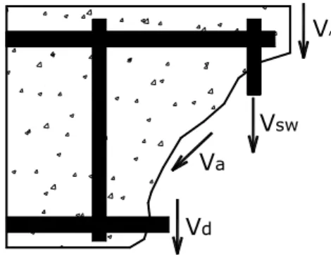
Fig. 4 shows a portion of a cracked reinforced concrete member with the shear force from each stress transfer mechanism.

Figure 4 Cracked reinforced concrete member and shear force portions

The concrete contribution,

V

_{c, is given by the}

V

_{i and}

V

_{aportions, which are related to the}

in-tact concrete and the aggregate interlock, respectively. The contributions of the longitudinal and transversal reinforcements are given by the dowel action

V

_{dand shear reinforcement}

V

_sw,

respective-ly.

5.1 Intact concrete and aggregate interlock contributions

The contributions of the concrete are given according to the criterion:

D

₌

0

→

V

_c

₌

V

_i

0

_<

D

_<

1

→

V

_c

₌

V

_a (22)

One of the mostly used forms to take into account the aggregate interlock existence is reducing the transversal elasticity modulus by a factor that depends essentially on the diagonal opening cracks (Walraven [33], Millard and Johnson [25], He and Kwan [16], Martín-Perez and Pantazopou-lou [23]). This opening crack measurement can be approximated by the main tensile strain

ε

1. Therefore, the new value of

G

_{is given by}

_µ

G

_{, where}

_µ

_{is a number between 0 and 1 that}

de-pends on

ε

1. This paper proposes to consider this reduction in function of the material damage state. It is assumed that the calibration of the damage model internal parameters in function of the tensile and compression experimental results in the concrete specimens automatically considers this effect of the aggregate interlock. As the damage variable is a function of the main strain state at a point, strain

ε

1 also influences directly the reduction in the concrete transversal stiffness. Thus, the intact concrete and the aggregate interlock strength portions are assessed by the integration of the shear stresses along the reinforced concrete finite elements cross-section as follows:

Vd

Va

V_i

V

_i

=

G

γ

_xy

dy

−h2

h2

∫

V

a

=

(

1

−

D

)

G

γ

xy

dy

−h2 h2

∫

(23)

in which

h

_{is the cross-section height.}

5.2 Dowel action contribution

The dowel action is a shear strength complementary mechanism attributed to the concrete. Howev-er, it occurs when cracks cut across the longitudinal reinforcement bars, providing an increase in the shear strength. The faces of the crack transfer shear stresses to reinforcement bars, which start a local bending and shear at the bars. The dowel action can significantly increase the shear strength, as well as the post-peak ductility of some structural elements, such as beams with few or no shear reinforcement. In this model, the reinforcement bars work as beams over the elastic foundation of the concrete. Therefore, the dowel action behavior may be affected by several factors, such as the bars position along the cross-section, concrete cover and longitudinal and transversal reinforcement ratio. Fig. 5 shows the development of the dowel forces in a reinforced concrete cracked member. The bending moment caused by the dowel action can be given by:

M

_d

₌

V

_d

L

₍₂₄₎

in which

V

_{d is the dowel shear force and}

_L

_{is the finite element length.}

Figure 5 Dowel action mechanism along the cracked reinforced concrete member

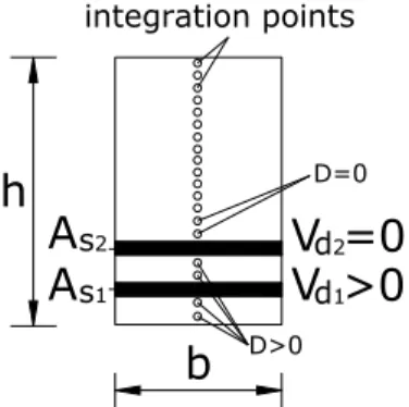
The criterion for the beginning of the dowel action contribution is given by the same damage criterion. Fig. 6 presents the proposed criterion to initiate the dowel action contribution. The exist-ence of damage is verified in the integration points immediately before and after the reinforcement layer. If the two points are damaged, that reinforcement layer will contribute to the dowel action.

Vd

Md Vd

Md

L

Δs

b h element i

Figure 6 Criterion for dowel action existence along the cross-section

He and Kwan [16] proposed an interesting formulation to estimate both the dowel force and the dowel displacement:

V

_d

₌

E

_s

I

_s

λ

3

Δ

_s

≤

V

_{du (25)}

The parameters involved in the

V

_{d calculations are:}

I

_s

₌

πϕ

s

4

64

,

λ

=

k

_c

_ϕ

_s

4

E

s

I

s

4

,

k

_c

=

127

_{c f}

c

ϕ

_s2

3 (26)

in which

E

_{s is the steel elasticity modulus,}

I

_{s is the moment of inertia of a circular cross-section}

bar,

ϕ

s is the bar diameter,

λ

is a parameter that compares the surrounded concrete stiffness with the bars stiffness,

_Δ

s is the dowel displacement,

k

c represents the stiffness coefficient of the

sur-rounding concrete,

f

_c is the concrete compression strength and

c

_{is an experimental parameter}

that reflects the spacing between the bars. Values between 0.6 and 1.0 may be assumed. In this paper 0.8 was adopted for parameter

c

_.

The dowel strength is limited by the ultimate shear capacity of the bar, which is given by:

V

du

=

1.27

ϕ

s

2

f

c

σ

sy (27)

Diameter

ϕ

s of the bars is replaced by an equivalent diameter

ϕ

s,eq calculated in function of

the reinforcement area of each layer, as:

ϕ

_s,eq

=

4

A

_s

π

(28)

b

h

A

s1

A

s2

integration points

D>0 D=0

V

_d

₌

2

π

A

s

π

E

s

I

s

λ

3

Δ

_s

≤

V

_du (29)

The dowel displacement of the cross-section of a finite element can be approximated by the arithmetic mean of the values assessed for each integration point (He and Kwan [16]), as:

Δ

s

=

π

λ

ε

1

cos

( )

α

sin

( )

α

+

γ

xy

cos

2

α

( )

⎡⎣

⎤⎦

{

}

_i

i=1

n_ht

∑

n

ht

(30)

in which

α

_{is the main tensile direction defined over the horizontal plane and}

n

_{ht is the number of} integration points along the cross-section of a finite element.

5.3 Shear reinforcement contribution

In traditional modelings with one-dimensional finite elements, the contribution of the transversal reinforcement is not considered. Therefore, it becomes necessary to introduce an approximated model to take into account its influence, especially when shear stresses cannot be neglected. In beams with high span-to-depth ratio, the bi-dimensional stress state causes an increase in the dam-age, which is assessed considering the shear and normal stresses. In these cases, the concrete quickly loses its stiffness and the presence of shear reinforcement becomes necessary to guarantee the load-ing capacity of the cross-sections. Accordload-ing to Belarbi and Hsu [4], shear reinforcement presents significant strains only after the beginning of the concrete diagonal cracking. Prior to such cracking, the stresses are resisted by both the intact concrete over the non-damaged region and the aggregate interlock mechanism over the regions of low levels of damage. For the concrete, the diagonal cracks opening is directly associated with the main tensile strain

ε

1. In the same way, the damage model

criterion is based on the presence of tension in the main strain tensor, which allows admitting that the stirrups will be loaded after the beginning of the damaging of the concrete. Thus, the criterion to initiate the shear reinforcement contribution along the loading process is given by the same dam-age criterion, as expressed in equation 8. The main idea of the model consists in transferring part of the shear force dissipated by the damaging effect to the stirrups, as depicted in Fig. 7. While the equivalent strain does not reach the limit imposed by the damage criterion, the shear force in the stirrups is zero. After reaching this limit, the total strain can be separated into two parts:

ε

₌

ε

_e

₊

ε

_{d (31)}

in which

e

_{represents the elastic strain portion and}

d

_{is the dissipated portion.}

From Eq. (12) one can write the dissipated strain portion as

ε

_d

₌

D

ε

_{. In the same way, the}

Figure 7 Scheme for stress transfer from concrete to stirrups

The Ritter-Mörsch’s truss analogy was used to calculate the stirrups transferred force portion. Sanches Jr and Venturini [30] considered the stress state of the middle point to define the stirrups strain. However, in nonlinear behavior the stirrup stresses increase from the compressed flange to-ward the tensioned flange, but decrease in the regions close to the longitudinal tensile reinforce-ment. Points localized between the cross-section central line and the closest reinforcement layer must be verified because their strains may be larger than those obtained in the cross-section middle point. To describe the equilibrium, the cross-section point with the largest strain was adopted and assessed by the maximum value of the rotated main strain damaged portion toward the reinforce-ment direction. Mathematically, one has:

ε

_sw

=

max

⎡⎣

ε

₁

D

sin

_{( )}

α

⎤⎦

₍₃₂₎

in which

ε

_{sw is the stirrups strain,}

α

_{is the main tensile direction, as depicted in Fig. 8, and max}

represents the maximum operator.

The resultant shear force in each stirrup can be assessed by

σ

_sw

A

_{sw, where}

A

_{sw corresponds to a}

single stirrup cross-section area and

σ

_{sw is the stirrup stress. This stress value is obtained by the}

elastoplastic model over strain

ε

_{sw. According to the Ritter-Mörsch’s truss analogy, the shear force}

resisted by the stirrups can be calculated for a range of width equal to the effective depth of section

d

_{. Therefore, the shear reinforcement contribution can be written as:}

V

_sw

₌

_σ

_sw

_ρ

_sw

bd

₍₃₃₎

in which

ρ

sw is the transversal reinforcement ratio defined by

A

sw

( )

sb

,

s

is the spacing between

the stirrups and

b

_{is the cross-section width.}

Unload/ Reload Load

σ_e σ

d σ

ε_e d

ε Elasti

c pre vis

ion

E

ε

E

6 SOLUTION OF THE NONLINEAR PROBLEM

The Newton-Raphson’s technique with tangent matrix was used to solve the nonlinear problem. The loading process is transformed into an incremental-iterative process, in which the stiffness ma-trix is constructed by the contribution of each integration point. Thus, the integrals expressed by Eq. (6) are converted into a discrete sum of all the material’s contributions.

The stiffness matrix of each finite element

[ ]

K

is composed of three parts: concrete bending

K

[ ]

_c,flex, concrete shear

[ ]

K

c,cis and longitudinal reinforcement

[ ]

K

s:

K

[ ]

=

[ ]

K

_c,flex

+

[ ]

K

c,cis

+

[ ]

K

s (34)

K

[ ]

_c,flex

=

B

xx,ij T

1

−

D

_ij

(

)

E

_c

B

_xx,ij

+

B

xx,ij

T

_η

ij

E

c

B

xx,ij

+

G

xx,ij

S

xx,ij

⎡

⎣

⎤

⎦

j=1

nh

∑

bh

₂

w

_y,j

⎧

⎨

⎪

⎩⎪

⎫

⎬

⎪

⎭⎪

L

2

w

x,i i=1

nl

∑

K

[ ]

c,cis

=

B

xy,ij T

1

−

D

ij

(

)

G

c

B

xy,ij

+

B

xy,ij

T

_η

ij

G

c

B

xy,ij

+

G

xy,ij

S

xy,ij

⎡

⎣

⎤

⎦

j=1

nh

∑

bh

2

w

y,j

⎧

⎨

⎪

⎩⎪

⎫

⎬

⎪

⎭⎪

i=1

nl

∑

L

2

w

x,i

K

[ ]

s

=

B

xx,ij T

E

_s

B

_xx,ij

+

G

xx,ij

σ

s,ij

⎡⎣

⎤⎦

j=1

ca

∑

A

_s,j

⎧

⎨

⎪

⎩⎪

⎫

⎬

⎪

⎭⎪

i=1

nl

∑

L

2

w

x,i

(35)

The internal forces in each finite element, i.e., normal forces

N

, shear forces

V

_{and bending}

moments

M

are obtained by:

N

₌

N

c

+

N

s (36)

V

₌

V

_l

₊

V

_a

₊

V

_d

₊

V

_{sw (37)}

M

₌

M

_c

₊

M

_s

₊

M

_{d (38)}

with:

N

_c

=

B

_xx,ij

T

1

−

D

_ij

(

)

E

_c

ε

_xx,ij

⎡

⎣

⎤

⎦

bh

₂

w

y,j j=1 nh

∑

⎧

⎨

⎪

⎩⎪

⎫

⎬

⎪

⎭⎪

L

2

w

x,i i=1

nl

∑

;

N

_s

₌

B

_xx

,ik

T

_σ

s,ik

A

s,i k₌1

ca

∑

⎧

⎨

⎩

⎫

⎬

⎭

L

2

w

_x ,i i₌1

nl

∑

;

V

l

+

V

a

=

B

xy,ij T

1

−

D

ij

(

)

G

c

γ

xy,ij

⎡⎣

⎤⎦

bh

₂

w

y,j

j=1

nh

∑

⎧

⎨

⎪

⎩⎪

⎫

⎬

⎪

⎭⎪

L

2

w

x,i i=1

nl

∑

;

V

_d

₌

2

π

A

st

π

E

s

I

s

λ

3

Δ

_s;

V

_sw

₌

_σ

_sw

_ρ

_sw

bd

_;

M

_c

=

B

_xx,ij

T

1

−

D

_ij

(

)

E

_c

ε

_xx,ij

y

j

⎡

⎣

⎤

⎦

bh

₂

w

y,j j=1 nh

∑

⎧

⎨

⎪

⎩⎪

⎫

⎬

⎪

⎭⎪

L

2

w

x,i i=1

nl

∑

;

M

s

=

B

xx,ik

T

_σ

s,ik

A

s,i k₌1

ca

∑

y

s,k

⎧

⎨

⎩

⎫

⎬

⎭

L

2

w

x,i i₌1

nl

∑

;

in which

nl

_and

nh

_{are, respectively, the number of integration points along the length and height}

of each finite element,

ca

_{is the number of longitudinal reinforcement layers in each finite element,}

E

c and

G

c are, respectively, the longitudinal and transversal elasticity modules of the concrete,

b

,

h

_and

_L

_{are, respectively, the width, height and length of each finite element,}

_y

_and

_y

s are,

re-spectively, the distances of each integration point and each reinforcement layer until the middle point of the cross-section,

A

_{s is the area of each longitudinal reinforcement layer,}

A

_{st is the sum of} all the areas of the longitudinal reinforcement layers which contribute to the dowel action and

w

x

and

w

y are, respectively, the weight-factors of each integration point on the length and height of

the finite elements,

B

xx and

B

xy are the incidence matrices containing the derivatives of the finite elements shape functions,

G

_{xx and}

_G

xy are the incidence matrices of the geometric nonlinearity.

B

xx

=

A

T

+

(

A

T

u

)

A

T

+

(

B

T

u

)

B

T

−

yC

T

−

y C

(

T

u

)

A

T

−

y A

(

T

u

)

C

T

B

xy

=

D

T

−

(

B

T

u

)

A

T

−

(

A

T

u

)

B

T

−

3

2

B

T

u

(

)

B

T

(

B

T

u

)

G

_xy

=

AA

T

+

BB

T

−

yAC

T

−

yCA

T

G

_xy

=

−

BA

T

−

AB

T

−

3

(

_B

T

_u

)

_BB

T

(39)

The strain fields are related to the nodal parameters of the finite elements through the

A

T,

B

T,

C

T_,

_D

T_{vectors, as:}

A

T

=

N

1

'

0

0

_N

₄'

0

0

⎡

⎣

⎤

⎦

B

T

=

⎡

0

_N

₂'

_N

₃'

0

_N

₅'

_N

₆'

⎣

⎤

⎦

C

T

=

⎡

0

_N

₂''

_N

₃''

0

_N

₅''

_N

₆''

⎣

⎤

⎦

D

T

=

0

−

2

g

1

₊

2

_g

(

)

L

−

_g

1

₊

2

_g

(

)

0

2

_g

1

₊

2

_g

(

)

L

−

_g

1

₊

2

_g

(

)

⎡

⎣

⎢

⎢

⎤

⎦

⎥

⎥

(40)

in which

N

_i' _and

N

_i'' _{with i = 1 to 6 are first and second derivatives of the shape functions and}

_g

is the Weaver’s constant, which is

g

₌

6

_EI

0.833

_GAL

_{for the rectangular cross-sections.}

N

1

=

1

−

x

L

⎛

⎝⎜

⎞

⎠⎟

;

N

2

=

1

−

3

x

L

⎛

⎝⎜

⎞

⎠⎟

2

+

2

x

L

⎛

⎝⎜

⎞

⎠⎟

3

⎡

⎣

⎢

⎤

⎦

⎥

;

N

3

=

L

x

L

⎛

⎝⎜

⎞

⎠⎟

−

2

x

L

⎛

⎝⎜

⎞

⎠⎟

2

+

x

L

⎛

⎝⎜

⎞

⎠⎟

3

⎡

⎣

⎢

⎤

⎦

⎥

N

4

=

x

L

⎛

⎝⎜

⎞

⎠⎟

;

N

5

=

3

x

L

⎛

⎝⎜

⎞

⎠⎟

2

−

2

x

L

⎛

⎝⎜

⎞

⎠⎟

3

⎡

⎣

⎢

⎤

⎦

⎥

;

N

6

=

L

−

x

L

⎛

⎝⎜

⎞

⎠⎟

2

+

x

L

⎛

⎝⎜

⎞

⎠⎟

3

⎡

⎣

⎢

⎤

⎦

⎥

(41)

in which

x

_{corresponds to any horizontal coordinate along the finite element length.}

The

η

function considers the equivalent strain derivatives related to the strain components and is assessed by:

η

₌

_F

_{( )}

_ε



∂

ε



∂

_ε

(42)

According to Mazars’ damage model,

F

_{( )}

ε



_{is a linear combination of the tensile and} compres-sion damaging functions obtained with

F

( )

ε



₌

α

_T

F

T

( )

ε



+

α

C

F

C

( )

ε



.

F

_T

_{( )}

ε



₌

ε

d0

(

1

−

A

T

)



ε

2

+

A

_T

B

_T

e

⎡⎣BT(ε−ε d0)⎤⎦

F

_C

( )

ε



₌

ε

d0

1

−

A

_C

(

)



ε

2

+

A

_C

B

_C

e

⎡⎣BC(ε−ε d0)⎤⎦

(43)

The derivative of the equivalent strain related to the horizontal portion of the strain tensor de-pends on the directions of the fiber strains according to:

∂

ε



∂ε

_x

=

1

(tension) ou

∂

ε



A complete flowchart for the entire proposed FEM model is illustrated in Fig. 8. The boxes with a numerical index are explained in details because they describe the most important parts of the program, including all the developed particular models.

1 – Initial Data: in this section, one can check the models which will be considered in the numerical analysis, such as dowel action, shear reinforcement contribution, Euler-Bernoulli or Timoshenko’s theory and the finite element mesh description;

2 – Starting Incremental Process: in this section, the program applies the load or displacement in-crement on the particular nodes of the mesh;

3 – Starting Iterative Process: in this section, the program starts the iterative process preparing all the internal variables of the damage and plasticity models, as well as the shear strength mecha-nisms;

4 – Local Stiffness Matrix: in this section, the stiffness matrix of each finite element is calculated, considering local degradation state and local plasticization state of the integration Gauss points on the cross-section and longitudinal reinforcement layers along the finite elements, respectively. The local stiffness matrix is evaluated by Eq. 34, in which the separated parts for concrete (bending and shear) and for longitudinal reinforcements steel are given by [K]c,flex, [K]c,cis and [K]s, respectively (evaluated by Eq. 35). Each of the variables used in these equations was already described, depend-ing of the adopted shape functions and their derivatives, mechanical properties of the materials, geometry of the structure and internal variables of the damage and plasticity models (as described by Eq. 39 to 44).

5 – Internal Forces Assessment: in this section, the internal resistances forces are assessed taking into account material behaviors and shear complementary mechanisms, which are aggregate inter-lock and dowel action, as well as the contribution of shear reinforcement. The internal forces given by the normal force, shear force and bending moment in each cross-section over all the discretiza-tion points along the finite element length are assessed by Eq. (36), (37) and (38), respectively. It is necessary to identify each component of these calculations: Nc and Ns are the contributions of

un-damaged concrete and longitudinal reinforcement for normal forces; Vl and Va are the contributions

of undamaged concrete and aggregate interlock, respectively; Vd and Vsw are the contributions of

the dowel action and shear reinforcement assessed by the developed models, respectively; Mc, Ms

and Md are the contributions of concrete, longitudinal reinforcement and the bending moment from

dowel action, respectively.

 

1 - Initial Data

2 - Starting Incremental Process

Application of load/displacements increments

3 - Starting Iterative Process

4 - Local Stiffness Matrix

Global Stiffness Matrix

Boundary Conditions

SOLVE Linear System of Equations

Update Nodal Displacements

5 - Internal Forces Assessment

Residual Forces Vector Assessment

Convergence Verification

No

Yes

Update Nodal Coordinates

All the Load Steps?

Yes No

7 NUMERICAL APPLICATIONS

The common information to all the numeric examples is: force and displacement convergence toler-ance to verify the equilibrium is 10-4; 6 and 20 integration points along the length and the cross-section of the finite elements, respectively. Value of the KS parameter for the elastoplastic behavior

of the steel reinforcements is, in both examples, 10% of ES.

7.1 Example 1

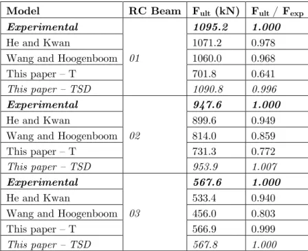
In this example three reinforced concrete beams with same geometry and loading, but different lon-gitudinal and transversal reinforcement ratios were analyzed. The beams were experimentally tested by Ashour [1] and numerically tested by He and Kwan [16]. They considered the steel bars embed-ded in a quadrilateral isoparametric finite element (plain stress state) of concrete with two extra degrees of freedom for bending to eliminate the shear locking. The ultimate loads were compared with the results of Wang and Hoogenboom [34], who simulated beams from a stringer-panel bi-dimensional mechanical model, in which the cracked concrete was considered an orthotropic materi-al. The reinforcement details, as well the mesh of 18 finite elements with different lengths are shown in Fig. 9. The mechanical parameters used for each beam are given in Table 1.

Table 1 Concrete and steel properties

RC Beam fc (MPa) Ec (MPa) νc fs (MPa) Es (MPa) Ks (MPa)

01 30.0 25921 0.24 500 205000 20500

02 33.1 27227 0.23 500 205000 20500

03 22.0 22198 0.26 500 205000 20500

The parameters of the damage model ε_d0, A_T, B_T, A_C and B_C were calibrated for each concrete compression strength and are given in Table 2. The mechanical models used in these analyses took into account the Timoshenko’s theory only with the concrete contributions, i.e., intact concrete and aggregate interlock (T) and the full Timoshenko’s theory with all the contributions (TSD).

The results of the analysis are depicted in Fig. 10, 11 and 12. It is possible to verify a considera-ble difference between the results of the T and TSD models in the two first beams, which shows the importance of the stress transfer from the cracked concrete to the shear reinforcement.

Table 2 Parameters of the damage model

fc (MPa) εd0 AT BT AC BC

30.0 0.000078 1.004 9000 1.056 1034

33.1 0.000080 1.018 8997 1.048 963.3

From the point of view of the equilibrium trajectory, the 1D FEM model considering TSD showed, for beam 01, a better behavior than that observed with the He and Kwan [12] 2D FEM model, as depicted in Fig. 10. The Mazars’ damage model tends to produce better results for rein-forced concrete members with higher reinforcement rates than for concrete members with lower reinforcement rates. Such a behavior is due to the damaging along the concrete member producing a better representation of the real cracking panorama. Moreover, the aggregate interlock defined by the damage model proved to be better considered in this case and also in the ultimate load and TSD was more accurate than the others, as seen in Table 3.

For beam 02, all the numerical modeling showed a more rigid behavior than the experimental re-sults. The withdrawal of two reinforcement layers closer to the beam’s geometric center and the largest vertical spacing between the layers demonstrated importance in the description of the equi-librium trajectory, but they did not provide a good agreement with the experimental results. How-ever, in terms of ultimate load, the TSD model reached almost the same value obtained in the ex-perimental test, as illustrated in Table 3.

Beam 03 presented almost the same result for the T and TSD models, since there was no shear reinforcement. The shear strength in this case was given by the intact concrete, aggregate interlock and dowel action portions. The dowel action influence was found to be small when compared to the shear transversal reinforcement. Therefore, the shear reinforcement together with the concrete con-tributions is responsible for the shear strength in deep reinforced concrete beams. The ultimate load value provided by the dowel action was different from the value observed in the T model (Table 3), indicating a small contribution to the final shear strength of the beam.

Table 3 Values of the ultimate load

Model RC Beam Fult (kN) Fult / Fexp

Experimental

01

1095.2 1.000

He and Kwan 1071.2 0.978

Wang and Hoogenboom 1060.0 0.968

This paper – T 701.8 0.641

This paper – TSD 1090.8 0.996 Experimental

02

947.6 1.000

He and Kwan 899.6 0.949

Wang and Hoogenboom 814.0 0.859

This paper – T 731.3 0.772

This paper – TSD 953.9 1.007 Experimental

03

567.6 1.000

He and Kwan 533.4 0.940

Wang and Hoogenboom 456.0 0.803

This paper – T 566.9 0.999

Figure 9 Geometry, loading and discretization of the analyzed beams

Stirrups:

φ8 c/ 100 Beam 01: 2φ10 4φ12 4φ12 2φ10 4φ8 F F 3000 160

495 165 680 680 165 495

160 120 625 CG 45.1 32 31 102.1 32 45.1 Stirrups:

φ8 c/ 200 Beam 02: 2φ10 102.1 117.8 117.8 4φ12 4φ12 2φ10 4φ8 F F 3000 160

495 165 680 680 165 495

160 120 625 CG 45.1 32 31 102.1 32 45.1 Stirrups: none Beam 03: 2φ10 102.1 117.8 117.8 625 625 625 F F

Dimensions in millimeters

4φ12 4φ12 2φ10 8φ8 F F L=160 Le=160 Le=165 Le=165 Le=170

Finite elements mesh

node 1 node 6 node 14 node 19

3000 160

495 165 680 680 165 495

Figure 10 Equilibrium trajectory of vertical node 14: beam 01

Figure 13 Equilibrium trajectory of vertical node 14: beam 03

7.2 Example 2

The structure studied in this example is a reinforced concrete frame tested by Vecchio and Emara [32] and numerically analyzed by Güner [15] and La Borderie et al. [20]. The considered models were Euler-Bernoulli (B) without shear contributions and full Timoshenko’s (TSD). The loads and frame geometry are depicted in Fig. 13.

Figure 13 Geometry and loads of the reinforced concrete frame

900 700kN

900

400 3100 400

40

0

18

00

40

0

16

00

40

0

700kN

F

B B B B

A A

A A

Dimensions in millimeters

300

40

0

30

0

50

50

φ10 c/ 125 Stirrups:

4φ20 4φ20 Section BB:

300

40

0

32

0

40

40

φ10 c/ 125 Stirrups:

4φ20 4φ20 Section AA:

C C

800

40

0

28

0

60

60

φ10 c/ 250 Stirrups:

Two types of support conditions were considered: case I – frame with a support beam and case II – clamped-clamped frame, as shown in Fig. 13. The response obtained by La Borderie et al. [20] was considered only for case II and repeated for case I. Concerning the types of analyses, Güner [15] used the SAP 2000 [8] software, in which the structure is considered with a mixed behavior, i.e., elastic-linear along the one-dimensional finite elements and plastic hinges at the appropriate mem-ber ends. These hinges are positioned at the end nodes of some special finite elements, such as the joint of a beam and column to simulate the existence of rigid offsets. The La Borderie et al. [20] modeling was performed with one-dimensional finite elements, but with their own damage model, in which the inelastic strains from the damage were taken into account.

Figure 14 Cases of the support conditions considered

The parameters used were concrete elasticity modulus of 23674MPa, concrete compression strength of 30MPa, concrete Poisson’s ratio of 0.2, steel yielding stress of 418MPa, steel elasticity modulus of 192500MPa and steel plastic modulus of 19250MPa. The horizontal loading on the frame top was applied in steps of 5kN. The damage parameters were, respectively, ε_d0, A_T, B_T, A_C, and BC: 0.000085; 1.145; 10330; 1.117 and 1189. The equilibrium trajectories for cases I and II are

depicted in Fig. 15 and 16.

1 6 2 7 11 12 16 15 14 13 3 4 5

8 9 10 17

18 19 20 21

22 23 24 25 26 27 28 29 30 31

32 33 34 35 36 37 38 39 40 41 42 43 Case I 1 6 2 7 11 12 16 15 14 13 3 4 5

8 9 10 17

18 19 20 21

22 23 24 25 26 27 28 29 30 Case II 0 50 100 150 200 250 300 350 400

0 1 2 3 4 5 6 7 8 9

Lateral displacement, cm

La te ra l loa d, k N

The use of clamped supports, as observed in case II, provided higher stiffness to the structure, since there was no rotation in the support nodes. The support beams adopted in case I did not show a significant difference for model B. However, for the TSD model, some changes were observed in terms of displacements after concrete cracking and especially in terms of ultimate load. The great capacity of internal forces redistribution may be the main reason for this behavior.

Figure 16 Horizontal equilibrium trajectory of node 21: case II

Tables 4 and 5 present the values of the loading and horizontal displacement for both reinforce-ment steel yielding in node 1 and frame ruin. The column Error (%) was evaluated from a compari-son between experimental and each numerical result for both yielding and ultimate loads.

Table 4 Comparison between the results: case I

Model Yielding Ultimate

F (kN) d (cm) Error (%) F (kN) d (cm) Error (%) Experimental 264.0 2.68 0.0 332.0 8.21 0.0

Güner [15] with SAP2000 238.0 1.89 -9.8 309.0 8.06 -6.9

La Borderie et al. [20] 277.0 2.53 +4.9 373.0 8.64 +12.3

B 285.0 2.88 +7.9 355.0 8.20 +6.9

TSD 265.0 2.85 +0.4 320.0 8.31 -3.6

Table 5 Comparison between the results: case II

Model Yielding Ultimate

F (kN) d (cm) Error (%) F (kN) d (cm) Error (%) Experimental 264.0 2.68 0.0 332.0 8.21 0.0

Güner [15] with SAP2000 238.0 1.89 -9.8 309.0 8.06 -6.9

La Borderie et al. [20] 277.0 2.53 +4.9 373.0 8.64 +12.3

B 285.0 2.86 +7.9 365.0 8.27 +9.9

TSD 283.0 2.80 +7.2 360.0 8.10 +8.4 0

50 100 150 200 250 300 350 400

0 1 2 3 4 5 6 7 8 9

Lateral displacement, cm

La

te

ra

l

loa

d,

k

N

As one can observe, the TSD model for case I represented better the real behavior of the frame in terms of ultimate load and reinforcement steel yielding, showing differences of only -3.6% and +0.4%, respectively, in comparison to the experimental tests. In the case II, in which the structure is considered as a clamped-clamped frame, the proposed model was capable to obtain a good agree-ment compared to the other models regarding the experiagree-mental results, especially for the ultimate load.

8 CONCLUDING REMARKS

This paper presented a mechanical model based on the one-dimensional finite element method which incorporates the shear reinforcement strength, the dowel action and the aggregate interlock from the concepts of the damage mechanics, besides the geometric nonlinearity. One of its ad-vantages consists in adapting the shear strength mechanisms for a bar finite element without 2D analysis. The results allowed concluding that the model could satisfactorily represent a structural behavior in which the influence of the shear strains must be considered, highlighting the contribu-tions of the shear reinforcement, dowel action and aggregate interlock. The aggregate interlock por-tion was assessed together with the intact concrete porpor-tion given by the damage model. Thus, by calibrating the damage parameters, the aggregate interlock was automatically taken into account, because these parameters are obtained from the experimental tests of the concrete. The coupling between the shear strength complementary mechanisms, the damage model for concrete and geo-metric nonlinearity is also another interesting aspect. It allowed simulating frame structures, which take the equilibrium in the deformed configuration with the stiffness loss from bending and shear strain states. Finally, the model has showed numerical stability and capability of assessing the ulti-mate loads, the start of concrete cracking and the reinforcement steel yielding values of the ana-lyzed structures with good accuracy.

Acknowledgements The authors would like to acknowledge FAPESP (São Paulo Research Foundation) for the financial support given to this project. A special “thanks” to professor W. S. Venturini (in memoriam).

References

[1] ASHOUR, A.F. Tests of reinforced concrete continuous beams. ACI Structural Journal, v.97, n.1, p.3-12; 1997. [2] BATHE, J.K. Finite element procedures in engineering analysis. Prentice-Hall, Englewood Cliffs; 1982.

[3] BAZANT, Z.P.; GAMBAROVA, P.G. Rough cracks in reinforced concrete. Journal of the Structural Division, ASCE, v.106, n.4, April, p.819-842; 1980.

[4] BELARBI, A.; HSU, T.T.C. Stirrup stresses in reinforced concrete beams. ACI Structural Journal, September-October, p.530-538; 1990.

[5] BELLETTI, B.; CERIONI, R.; IORI, I. Physical approach for reinforced-concrete (PARC) membrane ele-ments. Journal of Structural Engineering, ASCE, v.127, n.12, December, p.1412-1426; 2001.

[6] BHATT, P.; KADER, M.A. Prediction of shear strength of reinforced concrete beams by nonlinear finite ele-ment analysis. Computers and Structures, v. 68, p. 139-155; 1998.

[7] CLOUGH, R.W.; PENZIEN, J. Dynamics of structures. 2nd Edition; 1993.