A FAULT DETECTION AND ISOLATION SYSTEM FOR COOPERATIVE
MANIPULATORS
Renato Tin´os
∗ [email protected]Marco Henrique Terra
†∗Departamento de F´ısica e Matem´atica, FFCLRP - Universidade de S˜ao Paulo (USP), Ribeir˜ao Preto, SP, 14040-901, Brasil †Departamento de Engenharia El´etrica, EESC - Universidade de S˜ao Paulo (USP), S˜ao Carlos, SP, 13560-970, Brasil
ABSTRACT
The problem of fault detection and isolation (FDI) in coop-erative manipulators is addressed in this paper. Four FDI procedures are developed to deal with free-swinging joint faults, locked joint faults, incorrectly measured joint posi-tion, and incorrectly measured joint velocity. Free-swinging and locked joint faults are isolated via neural networks. For each arm, a Multilayer Perceptron (MLP) is used to repro-duce the dynamics of the fault-free robot. The outputs of each MLP are compared to the actual joint velocities in or-der to generate a residual vector which is then classified by an RBF network. The remaining faults are isolated based on the kinematic constraints imposed on the cooperative system. Results obtained via simulations and via an actual coopera-tive manipulator robot are presented.
Keywords:Fault Detection, Fault Isolation, Robotic Manip-ulators, Co-operation, Neural Networks.
1
INTRODUCTION
The actuation areas of Robots have been spreading from in-dustries and laboratories into hospitals, deep sea, outer space, nuclear facilities, and other hazardous, unstructured, or hard-to-reach environments. In these environments, robots are employed to avoid the exposition of human beings to dan-ger or because of the reliability of robots in executing
repet-Artigo submetido em 27/03/2007 1a. Revis ˜ao em 14/10/2008
Aceito sob recomendac¸ ˜ao do Editor Associado Prof. Jos ´e Reinaldo Silva
itive tasks. However, faults in robots, which are not unusual due to their inherent complexity, can put at risk the robot, its mission, and the working environment.
There are several sources of faults in robots, such as elec-trical, mechanical, hydraulic, and of software (Visinsky et al., 1994). There are good reasons to research and to de-velop fault detection and isolation (FDI) systems for robots, in particular to improve their safety to work among humans.
Robotic systems with kinematic or actuation redundancy are interesting in applications where the fault problem should be addressed because the number of degrees of freedom (dof) in these systems is greater than the dof required to manipulate the load. Actuation redundancy can be found in only closed-link mechanisms as cooperative systems formed by two or more arms (Nakamura, 1991). As in the humans, where the use of two arms presents an advantage over the use of only one arm in several cases, two or more robots can execute tasks that are difficult or even impossible for only one robot (Vukobratovic and Tuneski, 1998). Examples of such tasks include the manipulation of heavy, large or flexible loads, assembly of structures, and manipulation of objects that can slide from only one robot end-effector.
caus-ing damage to the load and instability in the cooperative sys-tem (Tin´os et al., 2006).
This work develops an FDI scheme for cooperative robots rigidly connected to an undeformable load based on pro-cedures to isolate four kind of faults: free-swinging joint faults (FSJFs), locked joint faults (LJFs), incorrectly mea-sured joint position faults (JPFs), and incorrectly meamea-sured joint velocity faults (JVFs). The faults are detected and iso-lated as follows:
a) JPFs and JVFs are detected and isolated based on kine-matics constraints imposed by the closed kinematic chain. If the number of armsmin the cooperative system is greater than two (m > 2) and supposing that only one fault occurs each time, the manipulator with the wrong measurement can be direcly detected by checking the estimates of the load po-sition (or velocity for JVFs) obtained for each arm. Then, the estimate of each joint position (or velocity for JVFs) of the faulty arm is computed and compared to its measurement in order to isolate the fault. Ifm= 2, the arm with the wrong measurement cannot be identified just by checking the esti-mate of position (or velocity) of the load obtained for each arm. In this case, the estimate of the joint position (or veloc-ity) should be done for all arms.
b) FSJFs and LJFs are detected by artificial neural networks (ANNs). The dynamics of the arms are mapped by Multi-layer Perceptrons (MLPs), which produces outputs that are compared to actual velocity measurements in order to gener-ate the residual vector. Then, a Radial Basis Function Net-work (RBFN) is utilized to classify the residual vector.
This paper is organized as follows: Section 2 describes the kinematics and dynamics of cooperative manipulators; Sec-tion 3 describes the FDI system; SecSec-tion 4 presents the re-sults of the FDI system in simulations and in an actual co-operative robot with two arms; finally, the conclusions are presented in Section 5.
2
COOPERATIVE MANIPULATORS
The equation of motion for thei-th arm in a fault-free multi-robot system with mrobots rigidly connected to an unde-formable load is given by
Mi(qi)¨qi+gi(qi) +Ci(qi,q˙i)q˙i =τi−Ji(qi)
T hi (1)
whereqiis the vector of joint angles of armi,i= 1, . . . , m, τi is the vector of applied torques at the joints of arm i,
Mi(qi)is its inertia matrix,Ci(qi,q˙i)is its matrix of
cen-trifugal and Coriolis terms,gi(qi)is its vector of
gravita-tional terms, Ji(qi) is the geometric Jacobian (from joint
velocity to end-effector velocity) of armi,hi = [fiTη
T
i]
T is the force vector at the end-effector of armi,fiis the vector of
spatial forces at the end-effector of armi, andηiis the
vec-tor of vec-torques at the end-effecvec-tor of armi; the friction terms were not shown for simplicity. The combined dynamics of all arms can be written in only one equation as
M(q)¨q+g(q) +C(q,q˙)q˙ =τ−J(q)T
h (2)
whereq= [qT
1 q
T
2 . . . q
T
m]
T
,τ = [τT
1 τ
T
2 . . . τ
T
m]
T ,h=
[hT1 hT2 . . . hTm]T
,M(q)is formed by the individual inertia matrices of the arms,C(q,q˙) is formed by the individual centrifugal and Coriolis matrices of the arms,g(q)is formed by the individual gravitational terms of the arms, andJ(q)is formed by the termsJi(qi)fori= 1, . . . , m.
The equation of motion for the manipulated object (load) is given by
Mov˙o+bo(xo,vo) =Jo(xo) T
h (3)
wherexo = [p T o φ
T o]
T
is the k-dimensional vector of po-sition and orientation at the origin of the frame attached to the center of mass of the load (frame CM),pois the vector of load position,φois the minimal representation of orienta-tion of the load,vo = [p˙
T o ω
T o]
T
is the vector of linear and angular velocities of the load,bo is the vector of centrifu-gal, Coriolis, and gravitational terms,Mois the load inertia matrix, andJo(xo) =
Jo1(xo) T
. . . Jom(xo)
T T
, whereJoi(xo)converts velocities of the load into velocities of the end-effector of armi. In the three-dimensional space, po= [xo yo zo]
T
, and either Euler angles or RPY (Roll-Pitch-Yaw) angles can be chosen as the minimal representa-tion of the load orientarepresenta-tion, i.e.,φo= [ϕoυoψo]
T
. The ve-locitiesvocan be calculated byvo =T(xo)x˙o(Sciavicco and Siciliano, 1996), whereT(xo)is a transformation ma-trix used to relate the angular velocities to the derivative of the minimal representation of the orientation (euler angles or RPY angles) in the 3-dimensional space (T(xo) = Ifor planar manipulators, whereIis the identity matrix).
As it is possible to compute the positions and orientations of the load using the positions of the joints of any arm of the cooperative system, the following kinematic constraint appears
xo=ϕ1(q1) =ϕ2(q2) =. . .=ϕm(qm) (4)
whereϕi(qi)is the vector of the position and orientation of
the load computed via the joint positions of armi, i.e., the direct kinematics of armi. The velocities of the load are constrained by
vo=D1(q1)q˙1 =D2(q2)q˙2 =. . .=Dm(qm)q˙m (5)
whereDi(qi) = Joi(xo)− 1
Ji(q) is the Jacobian relating
The squeeze forces are given by (Wen and Kreutz-Delgado, 1992)
hos=Ps(xo)h (6)
where the matrixPs(xo) transforms forces and torques in the end-effectors into squeeze forces in the load.
Several solutions have been proposed to deal with the control problem in fault-free cooperative manipulators rigidly con-nected to an undeformable load as the master/slave strategy (Luh and Zheng, 1987), the optimal division of the load con-trol (Carignan and Akin, 1988), (Nahon and Angeles, 1992), the definition of new task objectives or variables (Koivo and Unseren, 1991), (Caccavale, 1997), and the hybrid control of motion and squeeze in the object (Uchiyama, 1998), (Wen and Kreutz-Delgado, 1992), (Bonitz and Hsia, 1996).
3
FDI SYSTEM
The FDI system is proposed based on the following faults: FSJF, where an actuation loss occurs in one arm joint (English and Maciejewski, 1998); LJF, where one arm joint is locked (Goel et al., 2004); JPF, where the measurement of the joint position is not correct (Notash, 2000), and JVF, where the measurement of the joint velocity is not correct. JPFs and JVFs generally occur due to sensor faults. By sim-plicity, the occurrence of only one fault at a time is consid-ered. A three step FDI system is applied here in each sample time. First, JPFs are detected by analyzing the position con-straints (Eq. 4). Then, JVFs are detected by analyzing the velocity constraints (Eq. 5). The last step is the detection of FSJFs and LJFs via ANNs. This sequence is important be-cause undetected JPFs can be-cause the false detection of other faults as joint position measurements are used in Eq. (5) and as inputs of the ANNs. The same occurs for undetected JVFs in FSJFs and LJFs as joint velocity measurements are used as inputs of the ANNs.
3.1
Incorrectly Measured Joint Position
Faults (JPFs)
In (Notash, 2000), the direct kinematics is used to detect joint position sensor faults in parallel manipulators. The direct kinematics problem (knowing the joint positions, identify the position and orientation of the load) is not trivial in paral-lel manipulators because they have one or more unsensed joints. The direct kinematics problem is, however, easier in cooperative manipulators because all joints are assumed to be equipped with sensors. The problem of fault tolerance in parallel manipulators is still addressed in (Hassan and No-tash, 2004) and (Hassan and NoNo-tash, 2005).
In this work, the direct kinematics and the kinematic con-straints imposed by the closed chain are used to detect JPFs
in cooperative manipulators. Two cases are considered:
whenm = 2orm > 2, i.e., there are two or more than
two manipulators in the cooperative system.
3.1.1 JPFs whenm >2
Asxocan be calculated using the joint positions of any arm (Eq. 4), it is possible to identify the armf with the wrong joint position measurements ifm >2. A wrong estimate of the load positionxois produced by the arm with the wrong measurements, which differs from the estimate of the other
m−1arms. A JPF is detected in armfif
kˆxof(θf)−ˆxoi(θi)k> γp1
for alli= 1, . . . , mandi6=f (7)
whereˆxoi(θi)is the estimate ofxousing the measurements
θi of the joint positionsqi in armi,θf is the vector of the
measured positions of the joints in armf,k.krepresents the Euclidean norm, and the thresholdγp1is adjusted by the
de-signer to avoid that false alarms appear due to the presence of noise in the joint measurements. The next step is to estimate the position of each jointj= 1, . . . , nf of armf
ˆ
qf j =ψpj(θf,ˆxo) (8)
whereψpj is the kinematic function used to estimate the po-sition of jointj, and
ˆ xo=
1 m−1
m
X
i=1,i6=f
ˆ xoi(θi).
Calculating again the estimate of vector xo for arm f for each new estimateqˆf j, the JPF in jointjof armf is detected when
kˆxo−ˆxof(θf,ˆqfj)k< γp2 (9)
wherexˆof(θf,ˆqfj)is the vector of positions and orientations of the load estimated for armfsubstituting the measured po-sition of jointj by its estimateqˆf j and using the measured positions of the other joints. The thresholdγp2is adjusted by
the designer to avoid that faults are hidden due to the pres-ence of noise in the joint measurements.
The procedure to detect and to isolate JPFs whenm >2can be summarized as follows: compare the estimate ofxofor all arms (Eq. 7); if all values are close, a JPF is not announced, otherwise, calculate for all joints of the faulty arm the esti-mate of the joint positions (Eq. 8), and test Eq. (9) for all joints; if the test is satisfied for jointj, announce a JPF in this joint.
3.1.2 JPFs whenm= 2
by comparing the two estimates ofxo. In this way, a JPF is detect whenm= 2if
kˆxo1(θ1)−xˆo2(θ2)k> γp1. (10)
As it is not possible to identify the arm with the fault, the joint positions estimate (Eq. 8) should be done for all joints in the two arms using, instead of the the value ofˆxo, the estimate obtained using the joint positions of the other arm. For arm
1, the position of the jointj= 1, . . . , n1 is estimated by
ˆq1j =ψpj(θ1,ˆxo2(θ2)) (11)
and, for arm2, the position of the joint j = 1, . . . , n2 is
estimated by
ˆq2j =ψpj(θ2,ˆxo1(θ1)). (12)
Calculating again the estimate of vectorxofor each new es-timate of joint position (eqs. 11 and 12), the JPF in jointjof arm1is detected when
kxˆo1(θ1,ˆq1j)−ˆxo2(θ2)k< γp2 (13)
whereˆxo1(θ1,ˆq1j)is the vector of positions and
orienta-tions of the load estimated for arm1 substituting the mea-sured position of joint j by its estimateqˆ1j and using the measured positions of the other joints, and the JPF in jointj
of arm2is detected when
kxˆo1(θ1)−ˆxo2(θ2,ˆq2j)k< γp2 (14)
whereˆxo2(θ2,ˆq2j)is the vector of positions and orienta-tions of the load estimated for arm2 substituting the mea-sured position of joint j by its estimateqˆ2j and using the measured positions of the other joints
3.2
Incorrectly Measured Joint Velocity
Faults (JVFs)
As it is possible to calculate the velocity of the load by using the joint velocities of any arm (Eq. 5), JVFs can be detected in a similar way of JPFs.
3.2.1 JVFs whenm >2
By using Eq. (5), it is possible to identify the arm f with the wrong joint velocity measurements ifm > 2. A JVF is detected in armfif
kvˆof(θ˙f,θf)−ˆvoi(θ˙i,θi)k> γv1
for alli= 1, . . . , mandi6=f (15)
wherevˆoi(θ˙i,θi)is the estimate ofvousing the measured velocitiesθ˙iand the measured positionθiof the joints in arm
i,θ˙f is the vector of the measured velocities of the joints in
armf, and the thresholdγv1 is adjusted by the designer to
avoid that false alarms appear due to the presence of noise in the joint measurements. The next step is to estimate the velocity of each jointj= 1, . . . , nf of armf
ˆ˙qf j=ψvj(θ˙f,θf,ˆvo) (16)
whereψvj is the kinematic function used to estimate the ve-locity of jointj, and
ˆ vo=
1 m−1
m
X
i=1,i6=f
Di(θi)θ˙i.
Calculating again the estimate of vectorvo for arm f for each new estimateˆ˙qf j, the JVF in jointjof armfis detected when
kˆvo−vˆof(θ˙f,θf,ˆ˙qfj)k< γv2 (17)
wherevˆof(θ˙f,θf,ˆ˙qfj)is the vector of velocities of the load
estimated for arm f substituting the measured velocity of jointj by its estimateˆ˙˙qf j and using the measured veloci-ties of the other joints. The thresholdγv2 is adjusted by the
designer to avoid that faults are hidden due to the presence of noise in the joint measurements.
The procedure to detect and to isolate JVFs whenm > 2
can be summarized as follows: compare the estimate ofvo for all arms (Eq. 15); if all values are close, a JVF is not announced, otherwise, calculate for all joints of the faulty arm the estimate of the joint velocities (Eq. 16), and test Eq. (17) for all joints; if the test is satisfied for jointj, announce a JVF in this joint.
3.2.2 JVFs whenm= 2
Ifm= 2, the faulty arm cannot be identified just by checking the estimates ofx˙o. However, it is possible to detect a JVF by comparing the two estimates ofx˙o. In this way, a JVF is detect whenm= 2if
kvˆo1(θ˙1,θ1)−vˆo2(θ˙2,θ2)k> γv1. (18)
As it is not possible to identify the arm with the fault, the joint velocities estimate (Eq. 16) should be done for all joints in the two arms using, instead of the the value ofˆ˙xo, the estimate obtained using the joint velocities of the other arm. For arm1, the velocity of the jointj= 1, . . . , n1is estimated
by
ˆ˙
q1j =ψvj(θ˙1,θ1,ˆvo2(θ˙2,θ2)) (19)
and, for arm2, the velocity of the jointj = 1, . . . , n2 is
estimated by
ˆ˙
Calculating again the estimate of vectorx˙ofor each new es-timate of joint velocity (eqs. 19 and 20), the JVF in jointjof arm1is detected when
kvˆo1(θ˙1,θ1,ˆ˙q1j)−ˆvo2(θ˙2,θ2)k> γv2. (21)
whereˆvo1(θ˙1,θ1,ˆ˙q1j)is the vector of velocities of the load
estimated for arm 1 substituting the measured velocity of jointj by its estimateˆ˙q1j and using the measured velocities of the other joints, and the JVF in jointjof arm2is detected when
kvˆo1(θ˙1,θ1)−vˆo2(θ˙2,θ2,ˆ˙q2j)k> γv2. (22)
whereˆvo2(θ˙2,θ2,ˆ˙q2j)is the vector of velocities of the load
estimated for arm 2 substituting the measured velocity of jointj by its estimateˆ˙q2j and using the measured velocities of the other joints.
3.3
Free-Swinging Joint Faults (FSJFs)
and Locked Joint Faults (LJFs)
As FSJFs and LJFs introduce dynamic effects in the coop-erative system, the residual generation and analysis concept can be used to detect and isolate these faults (Isermann and Ball´e, 1997). In the residual generation, the mathematical model is generally used to reproduce the dynamic behavior of the fault-free system. The deviation of the output predicted by the model from actual output measurements forms the so-called residuals which, when properly analyzed, provides valuable information about the failures. Modeling errors, however, may obscure the effects of some faults and can be a source of false alarms (Gertler, 1997). To solve this problem, robust FDI schemes have been proposed (Mangoubi, 1998), (Chen and Patton, 1999).
Alternatively, one may resort to artificial intelligence tech-niques like knowledge-based systems, fuzzy logic, and ANNs. ANNs have been employed for FDI mainly in static systems, and less intensively in dynamic systems (Korbicz, 1997). In most applications, ANNs are used as classifiers based on measurements of the process output. In dynamic systems, however, the outputs are affected by the inputs and, therefore, this procedure generally is not valid. An alter-native is to employ the residual generation concept, where one ANN is used as a classifier based on the residuals pro-duced by the system mathematical model or by another ANN (K¨oppen-Selinger and Frank, 1996).
FDI for individual manipulators has been typically pursued employing the robot mathematical model for residual gen-eration (Visinsky et al., 1994). For residual analysis, fixed thresholds can be used. However, the effects of model-ing errors and sensor noise fluctuate dynamically with the robot motion and with the faults, resulting in false alarms
and detection errors. To avoid this problem, (Visinsky et al., 1995) employs time-varying state-dependent thresh-olds to achieve robustness in parity relations. In (Schneider and Frank, 1996), a robust observer is used for residual gen-eration and fuzzy logic is used to produce dynamic thresh-olds to mask the effects of unmodeled friction. In (McIntyre et al., 2005), a nonlinear observer is proposed to identify a class of actuator faults after the detection of the fault by some other method. In (Naugthon et al., 1996), a robust observer is employed for residual generation and an MLP classifies the residual vector. In an interesting approach, (Vemuri and Polycarpou, 2004) maps the fault vector employing an ANN trained using a robust observer. Overall, one problem with FDI methods which rely on the system mathematical model is that, for some kinds of robots, detailed modeling is diffi-cult.
In (Terra and Tin´os, 2001), the mathematical model of the robot is not used. An MLP is used to map the dynamics of the arm and an RBFN classifies the residual vector. The MLP mapping is static, which is possible because states are considered measurable, the sample time is small, and con-trol signals are used in the MLP inputs. In fact, this proce-dure is valid only if the states are measurable. If the states are not measurable, but the measured outputs have sufficient information about the states (i.e., if the system is observ-able), static ANNs with delayed values of process outputs and control signals as inputs (Sorsa and Koivo, 1993) or dy-namic ANNs (static ANNs provided with dydy-namic elements) (Marcu and Mirea, 1997) should be employed. Observe that the Multi-Input Multi-Output scheme is used to map the dy-namics of the fault-free system. A Multi-Input Single-Output scheme could be used to reproduce the dynamics of the sys-tem instead of the Multi-Input Multi-Output scheme, but the second approach was chosen because it results in a smaller time of processing for this problem.
(Tin´os et al., 2001) is dependent on the load parameters, such as the load mass. If the system manipulates another object, the ANN have to be trained again.
Here, the fault-free dynamic behavior of each arm is mapped by a different MLP. This scheme is interesting because the mapping is not dependent on the load parameters. The inputs of the MLPiare the joint positions, velocities, torques, and end-effector forces of armiat instantt(Figure 1).
If the sampling period∆tis sufficiently small, the dynamics of the fault-free roboti(Eq. 1) can be represented by
˙
qi(t+∆t) =f
˙
qi(t),qi(t),hi(t),τi(t)
(23)
wheref(.)is a nonlinear function vector representing the dy-namics of the fault-free armi. If there is a faultφat the arm
i
˙
qi(t+∆t) =fφ
˙
qi(t),qi(t),hi(t),τi(t)
(24)
wherefφ(.)is a nonlinear function vector representing the dynamics of the armiwith the faultφ. The function of the faultφis defined as
ri(t+∆t) =fq˙i(t),qi(t),hi(t),τi(t)
+
−fφ
˙
qi(t),qi(t),hi(t),τi(t)
. (25)
The outputs of the MLPishould reproduce the joint veloc-ities of the fault-free armi at timet+∆t and can be ex-pressed as
ˆ˙
qi(t+∆t) =f
˙
qi(t),qi(t),hi(t),τi(t)
+
+e(q˙i(t),qi(t),hi(t),τi(t)) (26)
wheree(.)is the vector of the mapping errors. The residual vector of armiis defined as
ˆ
ri(t+∆t) =q˙i(t+∆t)−qˆ˙i(t+∆t). (27)
By Eq. (23-27), it can be observed that the residual vector of armiis equal to the mapping error vector for the fault-free case. The mapping error vector must be sufficiently small when compared to the fault function vector in order to allow the detection of the fault. The residual vector from all arms ˆr(t+∆t) = [ˆr1(t+∆t)
T
. . . ˆrm(t+∆t)
T
]T
are then classified by an RBFN trained by the Kohonen Self Organiz-ing Map (Terra and Tin´os, 2001). As the residual vector of FSJFs and LJFs occurring in the same joint can occupy the same region in the input space of the RBFN, an auxiliary in-put vectorζthat gives information about the velocity of the joints is used. The use ofζis motivated by the fact that the velocity of the faulty joint is zero in LJFs. Due to the noise in the measurement of the joint velocity, the componentj
(j= 1, . . . , n, wherenis the sum of the number of joints of
all arms) ofζis defined as
ζj(t) =
(
1 if
q˙(t)[j]
< δj
0 otherwise (28)
whereq˙(t)[j]is thej-th component of vectorq˙(t)andδjis a threshold. The fault criteria, which is shown at Figure 2, is employed to avoid false alarms due to misclassified individ-ual patterns and it is defined as
faulti= 1 ifψi(t) = maxj=1q (ψj(t))fordsamples faulti= 0 otherwise
whereqis the number of outputs of the RBFN,ψi(t)is the outputiof the RBFN at timet, andi = 1, . . . ,(q−1)(the outputqrefers to the normal operation). For example, if the output 2 is higher than the other outputs duringdconsecutive samples, fault 2 is announced.
Figure 1:Residual generation.
Figure 2:Residual analysis.
4
RESULTS
plane. The gravity was parallel to the y-axis (the x-axis passes through the bases of the two arms). The parameters of the simulated system are presented in the Appendix. The controller proposed in (Wen and Kreutz-Delgado, 1992) was used to control the cooperative arms. The simulations were performed in the Cooperative Manipulators Control Environ-ment (CMCE), which runs in Matlab and is still employed to control the actual cooperative system presented later. The CMCE allows one to change the parameters of the system (kind and time of faults, controller parameters, etc.) and to generate graphics with the variables of the robots, load, and faults. The main GUI of the CMCE is shown in Figure 3.
In the simulations, the sampling period adopted was 0.008s and measurement noise with normal distribution was added to joint positions, joint velocities, and end-effector forces.
Figure 3:Cooperative Manipulators Control Environment.
Two MLPs were utilized: each one with 12 inputs, 27 neu-rons in the hidden layer, and 3 outputs. The Backpropagation Algorithm was used to train the MLP´s and their weights were initialized by the Nguyen-Widrow-Russo Algorithm (Looney, 1997). The MLPs were trained with 7400 patterns obtained in the simulation of 100 trajectories. The RBFN had 12 inputs and 13 outputs (6 FSJFs, 6 LJFs, and normal oper-ation) and it was trained with 2691 patterns. It was adopted
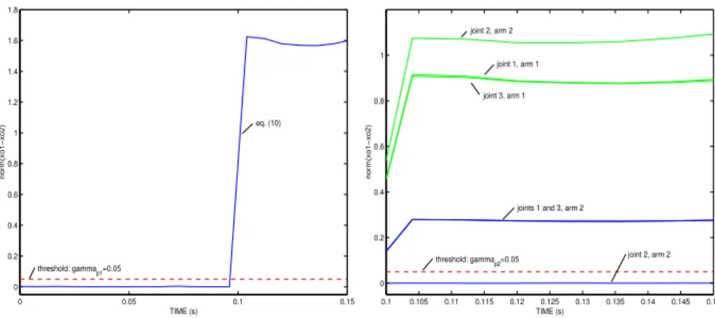
d = 3samples in the fault criteria. The parameters of the FDI system wereγp1 = γp2 = 0.05,γv1 = γv2 = 1.5,
and δj = 4×10⁻³. Figure 4 shows the detection of a JPF in a trajectory with a fault occurring at t=0.1s. The normkˆxo1(θ1)−xˆo2(θ2)k(Eq. 10) used to detect JPFs is shown on the left (Figure 4), and the normskˆxo1(θ1,ˆq1j)−
ˆ
xo2(θ2)k (Eq. 13) and kˆxo1(θ1)−ˆxo2(θ2,ˆq2j)k (Eq.
14) used to isolate JPFs is shown in the right for the joints
j= 1, . . . , n.
Table 1:Results: simulation of two three-dof arms.
Set Detected Faults Isolated Faults False
Alarms MTD(s)
1 958 (99.79%) 938 (97.71%) 0 (0%) 0.0165
2 960 (100.0%) 920 (95.83%) 0 (0%) 0.0180
3 899 (93.65%) 805 (83.85%) 0 (0%) 0.0185
4 926 (95.42%) 817 (85.10%) 0 (0%) 0.0195
Table 2:Results (faults): simulation of two three-dof arms.
Set Fault Detected Faults Isolated Faults
1 FSJF 240 (100.0%) 236 (98.33%)
1 LJF 238 (99.17%) 228 (95.00%)
1 JPF 240 (100.0%) 235 (97.92%)
1 JVF 240 (100.0%) 238 (99.17%)
2 FSJF 240 (100.0%) 238 (99.17%)
2 LJF 240 (100.0%) 209 (87.08%)
2 JPF 240 (100.0%) 238 (99.17%)
2 JVF 240 (100.0%) 236 (98.33%)
3 JPF 240 (100.0%) 238 (99.17%)
3 JVF 180 (75.00%) 098 (40.83%)
4 JPF 240 (100.0%) 236 (98.33%)
4 JVF 196 (81.67%) 135 (56.25%)
The FDI system was tested considering four trajectory sets, each one with 960 trajectories with faults occurring in dif-ferent joints and 40 without faults. The first and the second sets had the same desired trajectories, but with faults starting at 0.15 s. and 0.3 s. respectively. The four faults previously presented were simulated. In JPFs and JVFs for sets 1 and 2, the correct sensor reading were changed by random num-bers. The desired trajectories and initial time of fault of sets 3 and 4 were the same of sets 1 and 2 respectively, but the correct sensor measurements were changed by zeros in JPFs and JVFs. The results of the FDI system are summarized in table 1. The second and third columns present the number of detected faults and the number of correctly isolated faults respectively. The fourth column shows the number of false alarms in fault-free trajectories. The last column presents the Mean-Time-to-Detection (MTD): the mean time that the FDI system takes to isolate a fault after its occurrence.
The results of the FDI for each fault are summarized in table 2. The results of FSJFs and LJFs for the sets 3 and 4 are not shown (the desired trajectories in sets 3 and 4 were the same of sets 1 and 2). The number of correctly isolated JVFs was smaller in sets 3 and 4 because this fault was mistaken with LJFs. This occurred because, as the joint velocities measure-ments were changed by zeros in sets 3 and 4, JVFs generally did not present consequences in the control of the load for this controller (the load could be controlled even with the joint velocity measurements equal to zeros). This explain the small number of isolated JVFs in sets 3 and 4.
0 0.05 0.1 0.15 0
0.2 0.4 0.6 0.8 1 1.2 1.4 1.6 1.8
TIME (s)
norm(xo1−xo2)
threshold: gamma
p1=0.05
eq. (10)
0.1 0.105 0.11 0.115 0.12 0.125 0.13 0.135 0.14 0.145 0.15
0 0.2 0.4 0.6 0.8 1
TIME (s)
norm(xo1−xo2)
threshold: gammap2=0.05
joint 2, arm 2 joints 1 and 3, arm 2
joint 1, arm 1
joint 3, arm 1 joint 2, arm 2
Figure 4:FDI in a trajectory of the simulated system (three-dof planar cooperative arms) with JPF in joint 2 of arm 2 occurring att=0.1s. Left:kˆxo1(θ1)−ˆxo2(θ2)k(Eq. 10) ; Right:kˆxo1(θ1,ˆq1j)−ˆxo2(θ2)k(Eq. 13) andkˆxo1(θ1)−ˆxo2(θ2,ˆq2j)k(Eq. 14) for the joints
j= 1, . . . , n. The dashed lines show the thresholdγp2.
Table 3: Results of the FDI system: simulation (Puma560 arms).
Set Detected Faults Isolated Faults False
Alarms MTD(s)
1 718 (99.72%) 689 (95.69%) 0 (0.0%) 0.117
2 715 (99.31%) 656 (91.11%) 0 (0.0%) 0.118
manipulating a cylinder with mass equal to 2.5kg and 0.3m of length in a 3-dimensional space. The Robotics Toolbox for Matlab (Corke, 1996) was used to simulate the terms of Eq. (1) and the friction torques. The sampling period was 0.018s and measurement noise with normal distribution was added to joint positions, joint velocities, and end-effector forces.
Two MLPs were utilized: each one with 24 inputs, 49 neu-rons in the hidden layer, and 6 outputs. The MLPs were trained with 6804 patterns obtained in the simulation of 50 trajectories. The RBFN had 24 inputs and 25 outputs (12 FSJFs, 12 LJFs, and normal operation) and it was trained with 5291 patterns. The parameters of the FDI system were
d= 3samples,γp1 =γp2 = 0.01,γv1 =γv2 = 0.8, and
δj= 4×10⁻³.
The FDI system was tested considering two trajectory sets, each of them with 720 trajectories with faults and 15 with-out faults. The first and the second sets have the same de-sired trajectories but with the faults starting at 0.3s and 1.3s respectively. The four faults previously presented were sim-ulated. In JPFs and JVFs, the correct sensor measurements were changed by random numbers. The results of the FDI system are summarized in table 3.
Finally, the FDI system was applied in an actual cooperative
system with two arms UARMII (Figure 5). Each UARMII is a 3-joint, planar manipulator that floats on a thin air film on an “air table”. The two arms are equal and the longitudinal axis of each joint is parallel to the gravity force. The coop-erative system is controlled by a PC running Matlab. This is possible because the drivers for the UARMII servo board are written as Matlab mex-files. Each joint of the UARMII contains a brushless DC direct-drive motor, an encoder, and a pneumatic brake, which allows one to simulate all faults discussed here. The CMCE, which was used to simulate the cooperative system with 3-dof arms, is used to control and to monitor the actual system. The robot parameters are the same of the simulated system and the sampling period was chosen as 0.05s. The joint velocities are obtained by encoder mea-surements (the adaptive filter presented in (Wijngaard, 1996) is used), and force sensors are not used (the end-effector forces are estimated using the kinematic and dynamic mod-els).
Two MLPs were utilized to reproduce the model of the ac-tual robots: each one with 12 inputs, 37 neurons in the hidden layer, and 3 outputs. The MLPs were trained with 3250 patterns obtained in the simulation of 50 trajectories. The RBFN had 12 inputs and 13 outputs (6 FSJFs, 6 LJFs, and normal operation) and it was trained with 2506 patterns. The parameters of the FDI system were d = 4 samples,
Table 4:Results: actual system.
Set Det. Faults Is. Faults False Al. MTD(s)
1 337 (93.6%) 260 (72.2%) 1 (6.7%) 0.469
2 333 (92.5%) 247 (68.6%) 0 (0.0%) 0.419
3 325 (90.3%) 268 (74.3%) 0 (0.0%) 0.458
occurring in each joint are summarized in Table 4. Figures 6, 7, and 8 show respectively the torques of arm 1, the residuals, and the outputs of the RBFN in a trajectory with an FSJF.
The number of correctly isolated faults was smaller in the ac-tual system mainly because FSJFs were sometimes mistaken with LJFs. This occurs because sometimes the velocities of the faulty vectors were small due to the small gravitational torques at the joints. However, in these cases, even with FSJFs, the load converged to the desired positions and the fault does not present significant effects in the system. This occurred, for example, when it was not necessary to apply high torques at the faulty joint during the given trajectory.
Figure 5:Actual system: arm 1 (left); arm 2 (right).
5
CONCLUSIONS
This work presents an FDI system for cooperative manipu-lators. Four faults were considered: FSJFs, LJFs, JPFs, and JVFs. The first two are detected by ANNs: MLPs to re-produce the dynamics of the arms and an RBFN to classify the residual vector. The remaining faults are detected using the kinematic constraints of the system. Tests of the FDI system applied to simulated cooperative arms and to actual robots were presented. As the number of correctly detected faults is greater than the number of correctly isolated faults, additional tests can be done after the detection of a fault to confirm the isolated fault. If a LJF is isolated in the jointi
for example, a simple test to confirm this fault is to apply a torque in this joint and to check if the jointimoves after ap-plying the brakes in all joints. Tests to confirm the isolation of the other faults can be done in similar ways.
Figure 6:Joint torques of arm 1 in a trajectory of the actual system with FSJF in joint 1 (arm 1) occurring att=1s.
0 0.5 1 1.5
−0.1 −0.05 0 0.05 0.1
TIME (s)
RESIDUAL
Figure 7:Residuals in a trajectory of the actual system with FSJF in joint 1 (arm 1) occurring att=1s.
Acknowledgments
The authors would like to thank Marcel Bergerman for his contributions. This work was supported by FAPESP under grants 98/15732-5 and 99/10031-1.
REFERENCES
Bonitz, R. and Hsia, T. (1996). Internal force-based impedance control for cooperating manipulators,IEEE Trans. on Rob. and Aut.12: 78–89.
Figure 8: Outputs of the RBFN in the same trajectory shown in Fig. 6 (Output 1: FSJF in joint 1 of arm 1; Output 13: normal operation).
Carignan, C. R. and Akin, D. L. (1988). Cooperative control of two arms in the transport of an inertial load in zero gravity,IEEE Journal of Rob. and Aut.4(4): 414–419.
Chen, J. and Patton, R. J. (1999). Robust model-based fault diagnosis for dynamic systems, Kluwer Academic Pub-lishers.
Corke, P. (1996). A robotics toolbox for MATLAB,IEEE Robotics and Automation Magazine3(1): 24–32.
English, J. D. and Maciejewski, A. A. (1998). Fault tolerance for kinematically redundant manipulators: antecipating free-swinging joint failures, IEEE Trans. on Rob. and Aut.14(4): 566–575.
Gertler, J. (1997). A cautious look at robustness in residual generation,Proc. of the 3rd IFAC Simposium on Fault Detection, Supervision and Safety for Technical Pro-cesses, Vol. 1, pp. 133–139.
Goel, M., Maciejewski, A. A. and Balakrishnan, V. (2004). Analyzing unidentified locked-joint failures in kine-matically redundant manipulators,Journal of Robotic Systems22(1): 15–29.
Hassan, M. and Notash, L. (2004). Analysis of active joint failure in parallel robot manipulators, Journal of Me-chanical Design126(6): 959–968.
Hassan, M. and Notash, L. (2005). Design modification of parallel manipulators for optimum fault tolerance to joint jam,Mechanism and Machine Theory40(5): 559– 577.
Isermann, R. and Ball´e, P. (1997). Trends in the application of model-based fault detection and diagnosis of techi-cal processes,Control Engineering Practice5(5): 709– 719.
Koivo, A. J. and Unseren, M. A. (1991). Reduced or-der model and decoupled control architecture for two manipulators holding a rigid object, Journal of Dyn. Syst., Measurement, and Control (Trans. of the ASME) 113: 646–654.
K¨oppen-Selinger, B. and Frank, P. M. (1996). Neural net-works in model-based fault diagnosis, Proc. of 13th IFAC World Congress, pp. 67–72.
Korbicz, J. (1997). Neural networks and their application in fault detection and diagnosis,Proc. of the 3rd IFAC Simposium on Fault Detection, Supervision and Safety for Technical Processes, Vol. 1, pp. 377–382.
Looney, C. G. (1997). Pattern recognition using neural net-works, Oxford University Press.
Luh, J. Y. S. and Zheng, Y. F. (1987). Constrained re-lations between two coordinated industrial robots for robot motion control,Int. Journal of Robotic Research 6(3): 60–70.
Mangoubi, R. S. (1998). Robust estimation and failure de-tection, Springer-Verlag.
Marcu, T. and Mirea, L. (1997). Robust detection and isola-tion of process fault using neural networks,IEEE Con-trol Systems17(5): 72–79.
McIntyre, M. L., Dixon, W. E., Dawson, D. M. and Walker, I. D. (2005). Fault identification for robot manipulators, IEEE Trans. on Robotics21(5): 1028–1034.
Nahon, M. and Angeles, J. (1992). Minimization of power losses in cooperating manipulators, Journal of Dyn. Syst., Measurement, and Control (Trans. of the ASME) 114: 213–219.
Nakamura, Y. (1991). Advanced robotics: redundancy and optimization, 1st edn, Addison-Wesley Publishing Company, Inc., New York.
Naugthon, J. M., Chen, Y. C. and Jiang, J. (1996). A neural network aplication to fault diagnosis for robotic manip-ulator,Proc. of IEEE Int. Conf. on Control App., Vol. 1, pp. 988–1003.
Schneider, H. and Frank, P. M. (1996). Observer-based su-pervision and fault-detection in robots using nonlinear and fuzzy logic residual evaluation, IEEE Trans. on Control Syst. Tech.4(3): 274–282.
Sciavicco, L. and Siciliano, B. (1996). Modeling and con-trol of robot manipulators, McGraw-Hill International Editions.
Sorsa, T. and Koivo, H. N. (1993). Application of artificial neural networks in process fault diagnosis,Automatica 29(4): 843–849.
Terra, M. H. and Tin´os, R. (2001). Fault detection and iso-lation in robotic manipulators via neural networks - a comparison among three architectures for residual anal-ysis,Journal of Robotic Systems18(7): 357–374.
Tin´os, R., Terra, M. H. and Bergerman, M. (2001). Fault detection and isolation in cooperative manipulators via artificial neural networks,Proc. of IEEE Conf. on Con-trol App., pp. 988–1003.
Tin´os, R., Terra, M. H. and Ishihara, J. Y. (2006). Motion and force control of cooperative robotic manipulators with passive joints, IEEE Trans. on Control Systems Tech-nology14(4): 725–734.
Uchiyama, M. (1998). Multirobots and cooperative systems, inB. Siciliano and K. P. Valavanis (eds),Control prob-lems in robotics and automation, Springer-Verlag, Lon-don, U. K.
Vemuri, A. T. and Polycarpou, M. M. (2004). A methodol-ogy for fault diagnosis in robotic systems using neural networks,Robotica22(4): 419–438.
Visinsky, M. L., Cavallaro, J. R. and Walker, I. D. (1994). Robotic fault detection and fault tolerance: a survey, Reliability Eng. and Syst. Safety46: 139–158.
Visinsky, M. L., Cavallaro, J. R. and Walker, I. D. (1995). A dynamic fault tolerance framework for remote robots, IEEE Trans. on Rob. and Aut.11(4): 477–490.
Vukobratovic, M. and Tuneski, A. (1998). Mathematical model of multiple manipulators: cooperative compliant manipulation on dynamical environments,Mechanism and Machine Theory33: 1211–1239.
Wen, T. and Kreutz-Delgado, K. (1992). Motion and force control for multiple robotics manipulators,Automatica 28(4): 729–743.
Wijngaard, W. (1996). An adaptive filter for low frequency encoder applications,Measurement18(1): 1–7.
APPENDIX
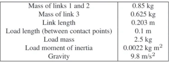
Table 5:Parameters of the simulated system (3-dof arms).
Mass of links 1 and 2 0.85 kg Mass of link 3 0.625 kg
Link length 0.203 m
Load length (between contact points) 0.1 m
Load mass 2.5 kg
Load moment of inertia 0.0022 kg m2