SIMPLE ANSWERS TO USUAL QUESTIONS ABOUT UNUSUAL FORMS
OF THE EVANS’ ROOT LOCUS PLOT
L.H.A. Monteiro
∗[email protected], [email protected]
J.J. Da Cruz
†∗Escola de Engenharia da Universidade Presbiteriana Mackenzie e Escola Polit´ecnica da Universidade de S˜ao Paulo
†Escola Polit´ecnica da Universidade de S˜ao Paulo
ABSTRACT
After a first contact with Evans’ root locus plots, in an intro-ductory course about classical control theory, students usu-ally pose questions for which the answers are not triviusu-ally found in the usual textbooks. Examples of such questions are: Can a branch intersect itself? Can two or more branches be coincident? Can a branch intersect its asymptote? In this paper devoted to helping teaching, numerical examples and an incremental property are used for answering some ques-tions about unusual forms of root loci related to closed-loop control systems. In some cases, answering to these questions can be fundamental for making a correct sketch of a root lo-cus.
KEYWORDS: feedback control, root locus method.
RESUMO
Ap´os um primeiro contato com gr´aficos de Evans de lugar das ra´ızes, num curso introdut´orio sobre teoria de controle cl´assico, os estudantes normalmente fazem perguntas para as quais as respostas n˜ao s˜ao encontradas trivialmente nos livros-textos usuais. Exemplos de tais quest˜oes s˜ao: Um ramo pode se auto-interseccionar? Dois ou mais ramos po-dem ser coincidentes? Um ramo pode interseccionar sua ass´ıntota? Neste artigo com fins did´aticos, usam-se exemplos
Artigo submetido em 31/01/2008 1a. Revis ˜ao em 26/05/2008 2a. Revis ˜ao em 13/10/2008
Aceito sob recomendac¸ ˜ao do Editor Associado Prof. Jos ´e Roberto Castilho Piqueira
num´ericos e uma propriedade incremental para responder al-gumas quest˜oes sobre formas incomuns de lugar das ra´ızes relacionadas a sistemas de controle em malha fechada. Em alguns casos, responder a essas quest˜oes pode ser fundamen-tal para fazer um esboc¸o correto de um lugar das ra´ızes.
PALAVRAS-CHAVE: controle com realimentac¸˜ao, m´etodo do lugar das ra´ızes.
1
INTRODUCTION
Analysis and design of linear time-invariant, single-input/single-output, feedback control systems can be per-formed by using the root locus method. For instance, this method can be employed for determining the lock-in range of phase-locked loops (e.g. Piqueira and Monteiro, 2006). Root locus method was introduced in 1948 by W.R. Evans (1948, 1950) in order to make possible sketching the path (in the complex plane) of the closed-loop poles of control systems, as the value of a single parameter is varied. This parameter is normally the open-loop gaink≥0. IfG(s)is the open-loop transfer function, the closed-loop poles are the roots of the characteristic equation (e.g. Ogata, 2001):
1 +kG(s) = 0 (1)
By takingG(s) ≡b(s)/a(s), wherea(s)andb(s)are real coprime polynomials of degreesnandm, respectively, then (1) can be written as:
1 + kb(s)
G(s)
q
k
Figure 1: Block diagram of a control system.
−3 −2.5 −2 −1.5 −1 −0.5 0 0.5 1 1.5 2 −2
−1.5 −1 −0.5 0 0.5 1 1.5 2
Real Axis
Imag Axis
Figure 2: Root locus forG(s) = 1/(s2+ 2s)
.
Evans derived rules that allow to sketch the loci (the branches) of the roots of equation (2) as k is varied from zero to infinity, without solving such an equation (the case
k <0is studied, for instance, by Eydgahi and Ghavamzadeh, 2001; Teixeira et alii, 2004). This sketch is based on the val-ues of the polespj ofG(s)(j = 1, ..., n), which are then
roots of the polynomiala(s); and on the zeroszj ofG(s)
(j= 1, ..., m), which are themroots of the polynomialb(s). For physically realizable systems, thenn≥m.
Evans’ rules are usually presented in an introductory subject on control systems in undergraduate engineering courses and they are simple to be applied. Some well-known rules are (e.g. Kuo, 1967; Franklin et alii, 1986; Ogata, 2001): the number of branches of the root locus is equal ton; ifn > m, then fork→ ∞there arev≡n−mbranches approaching straight-line asymptotes; branches can leave from or arrive to the real axis, and so on.
However, after seeing some examples of root locus plot, stu-dents usually ask questions that can not be easily answered
−2 −1.5 −1 −0.5 0 0.5 1 −2
−1.5 −1 −0.5 0 0.5 1 1.5
Real Axis
Imag Axis
Figure 3: Root locus forG(s) = 1/(s+ 1)3
.
with the rules presented in the course and found in the text-books. For instance: Which are the angles of departure (or arrival) of the branches leaving from (or arriving to) the real axis? Can a branch intersect itself? Can two or more branches have a common point? Can two or more branches be coincident for an open interval of values ofk? Can a branch intersect its asymptote? Here, we answer such ques-tions with numerical examples and/or arguments based on analytical expressions. These answers can be found in the literature (as cited below); however, they are barely used for sketching root loci. Here we present examples where the sketches of the corresponding root loci can not be appropri-ately made without such answers.
In the next section, an incremental property of the root locus plot is derived from a didactical block diagram. This property is employed in part of this study. The presented root loci were numerically plotted by using the software Matlab.
2
INCREMENTAL PROPERTY
Consider the feedback control system illustrated in Fig. 1 where0≤q, k <∞. The closed-loop poles are given by:
1 + (q+k)G(s) = 0 (3)
or:
1 + k b(s)
a(s) +qb(s) = 0 (4)
−7 −6 −5 −4 −3 −2 −1 0 1 2 −5
−4 −3 −2 −1 0 1 2 3 4 5
Real Axis
Imag Axis
Figure 4: Root locus forG(s) = 1/(s4+ 8s3+ 18s2+ 16s+
1).
case, the root locus plot can be determined from the zeros of
G(s)(the roots ofb(s)) and the closed-loop poles ofG(s)for
q=q1(the roots ofa(s) +q1b(s)). This result represents an
incremental property of the root locus plot: the closed-loop poles fork > k1 ≡ q1+k0is a function of the open-loop
zeros and of the closed-loop poles fork = k1. The usual
situation occurs fork1 = 0, which implies that the roots of
equation (2) depend on the roots of the polynomialsa(s)and
b(s), as Evans proved.
Incremental property, also denominated continuation prop-erty (e.g. Kuo, 1967; Pan and Chao, 1978; Franklin et alii, 1986; Paor, 2000), is an obvious consequence of the diagram shown in Fig. 1, which was not found in any control texts: the inner loop can be considered as the open-loop to draw the root locus for a varyingk >0.
3
ARRIVAL AND DEPARTURE ANGLES
The angle associated to the complex number s satisfying the equation (2) must be an odd multiple of180o, because
kG(s) =−1. Thus:
m
X
j=1
φj − n
X
j=1
θj = (2l+ 1)180o (5)
wherel = 0,±1,±2, .... The angles of the vectors from the zeroszj and the polespj to the numbersare, respectively,
φj≡arg(s−zj)andθj ≡arg(s−pj).
A breakaway point is a real roots=s1of equation (2)
oc-curring atk=k∗whererbranches (withr≥2) depart from
−2 −1.5 −1 −0.5 0 0.5 1 −2.5
−2 −1.5 −1 −0.5 0 0.5 1 1.5 2 2.5
Real Axis
Imag Axis
Figure 5: Root locus forG(s) = 1/(s4
+4s3
+8s2
+8s+3).
the real axis at s = s1 fork > k∗. A break-in point is a
real roots=s1 of equation (2) occurring atk =k∗where
rbranches (withr≥2) arrive to the real axis ats=s1for
k > k∗. In both cases, whenk = k∗, thens
1 is a root of
equation (2) with multiplicityr.
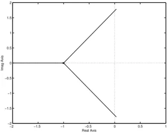
The incremental property can be used for obtaining angles of arrival and angles of departure from break-in and breakaway points, respectively. The usual example is given byG(s) = 1/(s2 + 2s)
, where the closed-loop poles are the roots of
s2+ 2s+k = 0
. Notice thats= s1 = −1is a root with
multiplicity two fork=k∗ = 1; and fork >1, both roots
become complex numbers. The departure angles from the real axis ats= s1can be determined from the closed loop
poles atk=k∗. The expression (5) reveals that these angles
are:
θj = 180o
r +j
360o
r (6)
withj= 0,1, ..., r−1. In this case,r= 2and the departure angles are90oand270o, as shown in Fig. 2.
ForG(s) = 1/(s+ 1)3
, the departure angles are60o,180o
and300o, as illustrated in Fig. 3. These angles are obtained
from expression (6) withr= 3. Observe thats=s1=−1
is the breakaway point at k = k∗ = 0, which is also the
open-loop pole with multiplicity three.
ForG(s) = 1/(s4
+8s3
+18s2
+16s+1), thens=s1=−1
is a root with multiplicity three fork=k∗= 4, as shown in
Fig. 4. The departure angles obtained from (6) are the same of the previous example, which are60o,180oand300o.
−4 −3 −2 −1 0 1 2 −8
−6 −4 −2 0 2 4 6
Real Axis
Imag Axis
Figure 6: Root locus forG(s) = (s2+ 2s+ 10)/(s5+ 9s4+
40.25s3+ 106.5s2+ 141.75s+ 67.5)
.
(1967) and Krajewski and Viaro (2007).
4
INTERSECTION AMONG BRANCHES
Breakaway and break-in points are usual examples of com-mon points acom-mong branches on the real axis. However, there can be such points also out of the real axis.
•Two or more branches can intersect at a point that does not belong to the real axis.
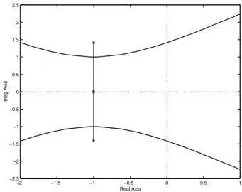
Here intersection means having a common point (a different meaning is given by Lundberg (2007)). This situation oc-curs whenever there are multiple closed-loop poles outside the real axis. For instance,G(s) = 1/(s4
+4s3
+8s2
+8s+3)
presentss = −1±ias closed-loop poles fork = 1, both poles with multiplicity two. In this example, the departure angles from these complex poles are0oand180o, as shown
in Fig. 5 (found also in Kuo (1967)), because expression (6) reduces to:
θj = j.180o (7)
withj = 0,1.
•A branch can not intersect itself.
This property is immediate since, by construction, the gaink
increases along the root locus branches. By contradiction, if such an intersection occurred there would be a point corre-sponding to two distinct values ofk.
• Two or more branches can not be coincident in an open interval of values ofk.
−4 −3 −2 −1 0 1 2
−4 −3 −2 −1 0 1 2 3
Real Axis
Imag Axis
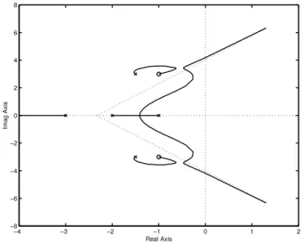
Figure 7: Root locus for G(s) = (s2 + (5/6)s +
(1/3))/(s3(s2+ 6s+ 16))
.
This is because if branches intersect at a point of the complex plane fork=k′, then they must separate following distinct angles fork = k′ +q, withq → 0+ (these angles can be
calculated by expression (6)). Consequently, these branches are no more coincident fork=k′+q.
5
INTERSECTION BETWEEN A BRANCH
AND ITS ASYMPTOTE
In Fig. 2, both branches fork > 1are coincident with the corresponding asymptotes. A similar behavior is observed in Fig. 3, where the three branches are coincident with their asymptotes fork >0. Thus, it is easy to find examples where a branch and its asymptote coincide for an open interval of values ofk.
However, it is hard to build a transfer function where this co-incidence happens at a unique point. In fact, such a behavior is possible and it is illustrated in Fig. 6, obtained forG(s) = (s2+2s+10)/(s5+9s4+40.25s3+106.5s2+141.75s+67.5)
(other examples can be found in Kuo (1967) and Ogata (2001)). Notice that two branches present a common point with the corresponding straight-line asymptotes (represented in the figure by dotted lines forming angles of60oand300o
with respect to the real axis). The third asymptote (at180o)
is coincident with its corresponding real branch fork >0.
6
HARD TO SKETCH
−4 −3 −2 −1 0 1 2 −4
−3 −2 −1 0 1 2 3 4
Real Axis
Imag Axis
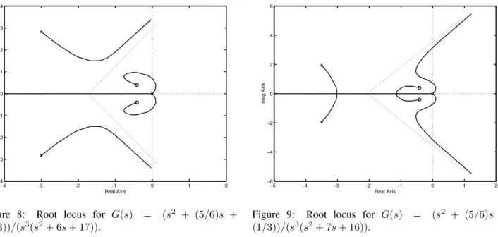
Figure 8: Root locus for G(s) = (s2 + (5/6)s +
(1/3))/(s3(s2+ 6s+ 17))
.
the real axis and without determining the arrival and depar-ture angles related to such points. In some cases, intersec-tions among branches and asymptotes should also be inves-tigated in order to perform a right sketch. For instance, take
G(s) = (s2+ (5/6)s+ (1/3))/(s3(s2+ (6 +α)s+ 16 +β)
. Fig. 7 corresponds toα = 0andβ = 0, Fig. 8 toα = 0
andβ = 1, and Fig. 9 toα= 1andβ = 0. In all cases, the departure angles from the origin (a triple pole) are60o,180o
and300o, as in Fig. 4. In Fig. 7 there are two common points
out of the real axis (in−1±i); in the other cases such points do not exist. In Figs. 7 and 8 there are neither breakaway point nor break-in point and the branches going to infinity in the right half-plane arrive from the complex poles. However, in Fig. 7 two branches intersect twice their asymptotes; in Fig. 8 such intersections do not occur. In Fig. 9 there are one breakaway point and one break-in point, the branches going to infinity in the right half-plane come from the origin, and intersections among branches and asymptotes do not happen. Observe that correct sketches of the these cases can be made only if the common points among branches out the real axis and the intersections among branches and asymptotes are cal-culated. For instance, as in Fig. 8 there is no intersection among branches and asymptotes, then the branches going to infinity in the right half-plane must arrive from the complex poles and the ones going to zeros must arrive from the origin. In Fig. 9 as such intersections do not occur either, then the branches going to infinity in the right half-plane must come from the origin (because, if not, then two branches coming from the origin should intersect the asymptotes in order to arrive in the break-in point situated at the left of the point where the asymptotes meet the real axis).
−5 −4 −3 −2 −1 0 1 2
−6 −4 −2 0 2 4 6
Real Axis
Imag Axis
Figure 9: Root locus for G(s) = (s2 + (5/6)s +
(1/3))/(s3(s2+ 7s+ 16))
.
By comparing the three last figures, it is evident that a root lo-cus plot can be drastically changed by slightly varyingG(s)
(in these cases, by slightly varying the positions of the open-loop poles and keeping unaltered the positions of the zeros).
As a “homework” we suggest to sketch the case withα= 0
andβ=−1.
7
FINAL COMMENTS
By using an incremental property (here didactically ex-plained) and/or numerical examples, we answered the ques-tions posed at the Introduction about unusual forms of root loci. The investigated features can be really useful for sketch-ing root loci, as shown in the last section. We hope that the examples as well as the reasoning presented can help root locus teaching.
The authors are partially supported by CNPq.
8
REFERENCES
Evans, W.R. (1948). Analysis of Control System, AIEE Transactions, vol. 67, pp. 547-551.
Evans, W.R. (1950). Control System Synthesis and Root Lo-cus Method,AIEE Transactions, vol. 69, pp. 66-69.
back Control of Dynamic Systems. Addison-Wesley, Read-ing, USA.
Krajewski, W., Viaro, U. (2007). Root-Locus Invariance – Exploiting Alternative Arrival and Departure Points, IEEE Control Systems Magazine, vol. 27(1), pp. 36-43.
Kuo, B.C. (1967).Automatic Control Systems, Prentice-Hall, Englewood-Cliffs, USA.
Lundberg, K.H. (2007). Classical Crossroads,IEEE Control Systems Magazine, vol. 27(6), pp. 20-21.
Ogata, K. (2001). Modern Control Engineering, Prentice-Hall, New York, USA.
Pan, C.T., Chao, K.S. (1978). A Computer-Aided Root Lo-cus Method,IEEE Transactions on Automatic Control, vol. 23, pp. 856-860.
Paor, A.M. (2000). The Root Locus Method: Famous Curves, Control Designs and Non-control Applications, In-ternational Journal of Electrical Engineering Education, vol. 37, pp. 344-356.
Piqueira, J.R.C., Monteiro, L.H.A. (2006). All-Pole Phase-Locked Loops: Calculating Lock-In Range by Using Evan’s Root-Locus,International Journal of Control, vol. 79, pp. 822-829.