Numerical Study on the Influence of Tip Clearance

UNIVERSIDADE DA BEIRA INTERIOR

Engenharia

Numerical Study on the Influence of Tip

Clearance

Patrick Leonard O’Neill

Dissertação para obtenção do Grau de Mestre em

Engenharia Aeronáutica

(Ciclo de estudos integrado)

Orientador: Prof. Doutor Francisco Miguel Ribeiro Proença Brójo

iii

v

Acknowledgments

I would first like to thank my thesis advisor, Professor Doutor Francisco Miguel Ribeiro Proença Brójo. The door to Prof. Brójo’s office was always open whenever I ran into a trouble spot or had a question about my research and writing. He always allowed this paper to be my own work, but steered me in the right direction whenever he thought I might need it.

I would also like to thank all of my friends for their support and friendship over these years. The countless hours of fun and comradery were the most a friend could ask for.

Finally, but most importantly, I wish to thank my Mother Luísa, my Father Patrick and my sister Kelly for their patience, assistance, support and faith in me throughout my years of study and through the process of researching and writing this thesis. This accomplishment would not have been possible without them. Thank you.

Patrick O’Neill Covilhã, June 2017

vii

Resumo

Devido a um aumento constante dos custos e ao continuado aumento na procura por parte de clientes, as companhias aéreas investigam novas tecnologias como forma de reduzir custos operacionais, como os custos de combustível. Com tais objectivos em mente, a NASA e outras organizações estão a estudar e a testar novas configurações de turbinas a gás para determinar se poderá ser uma solução viável num futuro próximo.

São realizadas várias simulações numéricas para uma pá de um compressor axial, de forma a verificar a influência da razão de pressão total e velocidade de escoamento na diferença entre a folga na ponta e a ausência de folga no topo da pá.

As simulações de CFD foram realizadas utilizando o FLUENT onde é possível determinar as condições de entrada e de saída da experiência bem como as condições de fronteira que permitem colocar o problema corretamente para que seja obtida uma solução realista.

Nesta tese foram estudados dois modelos diferentes, No-Tip Gap (sem espaçamento) e Tip Gap (com espaçamento). Cada um destes modelos foi depois simulado com três diferentes velocidades de rotação da pá para que seja possível determinar qual o seu impacto e perceber qual seria mais benéfica em projectos futuros.

Após a realização das simulações foi possível determinar que existe uma pressão maior no modelo No-Tip Gap. Esta pressão superior pode ser explicada analisando a área de superfície da pá em ambos os modelos. No modelo No-Tip Gap a pá do compressor ocupa toda a área desde a raiz até à nacele do motor, logo a sua área será superior, transferindo mais trabalho e consequentemente criando uma maior pressão à saída do que o modelo Tip Gap.

No que toca à velocidade, os resultados foram o inverso. Uma maior velocidade foi obtida quando simulado o modelo Tip Gap. Esta maior velocidade pode ser explicada devido à existência do espaçamento na ponta da pá. O escoamento passando por este espaço não entra em contacto com a pá, não reduzindo a sua velocidade, resultando numa velocidade de saída mais elevada.

Palavras-chave

ix

Abstract

Due to a constant rise in costs and a continuous demand for travel from customers, airlines look to new technologies as a way of potentially reducing operational costs, such as fuel costs. With such objectives in mind, NASA and other organizations are studying and experimenting new configurations of gas turbines to determine if this could be a viable solution for the near future.

Several simulations are run for an axial compressor blade in order to verify the influence in total pressure ratio and flow velocity between the No-Tip Gap model and the Tip Gap model. This will determine the impact of tip clearance on the aforementioned parameters.

The CFD simulations will be carried out using FLUENT where it is possible to determine the inlet and outlet conditions of the experiment as well as other boundary conditions to properly present the problem and a realistic solution.

In this study two distinct models will be simulated, No-Tip Gap and Tip Gap, each at three different rotational speeds to simulate the impact for different velocities of blade rotation and determine which model would be more beneficial for future turbines.

It was concluded that the pressure along the blade using the No-Tip Gap model was higher when compared to the Tip Gap model. This could be explained by simply analysing the surface area of the blade. Being that the blade occupies the area up to the engine casing it will have a greater surface area, hence, transferring more work and having higher pressure at the compressor exit.

As for the velocity, the results were reversed, meaning that a higher velocity of flow was found when using the Tip Gap model. The explanation for this higher speed could be the existence of a tip clearance, allowing the flow to pass through this area with no contact with the blade and therefore not reducing the speed of the airflow resulting in a higher outlet velocity.

Keywords

xi

Contents

1 Introduction ... 1

1.1 Motivation ... 1

1.2 Objectives ... 1

1.3 Contextualization ... 1

1.4 State of the Art: Transonic Axial Compressors ... 3

1.4.1 Blade Profile Studies ... 4

1.4.2 Three-Dimensional Shaped Bladings ... 5

1.4.3 Concluding Remarks... 8

2 Literature Review ... 9

2.1 What is a gas turbine? ... 9

2.2 Advantages and Disadvantages of gas turbines ... 9

2.2.1 Advantages ... 9

2.2.2 Disadvantages ... 9

2.3 Gas turbine cycle ... 10

2.4 Adiabatic efficiency ... 12

2.5 Total pressure ratio ... 13

2.6 Stagnation Pressure ... 13

2.7 Convergent and divergent ducts ... 13

2.8 Engine Sections ... 14

2.8.1 Inlet ... 15

2.8.2 Compressor ... 15

2.8.3 Diffuser ... 16

2.8.4 Combustor ... 16

2.8.5 Turbine ... 16

2.8.6 Propelling nozzle ... 17

2.9 Efficiency and performance ... 17

2.10 Atmospheric conditions ... 18

2.11 Compressor stall and compressor surge ... 18

2.11.1 Causes of Compressor Stall ... 20

2.11.2 Rotating Stall ... 20

2.11.3 Axi-Symmetric Stall ... 20

2.12 Tip Clearance ... 21

xii

2.14 Computational Fluid Dynamics ... 22

3 Rotor 67 ... 25

4 Methodology ... 27

4.1 Geometry ... 27

4.2 Mesh ... 27

4.3 Setup ... 30

4.3.1 Standard Initialization ... 34

4.3.2 Hybrid Initialization ... 35

4.4 Solution ... 35

4.5 Results ... 36

5 Experimental Configuration ... 37

5.1 Geometry ... 37

5.2 Mesh ... 38

5.2.1 No-Tip Gap ... 39

5.2.2 Tip Gap ... 40

5.3 Setup ... 41

5.3.1 No-Tip Gap ... 41

5.3.2 Tip Gap ... 45

5.4 Solution ... 45

5.5 Results ... 46

6 Results ... 47

6.1 Grid-Independence ... 48

6.2 No-Tip Gap ... 49

6.3 Tip Gap ... 56

6.4 Comparison between both models ... 63

7 Conclusion and Future Works ... 65

7.1 Conclusion ... 65

7.2 Future Works ... 66

xiii

Figure List

Figure 1 - Types of Gas Turbines Figure 2 – Axial Compressor

Figure 3 – Blade deformation (left) and Mach number contours (right) before and after optimization (Burgurubu et al., 2004)

Figure 4 - Blade axial curvature impact on shock, suction side boundary layer and blade wake development (Benini & Biollo, 2008)

Figure 5 - Baseline (left) and optimized (right) Mach number distribution at 90% span (Ahn & Kim, 2002)

Figure 6 - Gas Turbine Figure 7 - Two stroke engine Figure 8– Ideal Brayton Cycle

Figure 9 - Ideal Brayton Cycle vs Actual Brayton Cycle Figure 10 - Convergent (left) and Divergent (right) ducts Figure 11 – Engine cross section

Figure 12 - Compressor surge margin Figure 13 - Schematic view of tip clearance Figure 14 - Tip-leakage flow

Figure 15 - Computational Fluid Dynamics simulation

Figure 16 - Differential control volume considered for derivation of conservative equations Figure 17 - NASA Rotor 67

Figure 18 - Vectors used to compute Orthogonal Quality for a face Figure 19 - Calculating the Aspect Ratio

Figure 20 - Grid check tools Figure 21 - Model Dialog Box Figure 22 - Solution Methods Panel Figure 23 - Solution Controls Panel

Figure 24 - Diverging Solution ("Blowing up")

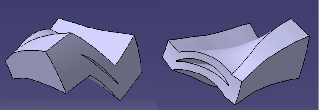
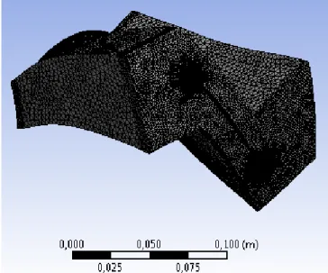
Figure 25 - Geometry of No-Tip Gap from two different views Figure 26 - Geometry of Tip Gap from two different points of view Figure 27 - Mesh 1 (with the refinements)

xiv

Figure 29 - Mesh 3 (after being refined) Figure 30 - Tip Gap Mesh (after refinements) Figure 31 - Mass Flow Inlet

Figure 32 - Moving Wall Boundary Conditions Figure 33 - Solution Methods

Figure 34 - Surface Monitor dialog box

Figure 35 - Stagnation Pressure at Outlet [Pa] vs Number of Nodes

Figure 36 – RPM 100%: Contours of total pressure (Pascal) along the different planes Figure 37– RPM 100%: Contours of velocity magnitude (m/s) along the different planes Figure 38 – RPM 100%: Contours of total pressure (Pascal) at 75%

Figure 39 – RPM 100%: Contours of total pressure (Pascal) at 25% Figure 40 - RPM 100%: Contours of velocity magnitude (m/s) at 75% Figure 41 - RPM 100%: Contours of velocity magnitude (m/s) at 25% Figure 42 - RPM 90%: Contours of total pressure (Pascal) at 75% Figure 43 - RPM 90%: Contours of total pressure (Pascal) at 25% Figure 44 - RPM 80%: Contours of total pressure (Pascal) at 75% Figure 45 - RPM 80%: Contours of total pressure (Pascal) at 25% Figure 46 - Velocity Magnitude (m/s) represented in vector form

Figure 47 - Velocity Magnitude (m/s) represented in vector form. Close up on Leading Edge Figure 48 - RPM 100%: Contours of total pressure (Pascal) along the different planes Figure 49 - RPM 100%: Contours of velocity magnitude (m/s) along the different planes Figure 50 - RPM 100%: Contours of total pressure (Pascal) at 25%

Figure 51 - RPM 100%: Contours of total pressure (Pascal) at 75% Figure 52 - RPM 100%: Contours of velocity magnitude (m/s) at 25% Figure 53 - RPM 100%: Contours of velocity magnitude (m/s) at 75% Figure 54 - RPM 90%: Contours of total pressure (Pascal) at 75% Figure 55 - RPM 90%: Contours of total pressure (Pascal) at 25% Figure 56 - RPM 90%: Contours of velocity magnitude (m/s) at 75% Figure 57 - RPM 90%: Contours of velocity magnitude (m/s) at 25% Figure 58 - RPM 80%: Contours of total pressure (Pascal) at 75% Figure 59 - RPM 80%: Contours of total pressure (Pascal) at 25% Figure 60 - RPM 80%: Contours of velocity magnitude (m/s) at 75%

xv

Figure 61 - RPM 80%: Contours of velocity magnitude (m/s) at 25%

Figure 62 - Velocity Magnitude (m/s) represented in vector form

xvii

Table List

Table 1 - Orthogonal Quality mesh metrics spectrum Table 2 - Skewness values and corresponding cell quality Table 3 – Average Value of Mesh Quality for Different Meshes

Table 4 – Stagnation Pressure at Outlet, P2, and Number of Nodes for different mesh refinements

Table 5 - Variation of Entropy at different RPM Table 6 - Area-weighted average of .

Table 7 - Outlet Mach number

Table 8 - Variation of Entropy at different RPM Table 9 - Area-weighted average of .

xix

Nomenclature

SFC Specific Fuel Consumption

NASA National Aeronautics and Space Administration

ANSYS Analysis System

CFD Computational Fluid Dynamics

CAD Computer-Aided Design

3D Three Dimensional

Y-plus

R Gas Constant

Entropy variation

P1 Inlet total pressure

P2 Outlet total pressure

c Speed of sound R Gas Constant k Adiabatic index T Absolute temperature M Mach number u Flow speed

1

Chapter 1

1 Introduction

1.1 Motivation

Gas turbines have a strong impact on human life since its introduction during the twentieth century. They have been widely used mainly for power generation and later on in aircraft propulsion.

Gas turbine engines for commercial and military applications have dramatically evolved over the last half century through the constant pursuit of better specific fuel consumption (SFC), lower noise, lower emissions and higher thrust-to-weight ratio, to name a few, all while maintaining affordability and reliability.

Focusing on the design of gas turbines, aerodynamic features, structural integrity and vibration aspects, cooling and environmental effects are subject of active research and development to achieve maximum efficiency and performance with the least amount of noise and pollution.

1.2 Objectives

The main goal of this study is to analyse the effect of a spacing, or lack thereof, between the tip of a compressor blade and the engine casing. The gas turbine used was the NASA Rotor 67. To fully understand the possible advantages of each configuration, a study on the influence of tip clearance was conducted with total pressure ratio and flow velocity being the parameters analysed.

1.3 Contextualization

To move an airplane through the air a propulsion system is needed to generate thrust. The most widely used form of propulsion system for modern aircraft is the gas turbine engine. Gas turbines exist in different forms and are used in different ways, each with its own advantages and disadvantages. Some of these altered type of gas turbines are mentioned and analysed next.

2

Figure 1 - Types of Gas Turbines (Adapted from NASA [16])

While the engines are not the same, they share some parts in common. Figure 1 shows different engines and their components. All these engines have a combustion chamber (red), a compressor (blue), a turbine (purple) and an inlet and a nozzle (grey). The compressor, combustion chamber and turbine are called the core of the engine since all gas turbines have these components. The gas is passed through a hot nozzle to produce thrust for the turbojet, while it is used to drive the turbine (green) of the turbofan and turboprop engines. Because the compressor and turbine are connected by a central shaft and rotate together, this group of parts is called turbomachinery.

Turbomachinery plays a very important role in the industry, in the energy supply and in terms of mobility as well. Looking at it through an engineering perspective its applications can be divided into governing physics: incompressible and compressible flows.

Turbomachines that are ruled by compressible flows are designed to create a big pressure differential. The best example is the gas turbine cycle used in aircraft and automobiles: air flows through compressors, combustors and turbines.

The flow features are complicated and may be divided into compressor and turbine aerodynamics in gas turbines. Compressor aerodynamic design is challenging due to stability, especially when the maximum efficiency is within the surge margin. On the other hand, turbine aerodynamics also present a challenge due to high inlet gas temperature, secondary flow, separation and transonic flow and their interactions.

Flow can also occur in three different regimes: subsonic, transonic and supersonic. In this thesis only subsonic and transonic flow will be addressed. Transonic regime refers to the condition in which a range of velocities of airflow exist surrounding and flowing past an airfoil, or in this case a compressor blade, that are concurrently below, at and above the speed of sound in the range of Mach 0.8 to 1.2 at sea level. Subsonic flows have speeds of 0.3 to 0.8 Mach.

3

1.4 State of the Art: Transonic Axial Compressors

Transonic axial flow compressors are today widely used in aircraft engines to obtain maximum pressure ratios per single-stage. High stage pressure ratios are important because they make it possible to reduce engine size and weight and, therefore, investment and operational costs. Performance of transonic compressors has today reached a high level, unthought-of half a century ago, but engine manufacturers are oriented towards increasing it further. A small increment in efficiency, for example, can result in huge saving in fuel costs and determine a key factor for product success. Another major aim is the improvement of rotor stability towards near stall conditions, resulting in a wider working range.

A considerable contribution for new developments and designs was the progress made in the field of optical measurement techniques and computational methods. This led to a better understanding of the loss in mechanisms of supersonic relative flows in different compressors.

A closer look at the current trend in design parameters for axial flow transonic compressors shows that, especially in civil aircraft engines, the relative flow tip Mach number of the rotor is limited to maintain high efficiencies. A typical value for the rotor inlet relative flow at the tip is approximately Mach 1.3. The continuous progress of aerodynamics has been focused on the increase in efficiency and pressure ratio and the improvement in off-design behaviour at roughly the same level of the inlet relative Mach number. Today’s high efficiency transonic axial flow compressors give a total pressure ratio in the order of 1.7-1.8 per stage, realized by combining high rotor speeds and high stage loadings.

The flow field that develops inside a transonic compressor rotor is extremely complex and presents many challenges to compressor designers, who must deal with several and concurring flow features such as shock waves, intense secondary flows and shock/boundary layer interaction all of which induce energy losses and efficiency reduction. Particularly detrimental is the interaction with the tip clearance flow at the outer span of the rotor, where compressors generally show the higher entropy production.[1]

4

All compressors have different operating points. Two of these points are peak (best performance) or near-stall (almost coming to a stop, stall would mean an actual stop of the engine). As the compressor moves from peak to near-stall operation, the blade loading increases and the flow structures become stronger and more unsteady. The tip leakage vortex can breakdown interacting with the passage shock wave, leading not only to a large blockage effect at the tip but also to a self-sustaining flow oscillation in the rotor.

1.4.1 Blade Profile Studies

For relative inlet Mach numbers in the order of 1.3 and higher, the most important design intent is to reduce the Mach number in front of the passage shock. This is the primary objective and it is important due to the strongly rising pressure losses with increasing pre-shock Mach number, and because of the increasing pressure due to pre-shock/boundary layer interaction.

Besides inducing energy losses, the presence of a shockwave can make transonic compressors particularly sensitive to variations in blade section design. In 1996, Wadia & Copenhaver [2], investigated the cascade throat area, internal contraction and trailing edge effective amber on compressor performance and discovered that through small changes in meanline angles, and consequently in the airfoil shape, significantly affect the performance of transonic blade rows.

One of the most important airfoil design parameters affecting the aerodynamics of transonic bladings is the chordwise location of maximum thickness. In 1993, Wadia & Law [3], ran a numerical and experimental evaluation of two different low aspect ratio rotors, having the location of maximum thickness at 55% and 40% of the chord length. The concluded that the more aft (towards the back) position is preferred for the best high speed performance. This is because the better performance was associated with the lower shock front losses with the finer section that results when the location of maximum thickness is moved aft.

Not only the maximum thickness but also the airfoil thickness has been shown to have significant impact in the performance of transonic rotors. This was shown by Suder et al. in 1995 [4], where a 0.025mm thick coating was applied on the rotor blades resulting in an increase in 10% of the leading edge thickness at the hub and 20% at the tip. The coating applied resembled that of bare metal blade finish, meaning it did not increase the roughness of the blade except for the tip, which increased due to impact damage. This coating resulted in a 4% pressure ratio drop when it was operating near design mass flow. Adiabatic efficiency was also tested at design speed and shown to, at constant pressure, drop anywhere from 3% to 6%.

Recently, the development of optimization tools coupled with accurate CFD (Computational Fluid Dynamics) codes has improved the turbomachinery design process

5

significantly in terms of efficiency and availability. The application of this technology has allowed for a fully three-dimensional approach which can lead to optimal blade geometries in terms of aerodynamic conditions as well as off-design operating conditions. This is an important development because slight changes in airfoil design can have great impact in the performance of the blade. This tool allows for a detailed study of small variations and possible effects on performance without spending money on production of the airfoils.

Blade deformation obtained in a quasi 3D numerical optimization process of a transonic compressor blade section along with relative Mach number contours before and after the optimization was studied by Burguburu et al. in 2004. [5]

Figure 3 - Blade deformation (left) and Mach number contours (right) before and after optimization (Burgurubu et al., 2004 [5])

Figure 3 shows the results of the experiment. It can be seen that there was no difference in the inlet flow field after the optimization but the flow field structure in the duct is different. The negative curvature of the blade upstream of the shock led to the reduction of the upstream relative Mach number from 1.4 to 1.2. With this curvature change, the velocity slowdown is more noticeable. Instead of creating a normal shock, the new curvature created two different, low intensity, shocks. This resulted in an increase in 1.75% of blade efficiency without changing the chocking mass flow.

1.4.2 Three-Dimensional Shaped Bladings

The flow field in a compressor is not only influenced by the two-dimensional airfoil geometry. The three-dimensional shape of the blade is very important, especially because of the interference between optimizations of shock structures and secondary flows.

Denton and Xu, in 2002 [6], conducted a numerical investigation on the aerodynamics of 3D shaped blades in transonic compressor rotors. It showed the possibility of having a better stall margin with forward sweep (upstream movement of blade sections along the local chord direction, especially at outer span region), while maintaining a high efficiency over a wider range. This seems to be a consensus conclusion as it was also confirmed by other researchers.

6

Numerical and experimental analyses were carried out by Hah et al., 1998 [7], to evaluate the performance of a conventional unswept rotor, a forward swept rotor and an aft swept rotor. The results showed that the forward swept rotor had a higher peak efficiency as well as a larger stall margin when compared to the unswept rotor. The aft swept rotor had a similar peak efficiency but a considerably smaller stall margin. Detailed analyses of the measured and calculated flow fields indicated there were two mechanisms that were mainly responsible for the difference in aerodynamic performance of the three rotors. The first mechanism was a change in radial shape of the passage shock near the casing, caused by the enwall effect, and the second was the radial migration of the low momentum fluid to the blade tip region. A parallel investigation by Wadia et al., in 1998 [8], obtained similar results, which identified the reduced shock/boundary layer interaction, resulting from a reduced axial flow diffusion, as the prime contributor to the enhanced performance with the forward swept rotor.

A more recent numerical work by Benini & Biollo in 2008 [9], gave a different point of view on the impact of the blade curvature in transonic compressor rotors, showing that the movement of the blade section in the axial direction influence the internal flow field. This study showed that the axial curvature of the blade helps influence the shape of the shock in the meridional plane, inducing the shock to assume the meridional curvature of the blade leading edge as shown in Figure 4.

7

Figure 4 - Blade axial curvature impact on shock, suction side boundary layer and blade wake development (Benini & Biollo, 2008 [9])

It was also concluded that a considerable impact on the radial outward migration of fluid particles which takes place inside the blade suction boundary layer after the interaction with the shock has been confirmed. A reduction in the strength of this flow was predicted when the blade is curved downstream and an increment when the blade was curved upstream. This type of flow is harmful because it causes an obstruction to the boundary layer development in the streamwise direction, leading to a thickening of the blade wakes. A reduction of the flows strength helped to reduce the generation of entropy which in turn helps reduce the aerodynamic losses associated with the blade wake development.

The same research partnership, Benini & Biollo, in 2008 [10], investigated the aerodynamic effects induced by the blade curvatures of the NASA Rotor 37. It was concluded that, when curvature is applied towards the direction of the rotation of the rotor, the blade-to-blade shock tends to move further downstream, becoming more oblique to the incoming flow. This results in a decrease in aerodynamic shock losses and entropy generation. In some cases it was possible to see an increase of over 1% in peak efficiency, when at design speed. In 2002, Ahn & Kim [11], obtained similar results after the application of a numerical

8

optimization algorithm. Figure 5 shows the predicted impact of the optimized design of Rotor 37 on the blade-to-blade Mach number.

Figure 5 - Baseline (left) and optimized (right) Mach number distribution at 90% span (Ahn & Kim, 2002 [11])

1.4.3 Concluding Remarks

Transonic compressors are the state-of-the-art in the compression system in today’s military and civil aircraft’s engines. Their capability of providing high pressure ratios and ability to maintain incredibly high efficiencies make them preferable to subsonic, which have low pressure ratios, and supersonic, which have low efficiencies, solutions.

The investigations made throughout the last decades have greatly improved parameters such as efficiency and pressure ratios, and therefore the success of axial compressors. Progress made in optical measurement techniques and the development and innovation of computational methods led to a better understanding of loss mechanisms associated with supersonic flow, allowing for a significant aerodynamic and industrial diffusion.

There is still room for further improvement and new solutions to be developed in the near future. This can range from highly effective stall/surge control systems to higher pressure ratio configurations or even completely new and innovative advance working principles.

9

Chapter 2

2 Literature Review

2.1 What is a gas turbine?

A gas turbine is an internal combustion engine that uses air as the working fluid. The engine extracts chemical energy from fuel and converts it into mechanical energy using the energy of the working fluid (in this case, air) to drive the engine and/or propeller, which, in turn, make the aircraft move forward.

Figure 6 - Gas Turbine (Adapted from Computational Flow Physics Laboratory [24])

2.2 Advantages and Disadvantages of gas turbines

All the existent turbomachinery in the world have advantages due to technological advances, which are coupled with some disadvantages. Gas turbines are no exception.

2.2.1 Advantages

 Very high power-to-weight ratio

 Smaller than most engines of the same power rating

 Low vibration produced due to a smoother rotation of the main shaft

 Maintenance costs are low because there are few moving parts, resulting in higher reliability over its service life

 Run on a variety of fuels

 Very low toxic emissions of CO and HC due to an excess of air, complete combustion and no suppression of the flame

2.2.2 Disadvantages

 Core engine costs can be high because of the use of exotic materials  Less efficient at idle speeds when compared to other kinds of engines  Long start-up time

10

2.3 Gas turbine cycle

The principle of the airplane turbine engine is identical to any and all engines that extract energy from chemical fuel. There are four basic steps for any internal combustion engine, which are:

1. Intake of air (possibly fuel as well)

2. Compression of the air (possibly fuel as well)

3. Combustion, where fuel is injected and burned to convert the stored energy 4. Expansion and exhaust, where the converted energy is used

In the case of a piston engine, for example a car engine, all these steps occur in the same place (cylinder head) but at different times as the piston goes up and down. This can be a four-stroke or two-stroke engine, the principle is the same in both cases, only the time at which they happen changes because it’s not possible to perform all 4 steps at different times with a two-stroke engine.

In a two-stroke engine, the mixture of air and fuel is drawn into the crankcase by vacuum through the poppet intake valve. This occurs during the upstroke motion of the piston. During the downward stroke, the poppet valve is forced shut by the increase in pressure of the crankcase. The mixture is then compressed in the crankcase for the remainder of the downward stroke. Towards the end of the stroke, the piston exposes the intake port, allowing the compressed fuel and air mixture to enter the crankcase to escape around the piston and into the main cylinder. This expels the exhaust gases out the exhaust port, normally located on the opposite side of the cylinder. With this forcing out of the exhaust gases there is usually some fresh mixture also expelled. The piston then rises, driven by flywheel momentum, and compresses the fuel mixture. At the same time, another intake stroke is happening beneath the piston. At the top of the stroke, the spark plug ignites the mixture. The burning fuel expands, driving the piston downward, to complete the cycle. At the same time this happens, another crankcase compression stroke is happening beneath the piston.

11

In an ideal world, a gas turbine would undergo four thermodynamic processes: isentropic (or adiabatic, meaning work transfers are frictionless) compression, isobaric (constant pressure) combustion, an isentropic expansion through the turbine followed by another isobaric process, a heat rejection. These four processes together make up the Brayton cycle. In Figure 8 it is possible to see the cycle graphically, where q is heat, T is temperature, p is pressure, s is entropy and v is volume.

Figure 8– Ideal Brayton Cycle (Adapted from Wikipedia [26])

In a real gas turbine, mechanical energy is changed irreversibly (due to internal friction and turbulence) into a pressure and thermal energy when the gas is compressed. Heat is added in the combustion chamber and the specific volume of gas increases, accompanied by a slight loss in pressure. During expansion through the stator and rotor passages in the turbine, irreversible energy transformation occurs once again. Fresh air is taken in replacing the heat rejection. The comparison between an ideal and actual Brayton cycle can be seen in Figure 9.

Figure 9 - Ideal Brayton Cycle vs Actual Brayton Cycle (Adapted from NASA [27])

In a turbine engine, however, these same four steps occur at the same time but in different places. Because of this fundamental difference, the turbine has engine sections named:

12

1. Inlet section 2. Compressor section 3. Combustion section 4. Turbine section

The turbine section of the turbine has the task of producing usable output shaft power to drive the propeller. In addition, it must also provide power to drive the compressor and all engine accessories. It does this by expanding the high temperature, pressure and velocity gas and converting the gaseous energy to mechanical energy in the form of shaft power.

A large mass of air must be supplied to the turbine in order to produce the necessary power. This mass of air is supplied by the compressor, which draws the air into the engine and squeezes it to provide high-pressure air to the turbine. The compressor accomplishes this by converting mechanical energy from the turbine to gaseous energy in the form of pressure and temperature.

If the compressor and turbine were 100% efficient, the compressor would supply all the air needed by the turbine and the turbine would provide the necessary power to drive the compressor. In this case, a perpetual motion machine would exist. However, in a real world, frictional losses and mechanical system inefficiencies do not allow a perpetual motion machine to operate, as it would violate the first law of thermodynamics: the law of conservation of energy, because it would mean that the machine would be able to operate without an energy input (the total energy of an isolated system is constant; energy can be transformed from one form to another, but cannot be created or destroyed). Additional energy must be added to the air to accommodate for these losses. Power output is also desired from the engine (beyond just the energy needed to drive the compressor) so even more energy must be added.

Energy addition to the system is accomplished in the combustor. Chemical energy in the form of fuel, as it burns, is converted to gaseous energy in the form of high temperatures and high velocity as the air passes through the combustor. The gaseous energy is converted back to mechanical energy in the turbine, providing power to drive the compressor and the output shaft.

2.4 Adiabatic efficiency

Adiabatic efficiency is defined as the ratio of work output for an ideal isentropic compression process to the work input to develop the required head. It can be calculated using the following formula:

13

where k is the ratio of specific heats, and are the inlet and outlet pressures, respectively. and are outlet temperature and inlet temperature, accordingly.

2.5 Total pressure ratio

Total pressure ratio is defined as a ratio of the flow pressure after exiting the compressor to the pressure of the flow that entered the compressor. It can be obtained numerically using:

where and are inlet pressure and outlet pressure, respectively.

2.6 Stagnation Pressure

For a process with

, where Q is heat and W is work, the stagnation enthalpy,

and hence the stagnation temperature, is constant. In this situation, the stagnation pressure is

related directly to the entropy as,

where, represents the variation of entropy, is the gas constant and and are the inlet and outlet pressures, respectively.

2.7 Convergent and divergent ducts

Divergent ducts function on the principle that energy is not added or taken away, but where the gaseous energy is being converted from velocity to pressure and temperature. There is a velocity decrease as the air flows from a small inlet to a larger outlet. As velocity decreases, impact pressure also decreases. Since no energy is added or subtracted from the system, total pressure for the air remains constant and static pressure increases. One way of understanding this is that the impact pressure is converted to static pressure; therefore, a static pressure rise is noticed as the air flows through a divergent duct and is compressed. A temperature rise is also detected since compression is a heating process.

The convergent duct operates in an opposite manner to the divergent duct. Energy is neither being taken nor added to the system, but the gaseous energy is being converted from

14

pressure and temperature to velocity. There is a velocity increase as the air flows from a larger inlet to a smaller outlet. As the velocity increases, impact pressure also increases. Since no energy is added or taken away from the system, total pressure remains the same and static pressure decreases because it is converted to impact pressure; thus, a static pressure decrease is seen as air flows through a convergent duct and goes through expansion. A temperature drop is normally associated with any expansion process.

Figure 10 - Convergent (left) and Divergent (right) duct (Adapted from Model Aircraft [28])

2.8 Engine Sections

As mentioned before the engine has a number of different sections.

Figure 11 - Engine cross section (Adapted from Helicopter Page [29])

Each section will now be described in greater detail, namely: 1. Inlet 2. Compressor 3. Diffuser 4. Combustor 5. Turbine 6. Propelling Nozzle

15

2.8.1 Inlet

The air inlet duct must provide clean and unrestricted airflow to the engine. Clean and undisturbed inlet airflow extends engine life by preventing damaging processes such as erosion and corrosion.

When designing the inlet system for the airflow several conditions need to be taken into account. These conditions are mostly atmospheric. Atmospheric conditions such as dust (over deserts mostly), salt (coastal areas and flights over large bodies of salt water), industrial pollution, foreign objects (birds, bolts and nuts) and temperature (icing) must be studied and the design of the inlet system should try to minimize their impact and prolong the engine’s lifespan. Fairings should be installed between the engine air inlet housing and the inlet duct to ensure minimum airflow loss to the engine at all airflow conditions.

2.8.2 Compressor

The compressor is responsible for providing the turbine with all the air it needs in the most efficient manner possible. In addition to this, it must supply the air at high static pressures.

In an axial flow compressor, each stage incrementally boosts the pressure from the previous stage. A single stage of compression consists of a set of rotor blades attached to a rotating disk, followed by stator vanes attached to a stationary ring. The flow area between the compressor blades is slightly divergent. The flow area between the compressor vanes is also divergent, but more so than for the blades.

In general terms, the compressor rotor blades convert mechanical energy into kinetic energy. This energy conversion greatly increases total pressure. Most of the increase is in the form of velocity, with a small increase in static pressure due to the divergence of the blade flow paths.

The efficiency of a compressor is primarily determined by the smoothness of the airflow. During the design stage, every effort is made to keep the air flowing smoothly through the compressor to minimize airflow losses due to friction and turbulence. This is a difficult task since the air is forced to flow into ever-higher pressure areas.

Air has the natural tendency to flow towards low-pressure areas. If the air was allowed to flow “backwards” into lower pressure zones, the efficiency of the compressor would decrease tremendously, as the energy used to increase the pressure of the air would be wasted. To prevent this from happening, seals are incorporated at the base of each row of vanes to prevent air leakage. In addition to that, the tip clearances of the rotating blades are also kept at a minimum using a coating on the inner surface of the compressor case.

16

All components used in the flow path of the compressor are shaped in the form of airfoils to maintain the smoothest airflow possible. Just as is the case for the wings of an airplane, the angle at which the air flows across the airfoils is critical to performance. The blades and vanes of the compressor are positioned at optimum angles to achieve the most efficient airflow at the compressor’s maximum rated speed.

2.8.3 Diffuser

Air leaves the compressor through exit guide vanes, which convert the radial component of the air flow out of the compressor to straight-line flow. The air then enters the diffusers section of the engine, characterized by a very divergent duct. The primary function of the diffuser structure is purely aerodynamic. The divergent duct shape converts most of the air’s velocity into static pressure. Thus, the highest pressure and lowest velocity in the entire engine is at the point of diffuser discharge and combustor outlet.

In addition to critical aerodynamic functions, the diffuser also provides:  Engine structural support, including engine mounting to the nacelle  Support for the rear compressor bearings and seals

 Pressure and scavenge oil passages for the rear compressor and front turbine bearings

 Bleed air ports, which provide pressurized air for: o Airframe “customer” requirements o Engine inlet anti-icing

o Control of acceleration bleed air valves

2.8.4 Combustor

Once the air flows through the diffuser, it enters the combustion section, also called the combustor. The combustion section has the difficult task of controlling the burning of the fuel and air. It must release the heat in a manner that the air is expanded and accelerated to give smooth and stable streams of uniformly-heated gas at operating conditions. This task must be accomplished with the minimum pressure loss and a maximum heat release. In additions to all this, the combustion liners must position and control the fire to prevent flame contact with any metal parts.

2.8.5 Turbine

The turbine converts the gaseous energy of the air/burned fuel mixture into mechanical energy to drive the compressor, driven accessories, and, through a reduction gear, the propeller. It does this by expanding the hot, high-pressure gases to a lower

17

temperature and pressure. Turbines generally consist of various stages, more commonly four stages. Each stage of the turbine consists of a row of stationary vanes followed by a row of rotating blades. This is the reverse order in the compressor. In the compressor, energy is added to the gas by the rotor blades, then converted to static pressure by the stator vanes. In the turbine, the stator vanes increase the gas velocity, and then the rotor blades extract energy.

The vanes and blades are airfoils that provide for a smooth flow of the gases. As the airstream enters the turbine from the combustion section, it is accelerated through the first stage of stator vanes. These stator vanes form convergent ducts that convert the gaseous heat and pressure energy into higher velocity gas flow. In addition to accelerating the gas, the vanes “turn” the flow direct into the rotor blades at the optimum angle.

The efficiency of the turbine is determined by how well it extracts mechanical energy from the hot, high-velocity gasses. Since the air flows from a high-pressure zone to a low-pressure zone, this task is relatively easy to accomplish. The use of properly positioned airfoils allows a smooth flow and expansion of gases through the blades and vanes of the turbine. All the air must flow across the airfoils to achieve maximum efficiency in the turbine. In order to ensure this, seals are used at the base of the vanes to minimize gas flow around the vanes instead of through the intended gas path.

2.8.6 Propelling nozzle

After the gas has passed through the turbine, it is discharged through the exhaust. Though most energy is converted to mechanical energy by the turbine, a significant amount still remains in the exhaust gas. This gas is accelerated through the convergent duct shape of the propelling nozzle to make it more useful as jet thrust – the principle of equal and opposite reaction means that the force of the exhausted air drives the airplane forward.

2.9 Efficiency and performance

The need for high efficiency in the engine becomes more important as fuels become more costly. Engine efficiency is primarily defined by the specific fuel consumption (SFC) of the engine at a given set of conditions.

Many factors affect both the efficiency and the performance of the engine. The mass flow rate of air through the engine will dictate engine performance. Any restrictions acting against the smooth flow of air through the engine will limit the engine’s performance. The pressure ratio of the compressor, the engine operating temperatures, and the individual component efficiencies will also influence both the performance and efficiency of the overall engine. All these factors are considered during design of the engine. An optimum pressure ratio, turbine inlet pressure and air mass flow are selected to obtain the required

18

performance in the most efficient way. Individual engine components are also designed to minimize air flow losses and maximize component efficiencies.

2.10 Atmospheric conditions

The performance of the gas turbine engine is dependent on the mass of air entering the engine. At a constant speed, the compressor pumps a constant volume of air into the engine with no regard for air mass or its density. If the density of the air decreases, the same volume of air will contain less mass, so less power is produced. If air density increases, power output also increases as the air mass flow increases for the same volume of air.

Atmospheric conditions affect the performance of the engine since the density of the air will be different under different conditions. On a cold day, the air density is high, so the mass of the air entering the compressor is increased. As a result, higher horsepower is produced. In contrast, on a hot day, or at a high altitude, air density is decreased, resulting in a decrease of output shaft power.

The density of air decreases with an increase in altitude, meaning, even though less power is produced at a higher altitude, there is also less resistance to stop the aircraft from moving through the air. This resistance is called “drag”. The less resistance that the aircraft encounters, the less power the aircraft needs for a given speed and therefore the less fuel it will burn.

2.11 Compressor stall and compressor surge

A compressor stall is a local disruption of the airflow in a gas turbine or turbocharger compressor. It is related to compressor surge which is a complete disruption of the flow through the compressor. Stalls range in severity from momentary power drop to a complete loss of compression necessitating a reduction in the fuel flow to the engine. The part of the cycle susceptible to instability is the compression phase.

A compressor stall margin curve is an operating curve of a gas turbine, which shows the relationship between the compression ratio of the engine and the mass airflow that must be maintained throughout the engine. If either of these factors goes out of the limits a compressor stall occurs, as shown in the figure below.

19

Figure 12 - Compressor surge margin (Adapted from The Free Dictionary [30])

There are two types of compressor stall: Rotating Stall and Axi-symmetric Stall. These will be addressed further on in this section.

In a turbine engine, compression is accomplished aerodynamically as the air passes through the stages of the compressor, rather than by confinement, as is the case in a piston engine. The air flowing over the compressor airfoils can stall just as the air over the wing of an airplane can. When this stall occurs, the passage of air through the compressor becomes unstable and the compressor can no longer compress the incoming air. The high-pressure air behind the stall further back in the engine escapes forward though the compressor and out the inlet.

This escape is sudden, rapid and often heard as a loud bang. Engine surge can be accompanied by visible flames forward out the inlet and out the tailpipe. Once the air from within the engine escapes, the reason for the instability may self-correct and the compression process may re-establish itself. A single surge and recovery will occur rapidly, usually within fractions of a second. Depending on the reason for the cause of the compressor instability, an engine might experience:

1. A single self-recovering surge

2. Multiple surges prior to self-recovery

3. Multiple surges requiring pilot action to then recover 4. A non-recoverable surge

In general, during a single self-recovering surge, the cockpit engine indications may fluctuate slightly and briefly. The flight crew may not even notice the fluctuation. Alternatively, the engine may surge two or three times before full self-recovery. If the engine does not recover automatically from the surge, it may require pilot action to stop the process. The desired pilot action is to decelerate the power level until the engine recovers. The pilot should then slowly re-advance the power lever.

Rarely does a single compressor surge cause severe engine damage, but sustained surging will eventually over-heat the turbine, as too much fuel is being provided for the

20

volume of air that is reaching the combustor. Compressor blade may also be damaged and fail as a result if repeated violent surges occur. This will rapidly result in an engine which cannot run at any power setting.

2.11.1 Causes of Compressor Stall

A compressor will only pump air in a stable manner up to a certain pressure ratio. If this value is exceeded the flow will break down and become unstable. This occurs at the surge line of the compressor. The compressor is designed to operate just below the surge pressure ratio. This is known as the operating line. The distance between these two lines (surge line and operating line) is known as the surge margin. When the two coincide there is no longer any surge margin and a compressor stage can stall. This can be seen graphically in Figure 12.

The following factors, if severe enough, can cause stalling or surging:

 Ingestion of foreign objects which results in damage, as well as sand and dirt erosion, can lower the surge line.

 Dirt build-up in the compressor and wear that increases compressor tip clearances or seal leakages all tend to raise the operating line.

 Complete loss of surge margin with violent surging con occur with a bird strike. When a bird is ingested by a compressor the resultant blockage and airfoil damage causes the compressor surging.

2.11.2 Rotating Stall

Rotating stall arises when a small proportion of airfoils experience airfoil stall disrupting the local airflow without destabilizing the compressor. These stalled blades create pockets of relatively stagnant air (stalled air) which, rather than moving in the direction of the flow keep rotating around the circumference of the compressor.

A rotational stall could be momentary, resulting in external disruption, or could be steady making the compressor work to find an equilibrium between stalled and non-stalled areas of flow.

2.11.3 Axi-Symmetric Stall

Axi-symmetric stall, or compressor surge, is a complete breakdown in compression resulting in a reversal of flow and violent expulsion of previously compressed air out through the engine intake, due to the compressor’s inability to continue working against the already-compressed air behind it.

21

The compressor will recover to normal flow once the engine pressure ratio reduces to a level at which the compressor is capable of sustaining stable airflow. If, however, the conditions that induced the stall remain, the process will repeat. This loop action is particularly dangerous because of high levels of vibration which can cause damage and even total destruction of the engine.

2.12 Tip Clearance

Tip clearance is defined as the distance between the blade-tip and the engine casing, and its usual value is around two to three millimetres. This distance is one of the factors on which engine efficiency depends, as the efficiency increases with a decrease in tip clearance. A high tip clearance allows an amount of air to flow without generating useful work, whereas a lack of tip clearance can put engine integrity at risk.

Figure 13 - Schematic view of tip clearance (Engineering Stack Exchange [31])

If a tip clearance incurs a reduction of 0.25 millimetres, this will result in a reduction of 1% in specific fuel consumption, and of 10°C in exhaust gas temperature. As a consequence, the engine works at lower temperatures and the life cycle of its components is increased. In addition to the economic benefit, aircraft noise and emissions are also reduced, implying additional environmental advantages.

2.13 Tip-leakage flow

Tip clearance flow is defined as the spacing between the tips of blades and the stationary casing of an axial flow turbine. It is known to be a region of a significant source of inefficiency. The leakage flow induced by the pressure differential between the pressure side and the suction side of a rotor tip section usually rolls into a streamwise vortex structure. Total pressure losses measured at the exit of a turbine stage are directly proportional with the tip gap distance. The leakage flow mixing with the rotor passage flow causes total pressure loss and significantly reduces turbine stage efficiency.

22

Figure 14 - Tip-leakage flow (Adapted from J.D. Denton, 1993 [19])

Tip leakage related losses might account for as much as one third of the total losses in a stage. Because of extremely small length scales involved and highly complex 3D, viscous, unsteady turbulent flow structures, tip gap flows have always been challenging to turbomachinery researchers. Turbine tip gap leakage fluid passes through a tip gap region without experiencing a significant expansion and cooling that is typical in the core section of a turbine passage. The leakage fluid with relatively high temperature flowing through turbine tip gaps can create important turbine durability and endurance problems.

To simulate these tip leakage flows and detect possible sources of endurance problems, researches use computational visualizations because of their ability to reveal local flow details that are extremely difficult to measure otherwise.

2.14 Computational Fluid Dynamics

Computational Fluid Dynamics (CFD) is a branch of fluid mechanics that uses numerical analysis and data structures to solve problems that involve fluid flows. Computers are used to perform the calculations required to simulate the interaction of liquids and gases with surfaces defined by boundary conditions. Initial experimental validation of such software is performed using a wind tunnel with the final validation coming in full-scale testing, such as flights.

23

Figure 15 - Computational Fluid Dynamics simulation (Adapted from Scitek [32])

In a CFD problem it is necessary to solve the velocity field and pressure field inside the control volume. More precisely the solution to the variables u, v, w, and p throughout the domain. This means the solution will be a function of x, y and z plus time, if the problem is unsteady in nature.

To solve four unknowns, there is a need for four equations, so the next step is to derive the four equations needed.

Figure 16 - Differential control volume considered for derivation of conservative equations (Adapted from Learn Engineering [33])

It is possible to say that the rate of increase of mass at a given point is a mass flux in minus mass flux out. It can be represented differentially as follows:

The remaining three equations are derived from the conservation of momentum, which is the same as saying they are derived from Newton’s 2nd _{Law of Motion. Since} momentum is a vector quantity, it must have three components, one in each direction. This means it will generate three independent equations. It can be represented as:

24

For each direction there is one equation. In total there are now four equations. This group of four equations is known as the Navier-Stokes equations.

The fundamental basis of almost all CFD problems is the Navier-Stokes equations, which can define many single-phase fluid flows. These equations can be simplified by removing terms describing viscous actions to yield the Euler equations. Further simplification is achieved by removing terms describing vorticity yields the full potential equations. Finally, for small perturbations in subsonic and supersonic flows these equations can be linearized to yield the linearized potential equations.

25

Chapter 3

3 Rotor 67

NASA stands for National Aeronautics and Space Administration. Since its establishment in 1958 by President Dwight Eisenhower it has been leading United States of America’s efforts in space exploration as well as investigation into technologically more advanced rotors. In this particular case, the NASA Rotor 67 will be analysed.

NASA Rotor 67 is a low-aspect-ratio rotor and it is the first stage rotor of a two stage transonic fan designed and tested at the NASA Glenn Centre.

The NASA Rotor 67 has a designed pressure ratio of 1.63 and a mass flow rate of 33.25 kg/sec. The rotor has 22 blades with a tip radii of 25.7 cm and 24.25 cm at the leading edge and trailing edge, respectively, with a constant tip clearance of 1.0 mm. The design rotational speed is 16043 RPM and the tip leading edge speed is 429 m/s with a relative Mach number of 1.38.

27

Chapter 4

4 Methodology

The general process for performing a CFD analysis is outlined in this chapter to provide a reference for understanding the various aspects of a CFD simulation. The process includes numerous steps:

1. Geometry 2. Mesh 3. Setup 4. Solution 5. Results

Before going into detail about the steps in a CFD simulations, it is important to note that there are several factors affecting the quality of the simulation. These can be related to the geometry (small edges, gaps or sharp angles), with meshing parameters (sizing function, minimum size too large, inflation parameters or hard sizing) or even meshing methods (patch conformal or sweep). These can be correct through methods which will also be explained in the following sections.

4.1 Geometry

The body about which the flow is to be analysed requires modelling. This generally involves modelling the geometry with a CAD software package. Sometimes, approximations of the geometry and simplifications may be required to allow an analysis with reasonable effort. Sometimes it is possible to obtain the object’s dimensions straight-up, but other times it is only possible to obtain the coordinates of each point and then do the mapping of the piece, making the 3D model.

4.2 Mesh

A 3D mesh is a structural build of a 3D model consisting of polygons. These meshes use reference points in x, y and z axis to define shapes with height, width and depth. Meshes are nothing more than a collections of vertices (positions along with other information such as colour, normal vector and texture coordinates), edges (a connection between two vertices) and faces (a closed set of edges, in which a triangle has three faces, a quadrilateral has four face and so on) that define a 3D computer graphic model. The faces usually consist of triangles, quadrilaterals or any other simple convex polygons. These shapes are used in order to simplify the rendering.

28

There are ways in which the mesh can be controlled locally. This normally depends on the “Mesh Method”. Some local mesh controls are:

 Sizing – Used for vertices, edges, faces and body  Contact Sizing – Used for edges and faces  Refinement – Used for vertices, edges and faces  Mapped Face Meshing – Used on faces

 Match Control – For edges and faces  Pinch – For vertices and edges  Inflation – For edges and faces

These operations can be used to control the mesh size and shape. These tools are also used to correct imperfections that may occur after the initial mesh is generated.

After the mesh is generated it must be checked. It goes through a quality control of sorts. A mesh quality can be good or bad and it is up to the user to check quality criteria and improve the grid if necessary.

A good quality mesh means that the mesh criteria are within the correct range (orthogonal quality), the mesh is valid for studied physics (boundary layer), the solution is grid independent (for various grids, the solution remains the same) and also means that important geometric details were successfully captured.

A bad quality mesh, on the other hand, can cause convergence difficulties (the solution may not converge due to several factors such as high skewness in a few cells), a bad physic description or a diffuse solution.

A mesh, or grid, independence is a solution that does not vary significantly even when the mesh is refined further. If a mesh is initiated with a “coarse” resolution, there may be some difference in the results if the solution is calculated with a finer mode. As the mesh gets more and more refined, the change in the results will become negligible at which point it is possible to say that the results are grid independent. This means that the mesh can capture every intricate detail of the flow, yet, the results will suffer minimal changes.

The generation of a mesh, when concluded, may seem to be correct but this isn’t always the case. For that reason there is a group of operations that allow the user to test the mesh and know if it is a good mesh or a bad mesh.

One of these operations is the Orthogonal Quality. Orthogonality is the relation of two lines at right angles to one another (perpendicular), and the generalization of this relation into n dimensions; and to a variety of mathematical relations thought of as describing non-overlapping, uncorrelated or independent objects.

The range for Orthogonal Quality goes from 0-1, where 0 is the worst value and 1 is the best value. This value is computed using the face normal vector, the vector from the cell

29

centroid to the centroid of each of the adjacent cells, and the vector from the cell centroid to each of the faces.

Table 1 - Orthogonal Quality mesh metrics spectrum (Adapted from Introduction to ANSYS Meshing [21])

Figure 18 - Vectors used to compute Orthogonal Quality for a face (Adapted from Introduction to ANSYS Meshing [21])

The Orthogonal Quality for a face is computed as the minimum of the following quantity computed for each edge, as shown on Figure 18.

where is the edge normal vector and is a vector from the centroid of the face to the centroid of the edge.

Another primary operation used to control the quality of the mesh is Skewness. Skewness determines how close to ideal (i.e., equilateral) a face or cell is. According to the definition of skewness, a value of 0 indicates an equilateral cell, which is the best, and a value of 1 indicates a complete degenerate cell, which is the worst. These degenerate cells are characterized by nodes that are nearly coplanar, meaning they would be colinear in a 2D

Value of Orthogonal Quality Cell quality

0 – 0.001 Unacceptable 0.001 – 0.14 Bad 0.15 – 0.20 Acceptable 0.20 – 0.69 Good 0.70 – 0.95 Very Good 0.95 – 1.00 Excellent

30

problem. The following table lists the range of skewness values and corresponding cell quality.

Table 2 - Skewness values and corresponding cell quality (Adapted from Introduction to ANSYS Meshing [21])

Highly skewed faces and cells are unrecommendable because the equations being solved assume that the cells are relatively equilateral. In a 3D model, most cells should be good or better, but a small percentage will generally in the fair range and there are usually even a few poor cells.

Another important indicator of the mesh quality is the aspect ratio. The aspect ratio is a measure of the stretching of a cell. It is computed as the ratio of maximum value to the minimum value of any of the following distances: the normal distances between the cell centroid and face centroids and the distances between the cell centroid and nodes as shown on Figure 19.

Figure 19 - Calculating the Aspect Ratio (Adapted from ANSYS Mesh Quality [20])

4.3 Setup

Setup refers to the part of the process where the system is analysed using FLUENT. When opening the FLUENT program, there are multiple instructions and conditions that one must indicate to the program so that the simulation is made under desired conditions, and not default settings.

Value of Skewness Cell Quality

0.98- 1 Degenerate 0.95 – 0.97 Bad (silver) 0.80 – 0.94 Poor 0.50 – 0.80 Fair 0.25 – 0.5 Good 0 – 0.25 Excellent