ORIGINAL RESEARCH
270
Numerical Simulation of Two-Phase Flow Around Flatwater
Competition Kayak Design-Evolution Models
Vishveshwar R. Mantha,1,2 António J. Silva,1,2 Daniel A. Marinho,2,3 and Abel I. Rouboa1,4,5
1University of Trás-os-Montes and Alto Douro, Vila Real; 2Research Centre in Sports, Health and Human
Development, Vila Real; 3University of Beira Interior, Covilhã; 4Research Centre for Technologies
of Agro-Environment and Biological Sciences, Vila Real; 5University of Pennsylvania
The aim of the current study was to analyze the hydrodynamics of three kayaks: 97-kg-class, single-rower, flatwater sports competition, full-scale design evolution models (Nelo K1 Vanquish LI, LII, and LIII) of M.A.R. Kayaks Lda., Portugal, which are among the fastest frontline kayaks. The effect of kayak design transforma-tion on kayak hydrodynamics performance was studied by the applicatransforma-tion of computatransforma-tional fluid dynamics (CFD). The steady-state CFD simulations where performed by application of the k-omega turbulent model and the volume-of-fluid method to obtain two-phase flow around the kayaks. The numerical result of viscous, pressure drag, and coefficients along with wave drag at individual average race velocities was obtained. At an average velocity of 4.5 m/s, the reduction in drag was 29.4% for the design change from LI to LII and 15.4% for the change from LII to LIII, thus demonstrating and reaffirming a progressive evolution in design. In addition, the knowledge of drag hydrodynamics presented in the current study facilitates the estimation of the paddling effort required from the athlete during progression at different race velocities. This study finds an application during selection and training, where a coach can select the kayak with better hydrodynamics.
Keywords: flatwater kayak K1, computational fluid dynamics, drag, drag coefficient
Vishveshwar R. Mantha (Corresponding Author) is with the Department of Mechanical Engineering and the Department of Sport Sciences, Exercise, and Health, University of Trás-os-Montes and Alto Douro, Vila Real, and with the Research Centre in Sports, Health, and Human Development, Vila Real, Portugal. António J. Silva is with the Department of Sport Sci-ences, Exercise, and Health, University of Trás-os-Montes and Alto Douro, Vila Real, and with the Research Centre in Sports, Health, and Human Development, Vila Real, Portugal. Daniel A. Marinho is with the Research Centre in Sports, Health, and Human Development, Vila Real, and with the Department of Sport Sciences, University of Beira Interior, Covilhã, Portugal. Abel I. Rouboa is with the Department of Mechanical Engineer-ing, University of Trás-os-Montes and Alto Douro, Vila Real, and with the Research Centre for Technologies of Agro-envi-ronment and Biological Sciences, Vila Real, Portugal, and also with the Department of Mechanical Engineering and Applied Mechanics, University of Pennsylvania, Philadelphia, PA USA.
A kayak is a small boat with a covered deck, and one or more cockpits, that is powered by a rower with double-bladed paddle strokes. The flatwater kayak rowing race is an event of modern Olympics, in which milliseconds can make a difference between gold and silver.1 It can be noted that, over the 14 rowing events,
18 crew members were within 0.5% of mean speed of the gold medal–winning crews in their event, from as low as
fourth place, whereas 33 were within 1%. The extremely small winning margins still justify the incorporation of possible improvements. Kayak rowing performance is decided by athletes’ physical active strength, sport tech-nique, and kayak rowing hydrodynamic performance.2
Nowadays, there is stress on enhancing fitness ability and sport technique by the application of modern tech-niques for a better performance at an event. This is also supported by industrial research in providing improved kayak design with enhanced hydrodynamic performance and superior ergonomics, supplemented with comfort and flexibility.3–9 It has been found that the improvements in
performance times have been closely related to advances in boat design.10
Race time is the critical measure of kayak performance and is determined from mean velocity during a race.11 The
kayak’s hydrodynamic performance is inherently affected by hull geometrical shape and also its application over a range of velocities. The hydrodynamic performance of the kayak is dependent on the physical shape, which can be predicted from numerical simulation studies. In flatwater competition events, the kayaker has to increase his or her paddling effort drastically, when moving at high speed, due to sharp increases in drag at higher velocities.4
This prior information of the hydrodynamic performance characteristics during various phases of race can help the athlete during training to adapt to the planned endeavor for better efficiency and outcome of the race.
There are several things that are taken into consider-ation during the design of kayaks for increased efficiency at higher speed. Hull speed is a term used in relation to kayak speed, which indicates the speed at which the kayak hull is efficient. The hull speed suggests that a longer kayak can go faster than a shorter kayak; that is, a long kayak starts losing efficiency at a higher speed than a short kayak, which starts losing efficiency early.11 The
kayak is slated to be efficient if it moves faster with less effort from the paddler especially at higher speeds, at which wave drag is predominant. And the length of the kayak affects the creation of waves and eventually wave drag, which is related with hull speed.4
The wetted surface area—that is, the surface area of the kayak in the water, contributes to friction by interaction of the kayak’s surface and the water—affects the speed. The wetted surface area can be reduced by making the kayak narrower. As a result, the two primary options for making a racing kayak work with less drag at high speed are to make it long and narrow, which are usually seen.5 There
are limitations on making the kayak narrower, namely, in losing stability, and length is restricted by racing rules.
However, it is the kayak designer’s task to try to develop the fastest kayak permitted within the rules. The most common solution is creation of a kayak with a plumb bow and stern. In this way, the kayak can get a long waterline possible within the prescribed overall length. In addition, the cross-sectional shape of the kayak is designed to spread outward. This permits a narrow waterline beam with a wider overall beam that meets the rule specifications. The other consideration in kayak racing is stroke mechanics. Despite kayak designers’ best efforts to make a faster kayak, in the end it depends upon the skill of the paddler. To go fast, the person paddling a kayak needs to be strong and have good technique. The design of the kayak will often include features that help the paddler maintain a good and strong paddle stroke. The kayak should not get in the way of the stroke, and the cockpit should let the paddler move as needed to paddle with full power. This often means the kayak is quite nar-rower in front of the cockpit for a clean start of the stroke. The cockpit may be long to permit the paddler’s legs to move. The design of a kayak is a complex process, with optimization of interplaying factors within the design constraints of racing rules, to make the kayak quite fast at high speeds encountered during the race.
Among various techniques aiding the better design of kayak hull form, the computational fluid dynamics (CFD) method is one of the economical and efficient options in studying hydrodynamic performance.12,13 Most of the
previous works based their findings on ship theory and prediction of resistances for sea kayaks.14–16 Although the
total resistance can be deduced, the detailed viscous flow around the kayak hull has not been understood adequately through previous studies. In spite of the rapid application of CFD in large boats and ships, the results of the previous developments are relatively coarse and there are a few developments related to the study of viscous flow around kayaks contributing toward the design improvement. The
CFD simulation of a single kayak model,17 carried out at a
single average velocity of 5 m/s (Re ∼106) with use of the
k-ω turbulent model and two-phase flow, provided a total resistive force of 102 N, but conclusions drawn are limited in the sense that they lack in providing practical help to designers and end users. Later, similar work was carried out on a single kayak model with implementation of the k-ε turbulent model and single-phase flow simulation,18
with the limitation on simulation of complete physics of the problem during the kayak motion. The design aspects of the kayak were not illustrated in the previous works, which would have been of practical help to the end users.
In the present work, the numerical simulation of the viscous flow around three K1 models of single-rower competition kayaks (97 kg), was carried out through ANSYS Fluent. The analysis of three main sources of the drag on a kayak hull, namely, viscous or skin friction drag (due to the roughness of the hull’s exterior surface), pressure or form drag (due to the pressure difference cre-ated between bow and stern as a result of the geometric shape of the kayak), and wave drag (due to the motion of the kayak) were carried out. The transformation in hydrodynamic effect attributed to the differences in hull geometrical shape was deduced by comparative analysis among the kayak models by considering the viscous and pressure drag and their coefficients. Moreover, confirma-tory comparative analyses between CFD and the calcu-lated geometrical parameters demonstrate and reaffirm a progressive evolution in design.
Methods
To carry out numerical simulation studies, the geometry under consideration can be studied to calculate and deduce the parameters required for subsequent simula-tion steps. The fluid flow can be completely simulated by solving Navier–Stokes equations, but this requires expensive computational resources. To save on econom-ics, these equations are transformed into algebraic form and solved by algorithms on the finite discretized domain consisting of volumetric mesh with the prediction of fluctuating velocities with the help of the turbulent model. The air–water two-phase fluid flow is estimated by the volume-of-fluid (VOF) model.
Hull Geometry
Although the Nelo K1 is limited by Olympic regulations in terms of overall length, weight, and width, it remains the fastest boat, designed to go fast in flatwater.19,20 The
K1 kayaks were developed when the width restrictions on the craft were removed during the 1990s, and this has definitely added to their speed and overall sleekness. The kayak models—viz., the Nelo K1 Vanquish LIII, K1 Vanquish LII, and K1 Vanquish LI—under study are the products of M.A.R. Kayaks Lda.21 All three design
evolution models of type K1 Vanquish L (Figure 1) have a capacity to carry an athlete with a weight of 75 to 85 kg, their overall length is 5.2 m, their self-weights area
in the range of 8 to 12 kg with primary stability level of 1, secondary stability level of 3, the beam of 0.41 m, and cockpit size of 0.93 m × 0.39 m (J. Passos, Mar-Kayak, Lda., personal communication, July 8, 2011). The three kayak models have identical dimensions: overall length of 5.2 m, beam of 0.399 m, average cross-section area
of 0.067 m2, draft of 0.184 m, ratio of displacement
with waterline length, and the ratio of speed with overall length. The geometric dimensions, which are not identi-cal, are listed in (Table 1).22
It is well known in the industry that the higher the length-to-beam ratio, the faster the craft, and the Nelo K1
Table 1 The nonidentical hydrodynamic geometric parameters of the three full-scale design evolution models of Nelo Kayak K1 Vanquish L series
K1 Vanquish
Model Surface Area (mTotal Wetted 2) Length (m)Waterline Midship Section Area (m2) Water Plane Area (m2) Submerged Kayak Hull Volume (m3)
LI 2.223 5.182 0.0469 1.171 0.152
LII 2.339 5.187 0.0496 1.193 0.163
LIII 2.265 5.182 0.0500 1.202 0.157
Figure 1 — (a) The overall geometric dimensions in millimeters of a kayak model. (b) The representation of static waterline along with three full-scale design evolution models of Nelo Kayak series K1 Vanquish LI, LII, and LIII. (c) The computational model with tetrahedral mesh volume with axis symmetric kayak model and typical dimensions of computational domain.
a)
b)
c)
Vanquish has a length-to-beam ratio of between 13 and 16, which is best among the frontline K1 racing kayaks. The steady-state numerical simulations were performed for velocities of 0.5 m/s, 2.5 m/s, 4.5 m/s, and 6 m/s cor-responding to Froude numbers of 0.07, 0.35, 0.63, and 0.85 respectively.17,18
Governing Equations
The simulation of a kayak moving with steady veloc-ity is implemented by keeping the kayak static in the fluid flowing at constant velocity. The flow around the kayak is turbulent,17,18 corresponding to the Reynolds
number varying between the order of 5 and 6. Due to this reason, Reynolds-averaged Navier–Stokes equa-tions with the Boussinesq hypothesis were considered to model the Reynolds stresses.23 The closure problem
of the turbulent modeling was solved using k-ω model. The advantage of the k-ω model over the k-ε model is its improved performance for boundary layers under adverse pressure gradients. And it can be applied throughout the boundary layer, including the viscous-dominated region, without further modification.24 The system of equations
for solving 3D, incompressible fluid flow in steady-state regimen is as follows. Continuity equation: ∂ ∂xi
( )
Ui =0 (1) where, i = 1, 2, 3.Navier–Stokes (momentum) equations: ∂ ∂xj ρUiUj
(
)
= –∂∂ ρx i + ∂∂ xj µ + µt(
)
∂∂x j( )
Ui + ∂∂ xi( )
Uj ⎛ ⎝⎜ ⎞ ⎠⎟– 23δijρk ⎡ ⎣ ⎢ ⎢ ⎤ ⎦ ⎥ ⎥ (2) whereUi
( )
t ≡Ui+ui is the component of instantaneousvelocity in i-direction (m/s);
Ui is the component of time-averaged mean velocity
in i-direction (m/s);
ui is the component of fluctuating velocity in
i-direction (m/s);
i, j are the direction vectors; ρ is average fluid density (kg/m3);
μ is dynamic viscosity of fluid (kg/ms); μt is turbulent viscosity of fluid (kg/ms);
p is average pressure;
k = 12
( )
uiuj is the turbulent kinetic energy per unitmass (m2/s2); and
δij is the Kronecker delta with the condition that δij
= 1, if i = j, and δij = 0, if i ≠ j.
Standard k- Model
The standard k-ω model transport equations24 are as
follows. ∂ ∂xi ρkUi
(
)
=Pk–Yk+ ∂∂x j Γk ∂k ∂xj ⎛ ⎝⎜ ⎞ ⎠⎟ ⎡ ⎣ ⎢ ⎢ ⎤ ⎦ ⎥ ⎥ (3) ∂ ∂xi ρωUi(
)
=Pω–Yω+ ∂∂x j Γω ∂∂ωx j ⎛ ⎝⎜ ⎞ ⎠⎟ ⎡ ⎣ ⎢ ⎢ ⎤ ⎦ ⎥ ⎥ (4) where Pk is the generation of turbulence kinetic energydue to mean velocity gradients, P represents the
genera-tion of ω, Γk, Γ are the effective diffusivities of k and
ω respectively, and Yk, Y represent the dissipation of k
and ω due to turbulence respectively.
The effective diffusivities for the model are given by µt = ρk
ω (5)
The detailed terms of the k-ω model transport equations used in the current study are provided in user manual of Fluent.25
Multiphase Flow Modeling
In reality, the kayak is moving through two fluids: air (which is in gas phase) and water (which is in liquid phase). The two-phase simulations by implementation of the VOF method simulate the actual physics of the problem with flow of air/water around the kayak. Most of the previous studies have not simulated two-phase flow around the kayak, with a single exception.17 The
VOF model can model two or more immiscible fluids by solving a single set of momentum equations and tracking the volume fraction of individual fluids throughout the domain. In each control volume, the volume fractions of all phases sum to unity. In other words, if the qth fluid’s
volume fraction in the cell is denoted as αq, then there are
three possible conditions: the cell is empty of qth fluid,
then αq = 0; the cell is completely filled with qth fluid,
then αq = 1; and the cell is filled with more than one fluid,
then 0 < αq < 1. The tracking of the interface(s) between
the phases is accomplished by the solution of a continu-ity equation for the volume fraction of one (or more) of the phases. For the qth phase, volume fraction equation is
1 ρq ∂ ∂t
( )
αqρq + ∇ •(
αqρqvq)
=(
mpq– mqp)
p=1 n∑
⎡ ⎣ ⎢ ⎤ ⎦ ⎥ (6) where mpq is the mass transfer from phase p tophase q
and mqp is the mass transfer from phase q to phase p.
The volume fraction equation is not solved for the primary phase, and the primary-phase volume fraction is computed based on the following constraint:
αq
q=1 n
∑
=1 (7)Numerical Scheme
The simulations are based on a finite volume method of discretization.26 To limit numerical dissipation,
particularly when the geometry is complex, consisting of an unstructured grid, as seen in Figure 1, the choice of a second-order upwind discretization scheme for the convection terms in the solution equations, and the pressure-implicit with splitting of operators (PISO) pressure-velocity coupling scheme for the double pre-cision pressure-based solver was chosen. The PISO pressure-velocity coupling scheme, part of the SIMPLE family of algorithms, is based on the higher degree of the approximate relation between the corrections for pres-sure and velocity.25 The convergence criterion chosen is
equal to 10–6.
Construction of Geometric Models
The 3D surface geometry model was acquired through a standard commercial L.A.S.E.R. scanner. The L.A.S.E.R. scanner used in the study had an average maximal error circumference of less than 1 mm, with point cloud density of 27 points/cm2. The 3D surface geometry data of each
single scan with respective kayak model were generated in Solidworks CAD software (Figure 1) and exported in IGES format for import into a GAMBIT preprocessor. During the generation of geometry of the three models in Solidworks, all the relevant hydrodynamic geometric dimensions were extracted (Table 2). The 97-kg-class kayak total mass is the sum of the bare kayak hull weight with the added fixtures, that is, 12 kg and the athlete’s mean weight (85 kg).21 The location of waterline was
decided by simple iteration in Solidworks from calcula-tion of the displacement volume of each kayak model. Computational Domain
In the present work, three design evolution models of full-scale kayaks of type K1 Vanquish L were consid-ered. Due to symmetry in the geometric shape along the length of the kayak models, axis-symmetry models were considered for simulation purposes to save on compu-tational cost. The grid structure and the compucompu-tational domain are shown in Figure 1. The upstream boundary is located at one kayak length from bow, whereas the downstream extent, more than two times the kayak length from the stern. In the fluid domain, the kayak was
positioned proportionately near the inlet, instead of the middle. By doing so, flow in the back of the stern can be resolved more accurately, and also limit the front area of the bow, which has no practical interest since the fluid is mostly unperturbed by the kayak before it touches the bow. The appropriate boundary conditions are applied on the computational domain, with the wall boundary condition on kayak surface and bottom surface of the computational domain; the symmetric boundary condi-tion on top, rear, and front surfaces of the computacondi-tional domain; and the velocity inlet and pressure outlet on the remaining side surfaces of the computational domain, respectively. The simulation of the kayak moving with steady velocity is implemented by keeping the kayak static in the fluid flowing at constant velocity. The study of drag was simplified by not considering the effect of surface wind waves, generally present on river water surface, since their contribution to drag is presumed to be less predominant and is assumed to be within 10% of the total drag, similar to the drag contributed by air on athlete and upper portion of kayak.14
Results
The water surface is observed to be calm in case of low flow velocity of 0.5 m/s, clearly indicating the waterline (Figure 2a), and for higher flow velocity of 4.5 m/s (Figure 2b), we observe the presence of a certain mixing with cells in the bow area of kayak reaching the percent-ages of air around 12–15%; also the stern region is more submerged due to the effect of water displacement above waterline.
There is an increase in the contribution of viscous force (or drag) corresponding to the rise in flow velocity (Figure 3a). The contribution of viscous drag is higher in case of K1 Vanquish LII as compared with other models, and this can be attributed to the higher wetted surface area of the LII (Table 1). And we observe an improvement in the case of K1 Vanquish LIII with decreased wetted surface area. The viscous force from CFD for the K1 Van-quish LIII kayak model is compared with that calculated from the theoretical formula by Froude:
Rv = F · S · V1.825 (8)
where Rv is the viscous force or resistance/drag (N); F is an empirical constant depending upon the length of hull,
Table 2 The hydrodynamic coefficients of the three full-scale design evolution models of Nelo Kayak K1 Vanquish L series
K1 Vanquish
Model Midship Section Coefficient Water Plane Section Coefficient Longitudinal Coefficient CoefficientPrismatic
LI 0.727 0.645 1.171 0.152
LII 0.728 0.622 1.193 0.163
LIII 0.733 0.627 1.202 0.157
and in our case, it is 1.736; S is wetted surface area of the hull (m2), and V is average velocity (m/s). Trend of
variation is similar with differences at higher velocities. The viscous coefficient decreases and its variation among the three models decreases with rise in flow velocity (Figure 3b).
It is observed that there is a marked improvement in the contribution of pressure force from the transformation of K1 Vanquish LI to LII and LIII kayak models (Figure 4a). And there is further refinement from K1 Vanquish LII to LIII, with a small difference that contributes positively toward shortening of race time. The pressure coefficient decreases and its variation among LI, LII, and LIII models increases with a rise in flow velocity (Figure 4b). The previous observations are summed and clearly visible in the rise of total force with corresponding rise in average velocity and comparable fall in total force curves for subsequent rise in velocity (Figure 5).
Discussion
The three kayak models in the current study have very similar geometric dimensions with very few differences attributed to the changes due to refinement in design by optimization procedure (Table 1). The transformations in the geometric shape parameters can be linked to the behavior of kayak models under the present study at a range of flow velocities (Table 2).22 The design of kayaks
takes into account optimized changes of various geometri-cal parameters that strongly affect various functions of the kayak. In the course of modification from kayak model LI to LII, the fullness of the hull was increased to augment its efficiency, with subsequent increase in submerged kayak volume, and this also increased the wetted surface area contributing to the rise in viscous force.
There is clear indication of noticeable overall improvement in the contribution of total force (a Figure 2 — The contours of volume fraction of air on the K1 Vanquish LIII at average flow velocity of 0.5 m/s and at average flow velocity of 4.5 m/s.
Figure 3 — The variation of (left) viscous force and (right) viscous coefficient versus average velocity corresponding to the three kayak models.
combined effect of viscous and pressure force) with an increase in average flow velocity corresponding to a fall of total coefficient, which is attributed to the design transformation of LI to LII and LIII models (Figure 5). The improvement observed from the K1 Vanquish LII to the K1 Vanquish LIII kayak model become more obvious with the rise in flow velocity, which is the region of kayak operation during races.
As the kayak moves ahead, its bow displaces the unperturbed water, giving rise to the formation of waves. The energy provided by the athlete by rowing is transported away by the waves moving away from the kayak after formation. At low speeds, shorter waves are
generated and as the speed rises longer waves are gen-erated, with shorter waves transporting lower levels of energy and longer waves high levels of energy. Since the race kayak K1 is designed for efficient operation at higher speeds, it experiences formation of longer waves. The bow applies force to push water out of the way, making “piling up” of water, which initially is at rest relative to the kayak, giving rise to the displacement of water at the bow or bow wave. The water around the hull, traversing along the sides, accelerates with a subsequent drop in water level. At the stern, the flow decelerates again with a rise in level for the second time. This gives rise to a long wave that becomes dominant at high speeds, giving Figure 4 — The variation of (left) pressure force and (right) pressure coefficient versus average velocity corresponding to the three kayak models.
Figure 5 — The variation of (left) total drag force and (right) total drag coefficient versus average velocity corresponding to the three kayak models.
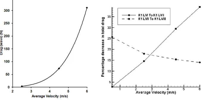
rise to steep rise of drag, which is found to be dependent upon the length of the kayak and velocity (Figure 6a).
The calculation of wave drag from CFD, due to water displacement above the waterline attributed to formation of waves around the kayak was evaluated by consideration of the volume fraction of air on the initial (unperturbed) water surface (Figure 6a). The wave drag shown is calculated for kayak K1 Vanquish model LIII. The steep rise of wave drag, due to formation of waves, at higher flow velocities is noteworthy.
For efficiency during flatwater competition, the kay-aker has to increase the paddling effort drastically, when moving at high speed, due to the sharp increase in drag. The major component of the paddler’s power output is expended in maintaining the kayak’s relatively constant velocity (power = drag force × kayak velocity). Thus, the power expected from the paddler is proportional to the kayak velocity cubed. The endeavor to accelerate the kayak moving at higher velocities will become more and more intricate, and will depend upon the efficiency of skill and physiological factors of kayaker. The disturbance added to the flow by the paddle motion has not been accounted for in the current study, which has been carried out under steady-state conditions. The fluctuation velocity is estimated by solving the turbulent model equations, and the numerical calculation procedure takes into account the summation term of mean and fluctuating velocity components.
The percentage variation in total drag due to form and friction at various flow velocities conveys that there is noticeable improvement in design from K1 Vanquish LI to LII, with a subsequent rise of percentage reduc-tion in total drag with rise in flow velocity (Figure 6b). It can be deduced that the K1 Vanquish LII model was
improved to function well at high speeds encountered in competitions. The gentle fall of percentage reduction in total drag with the rise in flow velocity for design transformation from models LII to LIII conveys further optimization of hydrodynamic geometric parameters for efficiency at higher velocities. There are few quantities that can be changed to produce a higher average velocity against drag to achieve faster paddling times for a given paddler’s power output. The total weight of the paddler is an important contributor to drag. Body weight affects not only the wave drag created but also the wetted surface area. In addition, the cross-sectional area of the kayak that is submerged in water also contributes to drag. The friction drag created as a result of the semi-submerged kayak can be minimized by a reduction in either wetted area or a reduction of the friction coefficient.14 Thus it
would appear that not only should the power-to-weight ratio of the paddler be optimized,27 but matching blade
size to event distance, paddling skill level, metabolic fitness, and the athlete’s strength are also essential com-ponents to paddling success.
The transformation in hydrodynamic effect attributed to the differences in hull geometrical shape was deduced by comparative analysis among the kayak models by considering the viscous and pressure drag and their coef-ficients. Moreover, confirmatory comparative analyses between CFD and the calculated geometrical param-eters demonstrate and reaffirm a progressive evolution in design. A simplified approach of the current study allowed the effective geometric study of the hull shapes based upon drag with an identified reduction—which could easily be the difference between Olympic glory and the ignominious defeat.
Figure 6 — (Left) The variation of drag due to formation of waves versus average velocity corresponding to the K1 Vanquish LIII kayak model and (right) the variation of percentage change in total drag for successive kayak evolution models versus average velocity with reference to the K1 Vanquish LIII model.
This study can find application during selection and training, when a coach can select the kayak with better hydrodynamics and improve overall race time by additional improvement in paddling effort by the athlete aided with the hydrodynamics of the kayak during the various phases of a kayak race. In addition, this study is very important for kayak manufacturers for further enhancement in hull design, with better hydrodynamics aiding improvement in race times.
Acknowledgments
The authors would like to acknowledge Manuel Ramos, Nuno André Santos, João Passos, and João Costa, from MAR Kayaks, Lda. for all the support during this project. The current research has been supported by the Portuguese Government and Euro-pean Union by grants of the Science and Technology Foundation (PTDC/DES/098532/2008) and QREN (Process no. 4608, SI I&DT 17/2008, Vale I&DT).
References
1. Canoe/Kayak Slalom. Beijing 2008 Olympic Games Offi-cial Website. http://en.beijing2008.cn/sports/canoekayak-slalom.Upated August 8–24, 2008. Accessed March 24, 2010.
2. Baudouin A, Hawkins D. A biomechanical review of factors affecting rowing performance. Br J Sports Med. 2002;36:396–402. PubMeddoi:10.1136/bjsm.36.6.396 3. Van Someren KA, Phillips GR, Palmer GS. Comparison of
physiological responses to open water kayaking and kayak ergometry. Int J Sports Med. 2000;21:200–204. PubMed doi:10.1055/s-2000-8877
4. Sanders RH, Kendal SJ. A description of Olympic flat-water kayak stroke technique. Aust J Sci Med Sport. 1992;24:25–30.
5. Soper C, Hume PA. Reliability of power output during rowing changes with ergometer type and race distance. Sports Biomech. 2004;3:237–248. PubMed doi:10.1080/14763140408522843
6. Liow DK, Hopkins WG. Velocity specificity of weight training for kayak sprint performance. Med Sci Sports
Exerc. 2003;35:1232–1237. PubMeddoi:10.1249/01. MSS.0000074450.97188.CF
7. McKean MR, Burkett B. The relationship between joint range of motion, muscular strength, and race time for sub-elite flat water kayakers. J Sci Med Sport. 2010;13:537– 542. PubMeddoi:10.1016/j.jsams.2009.09.003
8. Bugalski TJ. Hydromechanics For Development Of Sprint Canoes For The Olympic Games. Web blog post. https:// www.hckt.org/hcktblog/wp-content/uploads/2009/09/ HydromechanicsofSprintCanoes.pdf. Updated September 6, 2009. Accessed March 24, 2010.
9. Hanna RK. Going Faster, Higher and Longer in Sport with CFD. In: Haake S, ed. The Engineering of Sport. Rotter-dam, Netherlands: Taylor and Francis Press; 2006:3–10. 10. Robinson MG, Holt LE, Pelham TW. The technology of
sprint racing canoe and kayak hull and paddle designs.
International Sports Journal. 2002;6:68–85.
11. Soper C, Hume PA. Towards an ideal rowing technique for performance: the contributions from biomechanics. Sports
Med. 2004;34:825–848. PubMed doi:10.2165/00007256-200434120-00003
12. Peters M. Computational Fluid Dynamics for Sport
Simulation.1st ed. Eppelheim, Trondheim, Stockholm: Springer Press; 2010.
13. Ozdemir YH, Bayraktar S, Yilmaz T. Computational Inves-tigation of Hull. In: Cassella P, ed. The 2nd International
Conference on Marine Research and Transportation, Ischia, Naples, Italy. 2007:145-149. www.icmrt07.unina. it/Proceedings/Papers/A/49.pdf. Accessed March 24, 2010.
14. Jackson PS. Performance prediction for Olympic Kayak. J Sports Sci. 1995;13:239–245. PubMed doi:10.1080/02640419508732233
15. Lazauskas L, Tuck EO. Low drag racing kayaks. The Cyberiad website. http://www.cyberiad.net/library/kayaks/ racing/racing.htm. December 21, 1996. Accessed March 24, 2010.
16. Lazauskas L, Winters J. Hydrodynamic drag of some small sprint kayaks. The Cyberiad website. http://www.cyberiad. net/library/kayaks/jwsprint/jwsprint.htm. October 30, 1997. Accessed March 24, 2010.
17. Crotti F, Mazzini D, Beghini M, Barone S. Olympic Kayak Makes Waves. Elliott Kayaks website. http://www.elliott-kayaks.com.au/kayakwaves.pdf. July 29, 2005. Accessed March 24, 2010.
18. Tzabiras GD, Polyzos SP, Sfakianaki K, et al. Experimental and Numerical Study of the Flow Past the Olympic Class K-1 Flat Water Racing Kayak at Steady Speed. The Sport
Journal. http://www.thesportjournal.org/tags/volume-13-number-4.Olympic Edition.
19. Grail B. The big kayak test results. Retrieved July 18, 2011, from http://www.rapidascent.com.au/PDF/Kayak-Test_1_Intro.pdf. Updated July 30, 2006. Accessed March 24, 2010.
20. Hunter D. Speed test on various multisport kayaks and k1’s. Website. http://home.clear.net.nz/pages/racersedge/ images/Kayak speed comparison.xls. 2006. Accessed March 24, 2010.
21. Nelo K1 Vanquish III L., M.A.R. Kayaks Lda. website. http://www.mar-kayaks.pt/en/kayaks/details/k1_van-quish_iii_l. Updated 2009. Accessed March 24, 2010. 22. Rawson KJ, Tupper EC. Basic Ship Theory. 5th ed.
Woburn, MA: Butterworth-Heinemann; 2001.
23. Hinze JO. Turbulence. 1st ed. New York: McGraw-Hill Publishing Co.; 1975.
24. Wilcox DC. Turbulence Modeling for CFD. 1st ed. La Canada, California, USA: DCW Industries Press; 1998. 25. FLUENT 6.3 Documentation. High Performance
Comput-ing Environment Web site. http://hpce.iitm.ac.in/website/ Manuals/Fluent_6.3/Fluent.Inc/fluent6.3/help/index.htm. Updated September 20, 2006. Accessed March 24, 2010. 26. Patankar SV. Numerical Heat Transfer and Fluid Flow. 1st
ed. Washington, DC: Hemisphere Publishing Corporation; 1980.
27. Ackland TR, Ong KB, Kerr DA, Ridge B. Morpho-logical characteristics of Olympic sprint canoe and kayak paddlers. J Sci Med Sport. 2003;6:285–294. PubMed doi:10.1016/S1440-2440(03)80022-1