www.biogeosciences.net/10/5931/2013/ doi:10.5194/bg-10-5931-2013
© Author(s) 2013. CC Attribution 3.0 License.
Biogeosciences
Geoscientiic
Geoscientiic
Geoscientiic
Geoscientiic
Temporal and spatial variations of soil CO
2
, CH
4
and N
2
O fluxes at
three differently managed grasslands
D. Imer, L. Merbold, W. Eugster, and N. Buchmann
Grassland Sciences Group, Institute of Agricultural Sciences, ETH Zurich, Zurich, Switzerland
Correspondence to:D. Imer ([email protected])
Received: 26 January 2013 – Published in Biogeosciences Discuss.: 14 February 2013 Revised: 26 July 2013 – Accepted: 5 August 2013 – Published: 10 September 2013
Abstract.A profound understanding of temporal and spatial variabilities of soil carbon dioxide (CO2), methane (CH4)
and nitrous oxide (N2O) fluxes between terrestrial
ecosys-tems and the atmosphere is needed to reliably quantify these fluxes and to develop future mitigation strategies. For man-aged grassland ecosystems, temporal and spatial variabili-ties of these three soil greenhouse gas (GHG) fluxes occur due to changes in environmental drivers as well as fertil-izer applications, harvests and grazing. To assess how such changes affect soil GHG fluxes at Swiss grassland sites, we studied three sites along an altitudinal gradient that cor-responds to a management gradient: from 400 m a.s.l. (in-tensively managed) to 1000 m a.s.l. (moderately intensive managed) to 2000 m a.s.l. (extensively managed). The alpine grassland was included to study both effects of extensive management on CH4 and N2O fluxes and the different
cli-mate regime occurring at this altitude. Temporal and spatial variabilities of soil GHG fluxes and environmental drivers on various timescales were determined along transects of 16 static soil chambers at each site. All three grasslands were N2O sources, with mean annual soil fluxes ranging from
0.15 to 1.28 nmol m−2s−1. Contrastingly, all sites were weak CH4 sinks, with soil uptake rates ranging from −0.56 to
−0.15 nmol m−2s−1. Mean annual soil and plant respiration losses of CO2, measured with opaque chambers, ranged from
5.2 to 6.5 µmol m−2s−1. While the environmental drivers and their respective explanatory power for soil N2O
emis-sions differed considerably among the three grasslands (ad-justedr2ranging from 0.19 to 0.42), CH4and CO2soil fluxes
were much better constrained (adjustedr2ranging from 0.46 to 0.80) by soil water content and air temperature, respec-tively. Throughout the year, spatial heterogeneity was partic-ularly high for soil N2O and CH4 fluxes. We found
perma-nent hot spots for soil N2O emissions as well as locations of
permanently lower soil CH4uptake rates at the extensively
managed alpine site. Including hot spots was essential to ob-tain a representative mean soil flux for the respective ecosys-tem. At the intensively managed grassland, management ef-fects clearly dominated over efef-fects of environmental drivers on soil N2O fluxes. For CO2 and CH4, the importance of
management effects did depend on the status of the vegeta-tion (LAI).
1 Introduction
About 10 % of the fossil fuel emissions that originate from EU-25 countries have been shown to be absorbed by ter-restrial ecosystems (Janssens et al., 2003; Schulze et al., 2009). While most of the atmospheric CO2 is sequestered
by forests, grasslands are a small net sink for atmospheric CO2. Croplands are reported to be CO2 neutral, and
man-aged peatlands act as net sources for atmospheric CO2(Ciais
et al., 2010b). However, the net terrestrial sink for atmo-spheric CO2 is almost counterbalanced by CH4 and N2O
emissions from agriculture (Ciais et al., 2010a). Despite the relatively small atmospheric concentrations of CH4and N2O,
these two greenhouse gases (GHG) account for 26 % of the global warming effect due to their high global warming po-tential (GWP) on a per-mass basis over a 100 yr time hori-zon (IPCC, 2007). Thus, understanding temporal and spatial variabilities of soil CO2, CH4 and N2O fluxes between
grasslands is still highly uncertain, Soussana et al. (2007) and Schulze et al. (2009) estimated that European grasslands had negative GWPs (including vertical and lateral fluxes of the three GHGs: e.g., fertilizer input, harvested biomass, ani-mal emissions). In particular, all these investigated European grasslands were net sinks for CO2on an annual timescale.
Soil fluxes of CH4and N2O, expressed in CO2equivalents,
reduced the net CO2 sink capacity, but were too small to
change the overall effect into a positive GWP (Soussana et al., 2007; Schulze et al., 2009). These two studies, how-ever, did not consider grasslands at higher elevations, with cooler and wetter climatic conditions that may subsequently lead to higher soil CH4 and N2O emissions. Mountain
re-gions are characterized by more orographic precipitation un-der episodic influences of maritime air masses, with lower evapotranspiration rates due to lower temperatures, both con-tributing to wetter soils (Beniston, 2005) and potentially higher soil emissions of CH4and N2O.
Many studies used manually operated closed soil cham-bers to measure soil fluxes of CO2, CH4 and N2O (Flessa
et al., 2002; Pumpanen et al., 2004; Wang et al., 2005; Jones et al., 2006; Jiang et al., 2010; Rochette, 2011), as they are applicable in a wide range of ecosystems with varying site conditions. Moreover, chamber methods, in contrast to the eddy covariance method, are capable of detecting small flux magnitudes that are characteristic for CH4and N2O fluxes
between climatic- or management-driven pulse events (Bdocchi et al., 2012). In addition, the use of chambers al-lows for detection of spatial patterns in GHG fluxes (Flessa et al., 2002; Merbold et al., 2011), an important aspect when studying managed or undulating grassland sites (Am-bus and Christensen, 1994; Ball et al., 1997; Mathieu et al., 2006). Especially N2O and CH4fluxes are known for their
non-uniform spatial distribution of sources and sinks (e.g., Matthias et al., 1980; Folorunso and Rolston, 1984; van den Pol-van Dasselaar et al., 1998). The spatial patterns are often controlled by grazing, vegetation and soil properties such as soil type and texture, soil temperature and soil water content, as well as soil C and N contents and microtopography (e.g., Dalal and Allen, 2008). In managed grasslands, temporal variability of soil GHG fluxes needs to be taken into consid-eration additionally since flux magnitudes respond not only to environmental forcings but also to human-induced activi-ties such as harvesting and fertilization (Buchmann, 2011).
To understand how annual soil GHG fluxes respond to environmental- and management-induced forcings, we quan-tified temporal and spatial variations of chamber-based soil CO2, CH4and N2O fluxes at three Swiss grasslands, which
are part of a traditional three-stage farming system at differ-ent altitudes (Weiss, 1941; Boesch, 1951; Ehlers and Kreutz-mann, 2000). Our specific objectives were as follows: (1) to investigate the source/sink behavior of soil CO2, CH4 and
N2O fluxes at three differently managed grasslands located
along an altitudinal gradient under different climatic condi-tions; (2) to assess temporal variation of soil GHG fluxes at
seasonal and annual timescales; and (3) to identify the spatial variations within sites.
2 Materials and methods 2.1 Site description
The three-stage farming system that is typical for many parts of the Swiss Alps (Ehlers and Kreutzmann, 2000) was represented exemplarily by the three ETH research sites Chamau (CHA), Fr¨ub¨ul (FRU) and Alp Weissenstein (AWS). The lowland site is represented by Chamau, situated north of Lake Zug in the pre-alpine lowlands of Switzerland at 400 m a.s.l. (47◦12′37′′N, 8◦24′38′′E), with a mean annual temperature of 9.1◦C and 1151 mm of precipitation (Sieber et al., 2011; Finger et al., 2013). The dominating soil type at CHA is a Cambisol (pH=5) with bulk density ranging be-tween 0.9 and 1.2 103kg m−3 in the uppermost 20 cm. The grass mixture consists of two dominating species, i.e., Italian ryegrass (Lolium multiflorum Lam.) and white clover ( Tri-folium repensL.). In 2010 and 2011, the pastures were used for forage production (Sautier, 2007; Zeeman et al., 2010). The site is intensively managed, with 5 to 10 management events per calendar year, including harvests and subsequent slurry applications. The exact number of management events per calendar year naturally depends on seasonal weather con-ditions.
The so-called Maiensaess site (early season moun-tain rangeland) is represented by Fr¨ub¨ul, situated at the Zugerberg mountain ridge, east of Lake Zug (47◦6′57′′N, 8◦32′16′′E) at 1000 m a.s.l., with a mean annual tempera-ture of 6.1◦C and 1682 mm of precipitation (Sieber et al., 2011; Finger et al., 2013). At FRU, the dominating soil type is a Gleysol (pH=4.5), with bulk density ranging be-tween 1.3 and 1.4 103kg m−3(uppermost 20 cm). The grass mixture is more diverse than at CHA, consisting of rye-grass (Lolium multiflorum Lam.), meadow foxtail ( Alopecu-rus pratensis L.), cocksfoot grass (Dactylis glomerata L.), dandelion (Taraxacum officinale), buttercup (RanunculusL.) and white clover (Trifolium repensL.) (Sautier, 2007; Zee-man et al., 2010). The pastures at FRU are used for cattle grazing in late spring (May) and early fall (September). The management includes two to four harvests and/or fertiliza-tion events (slurry/manure) per calendar year, depending on local weather conditions and resulting vegetation growth.
CHA
400 m a.s.l. FRU 1000 m a.s.l.
AWS 2000 m a.s.l.
50 km 100 m
CHA
1 16
100 m
1
9
16 12
100 m
AWS
1
16
(a) (b)
(d) (c)
Fig. 1.Topographical map of Switzerland(a)showing the geographic position of the sites,(b)Chamau (CHA),(c)Fr¨ub¨ul (FRU) and(d)Alp Weissenstein (AWS) as well as site setup maps(b–d). The red star indicates the position of the eddy covariance tower, and the red dots the position of the chambers along the prevailing wind direction (flux footprint; modified after Zeeman et al., 2010). The numbers refer to the chamber numbers along the transects. Dots denote individual trees, and gray bold lines paved roads.
alpinae, with red fescue (Festuca rubra), alpine cat’s tail (Phleum rhaeticum), white clover (Trifolium repens L.) and dandelion (Taraxacum ofcinale) (Sautier, 2007; Zeeman et al., 2010). AWS represents the summer rangelands for cat-tle grazing without harvests in normal years. Manure is ap-plied to the pastures at the end of the grazing season, typi-cally in the second half of September. The geographic loca-tion of the three sites as well as the site setups are shown in Fig. 1, while dates for harvests and fertilization events are shown in Table 1.
2.2 Experimental setup
From June 2010 to June 2011, we measured soil fluxes of CO2, CH4 and N2O using opaque static soil chambers
at all three sites. The diameter of the polyvinyl chloride chambers was 0.3 m, the average headspace height 0.136 m (±0.015 m) and average insertion depth of the collars was 0.08 m (±0.05 m). On sampling campaigns with vegetation inside the chamber >0.20 m , collar extensions (0.45 m) were used. Chamber lids were equipped with reflective alu-minum foil to minimize heating inside the chamber during the period of actual measurement. At each site, transects of 16 soil chamber collars were installed in May 2010 (Fig. 1). Spacing between the chambers was 7 m at CHA and FRU, and 5 m at AWS. At FRU, two transects were established, one consisting of 12 chambers and a second consisting of four
chambers (Fig. 1c). This was done to adopt the sampling ap-proach to the usual management regime, which is coerced by two differently managed field parcels. Spacing was chosen so that the transects would fit into the previously calculated footprint of the eddy covariance towers at the respective sites (Zeeman et al., 2010), as well as to cover the topographic differences at each site. At FRU and AWS, chamber collars were fenced to avoid trampling and/or removal by the cattle. Sampling of the chambers was performed on a weekly basis during the growing season, and at least once a month during the winter season (except for AWS, which is inaccessible in winter). The vegetation inside the chamber collars was man-ually harvested at the times of regular management activities, i.e., harvests and grazing.
Additionally, we measured diel patterns of soil CH4 and
N2O fluxes in an intensive observation campaign in
Septem-ber 2010. During this campaign, soil CH4 and N2O fluxes
were measured over 48 consecutive hours at all three sites simultaneously, at intervals of two hours. During this 48 h intensive observation campaign (21–23 September 2010), 75 mean chamber fluxes of CH4and N2O were obtained at the
Table 1.Management activities (harvests and fertilization: SL=slurry; MA=manure) and nitrogen inputs (kg N ha−1) during flux mea-surement periods at the three sites Chamau (CHA), Fr¨ub¨ul (FR) and Alp Weissenstein (AWS). Numbers indicate nitrogen inputs from slurry/manure in kg ha−1. At AWS, no harvest was performed (–).
CHA FRU AWS
Cuts 20 Aug 2010 2 Jul 2010 –
2 Oct 2010 2 Aug 2010 21 Apr 2011
15 Jun 2011
Fertilization 6 Jul 2010 SL, 18 19 Jul 2010 MA, 33 30 Aug 2010 MA, n.a. 25 Aug 2010 SL, 30 11 Sep 2010 SL, 10
28 Oct 2010 SL, 44 23 Mar 2011 SL, 140 10 Mar 2011 SL, 60
28 Apr 2011 SL, 35 22 Jun 2011 SL, 52
2.3 Data acquisition and processing 2.3.1 Flux sampling and calculations
GHG fluxes were calculated based on the rate of changing gas concentrations inside the chamber headspace. After clos-ing the chambers, four samples were taken, one immediately after closure and then at 10 to 13 min increments so that the chamber was no longer closed than 40 min. This clos-ing time was sufficiently short to avoid saturation effects in-side the chamber headspace. We inserted 60 mL syringes into the chambers lid septums to take the gas samples, and then injected the gas into pre-evacuated 12 mL vials (Labco Lim-ited, Buckinghamshire, UK). Prior to the second, third and fourth sampling of each chamber, the chamber headspace was flushed with the syringe volume of air from the cham-ber headspace to minimize effects of built-up concentration gradients inside the chamber. Gas samples were analyzed for their CO2, CH4and N2O concentrations using gas
chro-matography (Agilent 6890 gas chromatograph equipped with a flame ionization detector, a methanizer and an electron cap-ture detector, Agilent Technologies Inc., Santa Clara, USA) as described by Hartmann et al. (2011).
Data processing, which included flux calculation and qual-ity checks, was carried out with the R statistical software (R Development Core Team, 2010). The rate of change was cal-culated by the slope of the linear regression between gas con-centration and time. Fluxes were always small enough (r2 and visual inspection of concentration changes with time) that no saturation in measured concentration data could be detected that would be indicative of saturation effects inside the chamber. We used the following equation to derive the flux estimateFGHG:
FGHG=
δc δt ·
p·V
R·T·A, (1)
wherecis the respective GHG concentration (µmol mol−1 for CO2; nmol mol−1for CH4and N2O). Time (t) is given in
seconds, atmospheric pressure (p) in Pa, the headspace vol-ume (V) in m3, the universal gas constant (R) is 8.3145 m3 Pa K−1mol−1, T is ambient air temperature (K) and Ais the surface area enclosed by the chamber (m2). Individual
chamber fluxes were only computed if the linear regression for each individual GHG yielded ar2≥0.8. If the slope be-tween the first and second concentration obviously deviated from the one of the remaining three concentration measure-ments, then we omitted it and calculated the flux from the remaining three. Chambers for which the rate of change of CO2was negative were also discarded, as photosynthesis is
assumed to be zero inside the opaque chamber. The mean chamber flux was then calculated as the arithmetic mean of all available individual chamber fluxes for each date and site. A total of 81 sampling campaigns were performed be-tween June 2010 and June 2011 (NCHA=35; NFRU=32;
NAWS=17), resulting in an equivalent number of mean
chamber fluxes of N2O, CH4 and CO2. We follow the
mi-crometeorological convention, where positive fluxes are di-rected to the atmosphere, and negative fluxes to the ecosys-tem.
2.3.2 Ancillary measurements
At each field site, the following environmental variables were recorded in the center of the transects (eddy covari-ance towers, Fig. 1) as 10 min averages: air temperature (Ta) at 2 m (HydroClip S3, Rotronic AG, Basserdorf, CH),
soil temperature (Ts) at −0.02 m (TL107 sensors,
Marka-sub AG, Olten, CH), volumetric soil water content (SWC) at
Fig. 2.Annual courses of N2O, CH4and CO2fluxes at Chamau (CHA), Fr¨ub¨ul (FRU) and Alp Weissenstein (AWS). The black lines indicate
the mean soil flux of the respective greenhouse gas (GHG), and the gray-shaded areas indicate the 95 % confidence intervals. Dashed, vertical lines indicate fertilizer applications. Black boxes for FRU and CHA denote periods of permanent snow cover. Note the different scaling for N2O fluxes at the three sites. Fluxes of N2O and CH4are given in nmol m−2s−1and CO2in µmol m−2s−1.
USA), i.e., every week during the growing period and at least monthly during winter (when there was no snow cover). LAI measurements represent averages of 12 measurements along the chamber transects.
2.3.3 Statistics
For each site, mean chamber GHG fluxes were used to estab-lish functional relationships with environmental drivers on annual timescales, using stepwise multiple linear regression models for annual timescales. A standardized principal com-ponent analysis (PCA) was performed prior to the multiple linear regressions to minimize potential artifacts from co-linearities between environmental drivers. Since CH4fluxes
at CHA and FRU showed exponential relationships with soil water content, data were log-transformed for the respec-tive multiple linear models. The relarespec-tive importance of each driver within the regression model was estimated using hier-archical partitioning (Chevan and Sutherland, 1991). The un-certainty of the calculated relative importance was assessed using parametric bootstrapping methods (Efron, 1979).
To investigate spatial variability of GHG fluxes, a one-way analysis of variance (ANOVA) was performed. The chamber number along the transect (Fig. 1) was used as a predictor, and all valid annual flux values per chamber were included. To assess the statistical significance of pairwise comparisons
of ANOVA results, the Tukey honestly significant differences (HSD) test was chosen.
3 Results
3.1 Temporal variation of GHG fluxes 3.1.1 Seasonal flux patterns and management
Soil fluxes of N2O and CO2showed a commonly known
sea-sonal pattern, with highest emission rates during the summer months (Fig. 2). Soil emissions of CH4were mostly observed
during winters, whereas uptake rates were prevailing in sum-mers.
At all three sites, soil N2O fluxes were mostly positive,
in-dicating a source for N2O. Occasional uptake was observed
for mean and individual chamber fluxes, as indicated by the 95 % confidence interval in Fig. 2. Highest N2O efflux rates
were observed at CHA (intensively managed) shortly after slurry applications. These peak fluxes exceeded maximum N2O fluxes at FRU (moderately managed) and AWS
study period was highest at CHA with 1.28 nmol m−2s−1,
and lowest at FRU with 0.15 nmol m−2s−1. At AWS, an
av-erage efflux of 0.23 nmol m−2s−1 was observed. The low
mean N2O efflux at FRU is likely due to low emission
rates during winter, which were missing from the AWS data. Hence mean emissions were larger at AWS than at FRU.
At CHA and FRU, both positive and negative methane fluxes were observed, yet uptake dominated at both sites. During eight sampling campaigns, which represented 20 % of all campaigns, CHA was a source of CH4. FRU was a
source during five sampling dates, representing 12.5 % of all campaigns, while AWS acted as a sink for atmospheric CH4throughout the measurement period. However, no
mea-surements are available for the winter period at this site, due to the inaccessibility of the site. The response of CH4
fluxes to fertilization, i.e., reduced uptake rates, was not as distinct as for N2O fluxes. Over the 12-month study
pe-riod, mean uptake rates for CH4 were −0.15, −0.22 and
−0.56 nmol m−2s−1at CHA, FRU and AWS, respectively. Temporal flux patterns of CO2 were comparable at all
three sites. The annual range of flux magnitudes was slightly smaller at AWS than at CHA and FRU. Respiration in-creased after fertilization at all three sites, yet the magni-tude of this response was variable (Fig. 2). Over the 12-month study period, mean respiration rates were 6.5 and 6.3 µmol m−2s−1 at CHA and FRU, respectively. At AWS, respiration rates were slightly smaller, with an overall mean flux of 5.2 µmol m−2s−1(growing season average).
3.1.2 Seasonal response of fluxes to environmental drivers
With the PCA, we were able to identify similarities among potential driver variables (Ta,Ts, SWC, PAR and LAI) and
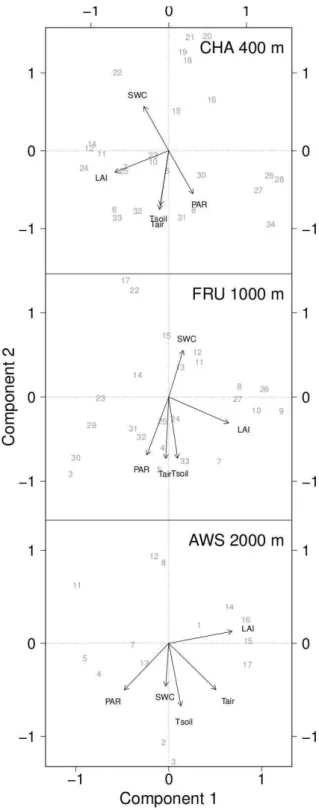
to reduce the set of driver variables for exploring functional relationships to those drivers that (a) are as independent from each other as possible, and (b) that are of similar relevance at all three elevations, such that functional relationships built with the selected drivers can be compared among sites. Ni-trogen inputs in the form of slurry/manure applications were not considered for the PCA, as only six and three data points would have been available at CHA and FRU, respectively, and LAI can already be seen as a proxy for management activity. At CHA and FRU,Ta andTs had similar loadings
(Fig. 3) because both followed a similar annual cycle. Since Ta generally had the higher explanatory power thanTs, we
selectedTa. The first and second principal components
fur-ther indicated that PAR and SWC may be treated as one vari-able at CHA and FRU (Fig. 3), where variations in PAR were of opposite sign compared to variations in SWC, simply in-dicating that episodic increases in SWC after rain events at the lower two sites coincided with periods of high cloudi-ness that reduced PAR over several days. In contrast, un-der fair weather conditions, the typical diurnal cycle of PAR was likely linked to a similar cycle of SWC in the opposite
Fig. 3. Biplots of the first two components of a standardized principal component analysis of environmental variables for the three sites Chamau (CHA), Fr¨ub¨ul (FRU) and Alp Weissenstein (AWS). Environmental variables measured during sampling cam-paigns within the 12-month study period were considered (num-bers 1 to maximum 34 at CHA). Ta=air temperature;Ts=soil
direction. Since our selection ofTa already represented
at-mospheric conditions at a site, we selected SWC instead of PAR as the second variable. The third variable selected via PCA was LAI, which was almost independent of SWC at all three sites (Fig. 3), and hence was expected to add ex-planatory value to a functional model where the three com-partments atmosphere (Ta), soil (SWC) and vegetation (LAI)
were represented (Fig. 4).
The explanatory power of the multiple linear model with regard to the temporal variation of N2O fluxes varied
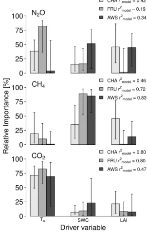
consid-erably at the three sites, with adjustedr2values ranging from 0.19 to 0.42. The relative importance (RI) of each selected driver, i.e., the contribution to the overall variance of flux variability explained by the model, was not consistent among sites (Fig. 4). At CHA, the model was able to explain 42 % of the total variance inherent in annual soil N2O flux data, with
LAI andTa being the most important explanatory variables
(RILAI=45 %; RITa=38.9 %). SWC had much less
influ-ence on the N2O efflux, with a RI of 16.1 %. At FRU,Tawas
clearly the most important driver, with a RI of 84.7 %, fol-lowed by SWC with a RI of 14 %. LAI was of minor impor-tance, with a RI of 1.3 %. In total, only 19 % of the variance in soil N2O fluxes was explained by the model at FRU. At
AWS, 34 % of the variance was explained. Here, SWC was the most powerful explanatory variable, with a RI of 54.7 %, followed by LAI (RI=43.7 %).Tahad almost no impact on
the variability of the N2O flux at AWS (RI=1.7 %) (Fig. 4).
The variation of explanatory power among the driver vari-ables within the multiple linear model for the prediction of CH4 fluxes was more pronounced than that for N2O fluxes.
However, soil CH4fluxes were better constrained by the set
of drivers, with adjustedr2values ranging from 0.46 to 0.83. Again, the RI of the drivers was not consistent among sites (Fig. 4). At CHA, the model explained 46 % of the total vari-ance inherent in all annual soil CH4flux data, with LAI and
SWC being the most influential variables (RILAI=45.4 %;
RISWC=35.4 %), followed by Ta with a RI of 19.2 %. At
FRU, 72 % of the total variance was explained, with SWC being the most important variable, exhibiting a RI of 89 %. At AWS, 83 % of variance was explained by the model, of which 82.7 % were due to changes in SWC. At both sites, FRU and AWS, the variables LAI andTa had minor
influ-ences on soil CH4fluxes.
The explanatory power of the multiple linear model for soil CO2fluxes was almost the same at CHA and FRU, with
80 % total explained variance. At AWS, the model was still able to explain 47 %. At CHA and FRU, Ta was the most
influential variable, with RI values of 71 and 81 %, respec-tively. Yet, at CHA, LAI had a considerable influence on the temporal variability of CO2fluxes, with a RI of 21.8 %. At
FRU, the contribution of seasonal changes in LAI was less important (RI=9.1 %). At AWS, Ta was the most
impor-tant variable in the model similar to CHA and FRU (RI of 55.7 %), followed by SWC with a RI of 30.9 % (Fig. 4).
0 25 50 75 100
CHA r2model = 0.42
FRU r2model = 0.19
AWS r2
model = 0.34 N2O
0 25 50 75 100
CHA r2model = 0.46
FRU r2
model = 0.72
AWS r2model = 0.83
CH4
Relativ
e Impor
tance [%]
0 25 50 75 100
Ta SWC LAI
CHA r2model = 0.80
FRU r2
model = 0.80
AWS r2model = 0.47
CO2
Driver variable
Fig. 4.Explanatory power of driver variables for GHG fluxes on the annual timescale at Chamau (CHA), Fr¨ub¨ul (FRU) and Alp Weissenstein (AWS), withTaas air temperature, SWC as soil
wa-ter content and LAI as leaf area index. Contribution (relative im-portance) to the overall variance explained is given in %. Error bars indicate 95 % confidence intervals as determined from boot-strapping (Nruns=1000).r2values represent overall model
perfor-mance. Significance levels of each driver can be found in Table 2. The upper panel shows the model performance at all three sites for N2O fluxes, the middle panel for CH4fluxes and the lower panel
for CO2fluxes.
3.1.3 Diel variation of N2O and CH4fluxes
Mean chamber efflux rates of N2O and mean chamber uptake
rates of CH4were observed during the intensive observation
campaign at all sites in September 2010 (Fig. 5). The diel N2O flux magnitudes along the elevational transect yielded a
different ranking among sites than that observed at the annual scale. During the intensive observation campaign, highest emissions of N2O were measured at AWS, with an average
flux of 0.54 nmol m−2s−1, followed by CHA with 0.21 and FRU with 0.15 nmol m−2s−1. Diel variations of soil N2O
fluxes were clearly found only at FRU, where high emission rates were observed during the day, and smaller emissions during nights (Fig. 5).Ta was a good predictor for N2O
●●●● ●●●●●●●●●●●● ●●●●●●●●● ●●●● ●●●●●●●●●●●● ●●●●●●●●● 0 1 2 3 4 N2
O [nmol m
−
2 s
−
1 ]
CHA 400 m
●● ●● ●●● ●●●●● ●● ●●●●●●●●●● ● ●● ●● ●●● ●●●●● ●● ●●●●●●●●●● ●
FRU 1000 m
● ● ●● ● ● ● ●●● ● ● ● ● ●●●● ● ● ● ● ●● ● ● ● ●● ● ● ● ●●● ● ● ● ● ●●●● ● ● ● ● ●● ●
AWS 2000 m
●●●● ● ●● ●● ● ● ● ● ●●● ● ● ●●●● ●●● ●●●● ● ●● ●● ● ● ● ● ●●● ● ● ●●●● ●●● −1.0 −0.5 0.0 0.5 1.0 CH 4 [nmol m −
2 s
−
1 ]
12 00 12 00 12
22.09.10 23.09.10 ● ●●● ● ● ● ● ●●●●● ● ● ●● ● ●● ● ● ●●● ● ● ● ● ●●●●● ● ● ●● ● ●● ●
12 00 12 00 12
22.09.10 23.09.10 ● ● ● ●●●●●● ●● ● ●●●● ●●●● ●●●●●
12 00 12 00 12
22.09.10 23.09.10
Fig. 5.Diel courses of N2O (top) and CH4(bottom) fluxes at Chamau (CHA), Fr¨ub¨ul (FRU) and Alp Weissenstein (AWS). The gray-shaded
areas indicate the 95 % confidence intervals of mean chamber fluxes (black line). Measurements started at noon (12:00) on September 21 and ended at noon (12:00) on 23 September.
54 and 59 % of the variance, respectively. In contrast, N2O
emissions did not significantly correlate withTa at the diel
scale (nor at the annual scale) at AWS (Fig. 4).
Highest mean uptake rates of CH4were measured at AWS
with−0.47 nmol m−2s−1, followed by CHA and FRU with
−0.31 and−0.16 nmol m−2s−1(Fig. 5). Although
consider-able variation in soil CH4flux rates was visible at CHA and
FRU, no obvious diel trend was identified. At AWS, CH4
uptake rates were almost constant, with only very little tem-poral variation. Hence, regression analysis to determine flux drivers was not successful. At CHA, 13 % of the variance in CH4uptake rates could be explained byTa, while no
sig-nificant relationship could be established at FRU and AWS. SWC variations, important at the annual scale, were affected only slightly during the 48 h intensive observation campaign, and were therefore omitted for developing any explanatory power at the diel scale.
3.2 Spatially invariant hot spots of GHG fluxes on the seasonal scale
Spatial variability of annually averaged soil N2O fluxes, i.e.,
the flux variation among chambers along the transect, was highest at CHA (Fig. 6), in contrast to the spatial variation seen over 48 h. The one-way ANOVA with chamber as a fac-tor yielded apvalue of 0.57 for soil N2O fluxes, indicating
that all chambers showed high variation during the 12 months of measurements. At AWS, chambers one to three showed a wider range of annual average N2O efflux rates relative
to the other chambers along the transect. Yet, due to some very high flux estimates, the ANOVA yielded ap value of
0.52, indicating no significant differences among individual chambers. This suggested that the spatial variability of soil N2O fluxes was not larger than the temporal variability of
the fluxes measured at AWS. Spatial variations of annual av-erage N2O fluxes at FRU were negligible (Fig. 6), and in a
similar magnitude as at the diel scale (not shown).
Spatially invariant annual averages of soil CH4fluxes were
found at CHA and FRU (Fig. 6). At AWS, we observed a spot of significantly (p=0.02) lower CH4uptakes rates around
chambers two and three (Fig. 6).
4 Discussion
It was not a priori expected that the three grasslands at dif-ferent elevations, and thus management intensities, were all weak net sinks for CH4 due to abundant precipitation in
mountainous areas, whereas the tight coupling between soil N2O efflux rates and fertilization confirmed earlier studies.
The alpine grassland (AWS), characterized by sufficient rain-water supply and hypothesized to be a net source of CH4,
acted as a net sink of methane, given the fact that the long winter period could not be included in our measurement regime. In addition, soil N2O as well as CH4 fluxes were
● ● ● ● ● ● ● ● ● ● ● ● ● ● ● ● ● ● ● ● ● ● ● ● ● ● ● ● ● ● ● ● ● ● ● ● ● ● ● ● ● ● 0 1 2 3 4 5 6 N2
O [nmol m
−
2 s
−
1 ]
CHA 400 m
p = 0.57
● ● ● ● ● ● ● ● ● ● ● ● ● ● ● ● ● ● ● ● ● ● ● ● ● ● ● ● ● ● ● ● ● FRU 1000 m
p = 0.40
● ● ● ● ● ● ● ● ● ● ● ● ● ● ● ● ● ● ● AWS 2000 m
p = 0.52
● ● ● ● ● ● ● ● ● ● ● ● ● ● ● ● ● ● ● ● ● ● ● ● ● ● −1 0 1 2 CH 4 [nmol m −
2 s
−
1 ]
1 4 7 10 13 16
p = 0.46
Chamber number ● ● ● ● ● ● ● ● ● ● ● ● ● ● ● ● ● ● ● ● ● ● ● ●
1 4 7 10 13 16
p = 0.25
Chamber number
●
●
1 4 7 10 13 16
p = 0.02
Chamber number
Fig. 6.Box plots depicting spatial gradients of mean annual N2O and CH4chamber fluxes (1–16 onxaxis) at Chamau (CHA), Fr¨ub¨ul (FRU)
and Alp Weissenstein (AWS). Thepvalues refer to the ANOVA results with chamber as a factor. Values below 0.05 indicate significant differences among mean chamber fluxes over the 12-month study period.
4.1 Seasonal GHG fluxes and drivers of their temporal variability
4.1.1 N2O fluxes
Our measurements give strong evidence that managed grass-lands are a constant source of N2O, as hardly any uptake was
observed (Ryden, 1981; Wagner-Riddle et al., 1997; Glatzel and Stahr, 2001; Neftel et al., 2007). The small number of negative soil N2O fluxes (uptake) observed was evenly
dis-tributed throughout the 12-month study period. As expected, the intensively managed site, CHA, was the strongest source of N2O. While total N addition (per application) at CHA
was comparable to FRU, mean annual emissions were more than 8 times higher than those at FRU, leading to much higher emission factors at CHA. FRU was characterized by the lowest mean annual N2O emissions. Emission factors
at the intensively managed grassland (CHA) were on av-erage 3.1±3.6 %, and therefore considerably higher than the IPCC (2007) default value of 1.25 % (without grazing). At FRU (moderately managed), emission factors were only 0.8±0.8 %.
Our findings also underline the challenge of predicting N2O fluxes from grasslands. N2O fluxes were weakly
con-strained by a set of three environmental variables. Their fluence on the flux varied temporally and from site to site, in-dicating the importance of additional factors (e.g., land man-agement, fertilization). Yet, our results are in agreement with
previous studies, which identified air temperature and soil water content as influential variables (e.g., Wang et al., 2005; Liebig et al., 2010; Schaufler et al., 2010). The high relative importance of LAI at CHA (intensively managed) can be ex-plained by the fact that step changes in LAI due to regular harvests during the growing season reflect subsequent slurry applications at CHA (N addition usually within five days af-ter the harvest). This finding underlines the importance of a realistic management consideration when predicting N2O
fluxes. This was corroborated in Fig. 7, which shows the re-sponse of the three GHG fluxes to their primary environmen-tal driver (at two LAI classes) on the annual scale (Table 2). For N2O we found that Ta had no significant influence on
flux magnitudes at constant LAI ranges. Thus, management (with LAI as proxy) had a larger effect on N2O fluxes than
the environment (withTaas proxy).
4.1.2 CH4fluxes
Our results showed consistently small CH4sinks at all three
sites, which is in agreement with other studies on temperate grasslands at low altitudes (Mosier et al., 1997; Liebig et al., 2010). Positive soil CH4fluxes mostly occurred during
● ● ●
● ● ●
N2O
LAI = 3.5 r = 0.07 p = 0.90
1 2 4
● ●
● ●
●
● ●
●
LAI < 1.0 r = 0.47 p = 0.20
0 5 10 15 20 25 30
Air temperature
1 2 4
●
Greenhouse gas flux
●
●
● ● ● ●
CH4
LAI = 3.5 r = 0.09 p = 0.87
−0.2 0 0.2
●
● ●
● ●
● ●
●
LAI < 1.0 r = 0.76 p = 0.02
35 37 39 41 43 45 47 49
Soil water content
−0.2 0 0.2
● ● ●
● ●
●
CO2
LAI = 3.5 r = 0.65 p = 0.17
2 6 12
● ●
●
● ● ●
● ●●
LAI < 1.0 r = 0.87 p < 0.01
0 5 10 15 20 25 30
Air temperature
2 6 12
Fig. 7.Relationships of mean chamber GHG fluxes and their primary environmental drivers at two different LAI classes for the intensively managed site Chamau (CHA). For CH4and N2O, fluxes are given in nmol m−2s−1; for CO2in µmol m−2s−1. Soil water content is given in vol. %, and air temperature in◦C. Correlation coefficients andpvalues are given.
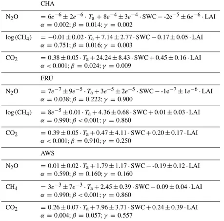
Table 2.Multiple linear model equations for annual GHG fluxes at the three sites Chamau (CHA), Fr¨ub¨ul (FRU) and Alp Weissenstein (AWS);pvalues are given for the individual drivers (Ta=air temperature; SWC=soil water content; LAI=leaf area index).
CHA
N2O =6e−6±2e−6·Ta+8e−4±3e−4·SWC−-2e−5±6e−6·LAI
α=0.002;β=0.014;γ =0.002
log(CH4) = −0.01±0.02·Ta+7.14±2.77·SWC−0.17±0.05·LAI
α=0.751;β=0.016;γ =0.003
CO2 =0.38±0.05·Ta+24.24±8.43·SWC+0.45±0.16·LAI
α <0.001;β=0.024;γ =0.009
FRU
N2O =7e−7±9e−5·Ta+3e−5±2e−5·SWC−-1e−7±1e−6·LAI
α=0.038;β=0.222;γ =0.900
log(CH4) =8e−5±0.01·Ta+4.36±0.68·SWC+0.01±0.03·LAI
α=0.990;β <0.001;γ =0.860
CO2 =0.39±0.05·Ta+0.47±4.11·SWC+0.20±0.17·LAI
α <0.001;β=0.910;γ =0.250
AWS
N2O =0.01±0.02·Ta+1.79±1.17·SWC−-0.19±0.12·LAI
α=0.590;β=0.160;γ =0.160
CH4 =3e−3±7e−3·Ta+2.45±0.39·SWC−0.09±0.04·LAI
α=0.990;β <0.001;γ =0.860
CO2 =0.26±0.07·Ta+7.96±3.71·SWC+0.24±0.39·LAI
CH4 at FRU in the years 2007, 2008 and 2009. However,
their measurements were taken in generally drier soils, sup-porting the idea of regulating effects of SWC on CH4fluxes
(RI of 89 %). At the extensively managed AWS site, both Hartmann et al. (2011) and this study exclusively observed uptake of CH4.
Annually, soil CH4fluxes were well predictable by SWC
(Liebig et al., 2010; Schrier-Uijl et al., 2010; Hartmann et al., 2011). Furthermore, at the intensively managed site (CHA), LAI had comparable explanatory power to SWC. As men-tioned before, step changes in LAI during the growing period reflect management activities (fertilization at low LAI). Al-though ammonium-based fertilizers (e.g., organic fertilizers) can inhibit CH4uptake (oxidation) by methanotrophs
(Willi-son et al., 1995; Stiehl-Braun et al., 2011), SWC still had a highly significant impact on CH4fluxes at LAI<1 (Fig. 7),
indicating dominant environmental drivers.
4.1.3 CO2fluxes
Opaque soil chambers were used to exclusively measure res-piratory fluxes of CO2, which were in the expected range
from close to zero in winter up to 15 µmol m−2s−1 during summer, similar to, e.g., Myklebust et al. (2008). At FRU, chamber measurements agreed well with eddy covariance-based respiration data, simultaneously recorded at all three sites (Fig. 8). At CHA, eddy-covariance-based fluxes were systematically higher, which is likely due to the different scale of both measurement techniques (Wang et al., 2009). Except for one outlier of eddy-covariance-based soil respira-tion, chamber measurements agreed well with eddy covari-ance data at AWS. This outlier on August 25 may be an ar-tifact of the gap-filling procedure for eddy covariance respi-ration data. Besides the the expected importance ofTa and
SWC for CO2efflux rates, LAI was once more a reasonable
predictor (RI of 21.8 %) at the intensively managed grassland (CHA). Keeping LAI constant at<1 (Fig. 7) revealed a still highly significant effect ofTaon soil CO2fluxes, supporting
the notion that management impacts on soil flux magnitudes of CO2are rather small compared to environmental drivers
(Peng et al., 2011).
4.2 Diel variation of N2O and CH4fluxes
In contrast to what we learned on the annual scale, highest emissions of N2O of all three grasslands were observed at
AWS, being twice the observed seasonal mean. As manure was applied to AWS pastures 10 days prior to sampling, we likely captured a “hot” moment, supporting our conclusion that management impacts are dominating soil N2O flux
vari-ability. Already studies by Christensen (1983) and Flechard et al. (2007) have shown that peak emissions of N2O
ap-peared lagged to manure application (8 to 12 days).
In the literature, there is no consistent picture regarding the presence of significant diel patterns of N2O and CH4
Soil and plant respir
ation b
y eddy co
var
iance [µmol m
−
2 s
− 1 ] ● ● ● ● ● ● ● ● ● ● ● ● ● ● ● ● ● ● ● ● ● ● ● ● ● ● ● ● ● ● ● ● ● ● 0 5 10 15 20 25 1:1
r2 = 0.33; y = 1.4±0.3 x + 2.8±2.4
CHA
● ● ● ● ● ● ● ● ● ● ● ● ● ● ● ● ● ● ●●●● ● ● ● ● ● ● ● ● ● ● 0 5 10 15 20 25 1:1r2 = 0.80; y = 1.1±0.1 x + 0.8±0.7
FRU
● ● ● ● ● ● ● ● ● ● ● ● ● ●0 5 10 15 20 25
0 5 10 15 20 25 1:1
r2 = 0.49; y = 1.9±0.5 x − 3.6±2.9
AWS
Soil and plant respiration by chamber [µmol m−2 s−1]
Fig. 8.Soil and plant CO2respiration rates calculated from eddy
covariance and corresponding chamber-derived values. Mean cham-ber fluxes are shown for all sampling campaigns at Chamau (CHA), Fr¨ub¨ul (FRU) and Alp Weissenstein (AWS);pvalues of the linear regressions were<0.001 at CHA and FRU, and 0.003 at AWS. Un-certainties in the model equations are standard errors.
fluxes (Christensen, 1983; Skiba et al., 1996; Maljanen et al., 2002; Duan et al., 2005; Hendriks et al., 2008; Baldocchi et al., 2012). Duan et al. (2005) suggested that the type of ecosystem might have an influence on the presence of diel soil N2O and CH4flux variations. However, our study
exclu-sively investigated grasslands, and we found significant diel variations of N2O fluxes for one out of three sites (FRU). At
CHA, changes in air temperature affected soil N2O fluxes
less strongly, and thus no significant diel patterns in N2O
that the last slurry application at CHA was more than four weeks prior to the intensive campaign (25.08.2010; slurry 30 kg N ha−1), and that the vegetation composition at FRU
exhibits a larger fraction of legumes. This suggests that not only ecosystem type, but also site specifics (e.g., manage-ment intensity or vegetation composition) might influence diel variations in soil N2O fluxes.
In contrast to what we observed on the annual scale (Ta-ble 2), CH4fluxes were not constrained by changes in SWC
over the course of 48 h, probably because changes were too small (decrease of less than 2 % vol) to significantly affect the magnitude of CH4fluxes.
4.3 Spatial patterns and autocorrelation
Working with soil chambers requires information on the spa-tial distribution of GHG fluxes at ecosystem scale to design appropriate experiments and to be able to correct mean soil fluxes for potential biases. In relation to the magnitude of mean chamber fluxes of N2O and CH4, individual chamber
fluxes are highly variable in space (e.g., Matthias et al., 1980; Folorunso and Rolston, 1984; Mosier et al., 1991), as they are largely determined by small-scale biochemical processes (Ambus and Christensen, 1994; Dalal and Allen, 2008).
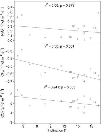
We observed that out of our three sites, only AWS ex-hibited permanent spots where CH4uptake was significantly
smaller than at the rest of the transect. This corresponded well with local microtopographical conditions, i.e., the in-clination of the terrain (Fig. 9). Chambers placed in terrain with greater inclination systematically exhibited lower SWC values (data not shown). This in turn corresponded well with what was observed at the annual scale, where lower CH4
up-take rates correlated significantly with higher SWC. At CHA and FRU, we observed that flux magnitudes varied spatially; spots of reduced CH4uptake were, however, not permanent.
Thus, the situation at CHA and FRU represents the ideal case when trying to sample a representative mean of an ecosys-tem. Omitting permanent hot spots may lead to a systematic bias in GHG flux budgets. In our case, omitting chambers one to four at AWS would have lead to an underestimation of annual CH4uptake of roughly 5 % and an overestimation of
annual N2O emissions of 56 % (both regarding annual
bud-gets). Thus, all aspects of exposition and slope should be covered when assessing flux estimates of CH4 and N2O in
sloping terrain.
5 Conclusions
Highest mean annual emissions of N2O were observed at
the intensively managed site, whereas highest uptake rates of CH4were measured at the extensively managed site. This
clearly illustrates the impact that management intensity has on the magnitude of soil N2O and CH4fluxes in grasslands.
This clearly illustrates that management acts as a major
co-1 2 3
4
5
6
7 10 8 9
11 12
13
14 15
16 r2 = 0.06; p = 0.373
N2
O [nmol m
−
2 s
−
1]
0.0 0.1 0.2 0.3 0.4 0.5 0.6 0.7
1 2
3
4
5
6 7
8 9 10
11 12
13 14 15
16 r2 = 0.56; p = 0.001
CH
4
[nmol m
−
2 s
−
1]
−0.7 −0.6 −0.5 −0.4 −0.3
1 2
3
4
5
6 7
8 9
10 11
12
13 14
15
16 r2 = 0.241; p = 0.053
Inclination [°]
CO
2
[µmol m
−
2 s
−
1 ]
3 4 5 6
3 6 9 12 15 18
Fig. 9.Annually averaged chamber fluxes of N2O, CH4and CO2
at Alp Weissenstein (AWS) plotted against inclination at the respec-tive chambers. The numbers indicate the chamber position along the transect. Regression coefficients as well aspvalues are given.
driver of CH4and N2O fluxes in grasslands in addition to the
commonly shown influences of environmental variables. We identified the known set of drivers for fluxes of CO2,
CH4and N2O fluxes (Taand SWC for N2O and CH4,
respec-tively). At the intensively managed site (CHA), LAI proved to be a good proxy for management influence on fluxes of all three GHGs.
Spatial variability, especially of soil CH4and N2O fluxes
was as high as expected. Permanent spots with lower CH4
uptake coincided with smaller inclination of the terrain on which chambers were placed. Thus, on sloping terrain, mean chamber fluxes of CH4should be estimated from an
ensem-ble that is (a) sufficient in size, (b) represents the common species composition including hot spots occurring due to grazing and (c) representative for the terrain of the site. This is important since SWC is one of the major environmental drivers of CH4exchange. For soil fluxes of N2O, we suggest
Acknowledgements. We acknowledge the help of all Grassland Sciences Group Members from ETH Zurich who participated in the intensive observation campaign. We also thank our technicians Peter Pluess and Thomas Baur for station maintenance and technical support. This study was partially funded by the European Union Seventh Framework Programme (FP7/2007–2013) under grant agreement no. 244122 (GHG-Europe). This study was further supported by COST Action ES0804 – Advancing the integrated monitoring of trace gas exchange Between Biosphere and Atmosphere (ABBA).
Edited by: K. Pilegaard
References
Ambus, P. and Christensen, S.: Measurement of N2O emission from
a fertilized grassland: An analysis of spatial variability, J. Geo-phys. Res., 99, 16549–16555, 1994.
Baldocchi, D., Detto, M., Sonnentag, O., Verfaillie, J., Teh, Y., Sil-ver, W., and Kelly, N.: The challenges of measuring methane fluxes and concentrations over a peatland pasture, Agr. Forest Meteorol., 153, 177–187, doi:10.1016/j.agrformet.2011.04.013, 2012.
Ball, B., Horgan, G., Clayton, H., and Parker, J.: Spatial variabil-ity of nitrous oxide fluxes and controlling soil and topographic properties, J. Environ. Qual., 26, 1399–1409, 1997.
Beniston, M.: Mountain climates and climatic change: An overview of processes focusing on the European Alps, Pure. Appl. Geo-phys., 162, 1587–1606, doi:10.1007/s00024-005-2684-9, 2005. Boesch, H.: Nomadismus, Transhumanz und Alpwirtschaft, Die
Alpen, 27, 202–207, 1951.
Buchmann, N.: Greenhouse gas emissions from European grass-lands and mitigation options, in: Grassland productivity and ecosystem services, edited by: LeMaire, G., Hodgson, J., and Chabbi, A., Grassland productivity and ecosystem services, CAB International, UK, 92–100, 2011.
Chevan, A. and Sutherland, M.: Hierarchical partitioning, Amer. Statistician., 45, 90–96, 1991.
Christensen, S.: Nitrious oxide emission from a soil under perma-nent grass: Seasonal and diurnal fluctuations as influenced by manuring and fertilization, Soil Biol. Biochem., 15, 531–536, 1983.
Ciais, P., Soussana, J., Vuichard, N., Luyssaert, S., Don, A., Janssens, I., Piao, S., Dechow, R., Lathi`ere, J., Maignan, F., Wat-tenbach, M., Smith, P., Ammann, C., Freibauer, A., Schulze, E., and CARBOEUROPE Synthesis Team: The greenhouse gas bal-ance of European grasslands, Biogeosciences Discuss., 7, 5997– 6050, doi:10.5194/bgd-7-5997-2010, 2010a.
Ciais, P., Wattenbach, M., Vuichard, N., Smith, P., Piao, L., Don, A., Luyssaert, S., Janssens, I., Bondeau, A., Dechow, R., Leip, A., Smith, P., Beer, C., van der Werf, G., Gervois, S., van Oost, K., Tomelleri, E., Freibauer, A., and Schulze, E.: The European carbon balance, Part 2: Croplands, Glob. Change Biol., 16, 1409– 1428, 2010b.
Dalal, R. and Allen, D.: Greenhouse gas fluxes from natural ecosys-tems, Aust. J. Bot., 56, 369–407, 2008.
Dietrich, C. and Osborne, M.: Estimation of covariance parameters in kriging via restricted maximum likelihood, Math. Geol., 23, 119–135, 1991.
Duan, X., Wang, X., Mu, Y., and Ouyang, Z.: Seasonal and diurnal variations in methane emissions from Wuliangsu Lake in arid regions of China, Atmos. Environ., 39, 4479–4487, 2005. Efron, B.: Bootstrap methods: Another look at the jackknife, Ann.
Stat., 7, 1–26, 1979.
Ehlers, E. and Kreutzmann, H.: High mountain pastoralism in Northern Pakistan, Franz Steiner Verlag, Stuttgart, 2000. Finger, R., Gilgen, A., Prechsl, U., and Buchmann, N.: An
eco-nomic assessment of drought effects on three grassland systems in Switzerland, Reg. Environ. Change, 13, 365–374, 2013. Flechard, C., Ambus, P., Skiba, U., Rees, R., Hensen, A., van
Am-stel, A., van den Pol-van Dasselaar, A., Soussana, J., Jones, M., Clifton-Brown, J., Raschi, A., Horvath, L., Neftel, A., Jocher, M., Ammann, C., Leifeld, J., Fuhrer, J., Calanca, P., Thalman, E., Pilegaard, K., Marco, C. D., Campbell, C., Nemitz, E., Harg-reaves, K., Levy, P., Ball, B., Jones, S., van de Bulk, W., Groot, T., Blom, M., Domingues, R., Kasper, G., Allard, V., Ceschia, E., Cellier, P., Laville, P., Henault, C., Bizouard, F., Abdalla, M., Williams, M., Baronti, S., Berretti, F., and Grosz, B.: Effects of climate and management intensity on nitrous oxide emissions in grassland systems across Europe, Agr. Ecosyst. Environ., 121, 135–152, 2007.
Flessa, H., Ruser, R., Schilling, R., Loftfield, N., Munch, J., Kaiser, E., and Beese, F.: N2O and CH4fluxes in potato fields:
Auto-mated measurement, management effects and temporal variation, Geoderma, 105, 307–325, 2002.
Folorunso, O. and Rolston, D.: Spatial variability of field-measured denitrification gas fluxes, Soil Sci. Soc. Am. J., 48, 1214–1219, 1984.
Glatzel, S. and Stahr, K.: Methane and nitrous oxide exchange in differently fertilised grassland in southern Germany, Plant Soil, 231, 21–35, 2001.
Hartmann, A., Buchmann, N., and Niklaus, P.: A study of soil methane sink regulation in two grasslands exposed to drought and N fertilization, Plant Soil, 342, 265–275, 2011.
Hendriks, D., Dolman, A., Van der Molen, J., and van Huissteden, J.: A compact and stable eddy covariance set-up for methane measurements using off-axis integrated cavity output spec-troscopy, Atmos. Chem. Phys., 8, 431–443, doi:10.5194/acp-8-431-2008, 2008.
IPCC, W.: The physical science basis. Contribution of working group I to the fourth assessment report of the Intergovernmental Panel on Climate Change, in: Climate Change 2007, edited by: Solomon, S., Qin, D., Manning, M., Chen, Z., Marquis, M., Av-eryt, K., Tignor, M., and Miller, H., Cambridge University Press, Cambridge, 210–215, 2007.
Janssens, I., Freibauer, A., Ciais, P., Smith, P., Nabuurs, G., Fol-berth, G., Schlamadinger, B., Huties, R., Ceulemans, R., Schulze, E., Valentini, R., and Dolman, A.: Europe’s terrestrial biosphere absorbs 7 to 12 % of European anthropogenic CO2 emissions,
Science, 300, 1538–1542, 2003.
Jiang, C., Yu, G., Fang, H., Cao, G., and Li, Y.: Short-term effect of increasing nitrogen deposition on CO2, CH4and N2O fluxes
in an alpine meadow on the Qinghai-Tibetan Plateau, China, At-mos. Environ., 44, 2920–2926, 2010.
Lessard, R., Rochette, P., Gregorich, E., Desjardins, R., and Pattey, E.: CH4fluxes from a soil amended with dairy cattle manure and
ammonium nitrate, Can. J. Soil Sci., 77, 179–186, 1997. Liebig, M., Gross, J., Kronberg, S., Phillips, R., and Hanson, J.:
Grazing management contributions to net global warming po-tential: A long-term evaluation in the northern Great Plains, J. Environ. Qual., 39, 799–809, 2010.
Maljanen, M., Martikainen, P., Aaltonen, H., and Silvola, J.: Short-term variation in fluxes of carbon dioxide, nitrous oxide and methane in cultivated and forested organic boreal soils, Soil Biol. Biochem., 34, 577–584, 2002.
Mathieu, O., Leveque, J., Heault, C., Milloux, M., Bizouard, F., and Andreux, F.: Emissions and spatial variability of N2O, N2and
nitrous oxide mole fraction at the field scale, Soil Biol. Biochem., 38, 941–951, 2006.
Matthias, A., Blackmer, A., and Bremner, J.: A simple chamber technique for field measurement of emissions of nitrous oxide from soils, J. Environ. Qual., 9, 251–256, 1980.
Merbold, L., Ziegler, W., Mukelabai, M., and Kutsch, W.: Spatial and temporal variation of CO2efflux along a disturbance
gradi-ent in a miombo woodland in Western Zambia, Biogeosciences, 8, 147–164, doi:10.5194/bg-8-147-2011, 2011.
Michna, P., Eugster, W., Hiller, R., Zeeman, M., and Wanner, H.: Topoclimatological case-study of Alpine pastures near the Al-bula pass in the Eastern Swiss Alps, Geograph. Helv., in press, 2013.
Mosier, A., Schimel, D., Valentine, D., Bronson, K., and Parton, W.: Methane and nitrous oxide fluxes in native, fertilized and cultivated grasslands, Nature, 350, 330–332, 1991.
Mosier, A., Delgado, J., Cochran, V., Valentine, D., and Parton, W.: Impact of agriculture on soil consumption of atmospheric CH4
and a comparison of CH4 and N2O flux in subartic,
temper-ate and tropical grasslands, Nutr. Cycl. Agroecosys., 49, 71–83, 1997.
Myklebust, M., Hipps, L., and Ryel, R.: Comparison of eddy co-variance, chamber, and gradient methods of measuring soil CO2
efflux in an annual semi-arid grass,Bromus tectorum, Agr. Forest Meteorol., 148, 1894–1907, 2008.
Neftel, A., Flechard, C., Ammann, C., Conen, F., Emmenegger, L., and Zeyer, K.: Experimental assessment of N2O background
fluxes in grassland systems, Tellus B, 59, 470–482, 2007. Peng, Q., Dong, Y., Qi, Y., Xiao, S., He, Y., and Ma, T.: Effects of
nitrogen fertilization on soil respiration in temperate grassland in Inner Mongolia, China, Environ Earth Sci., 62, 1163–1171, 2011.
Pumpanen, J., Kolari, P., Ilvesniemi, H., Minkkinen, K., Vesala, T., Niinist¨o, S., Lohila, A., Larmola, T., Morero, M., Pihlatie, M., Janssens, I., Yuste, J., Gruenzweig, J., Reth, S., Subke, J., Savage, K., Kutsch, W., Ostreng, G., Ziegler, W., Anthoni, P., and Hari, P.: Comparison of different chamber techniques for measuring soil CO2efflux, Agr. Forest Meteorol., 123, 159–176, 2004. R Development Core Team: R: A Language and Environment for
Statistical Computing, R Foundation for Statistical Computing, Vienna, Austria, http://www.R-project.org, ISBN 3-900051-07-0, 2010.
Rochette, R.: Towards a standard non-steady-state chamber methodology for measuring soil N2O emissions, Anim. Feed Sci.
Tech., 166–167, 141–146, 2011.
Ryden, J.: N2O exchange between a grassland soil and the atmo-sphere, Nature, 292, 235–237, 1981.
Sautier, S.: Zusammensetzung und Produktivi¨at der Vegetation im Gebiet der ETHZ-Forschungsstation Fr¨ub¨ul (ZG), MSc Thesis, Institute of Geography, University of Zurich, 2007.
Schaufler, G., Kitzler, B., Schindlbacher, A., Skiba, U., Sutton, M., and Zechmeister-Boltenstern, S.: Greenhouse gas emissions from European soils under different land use: effects of soil mois-ture and temperamois-ture, Eur. J. Soil Sci., 61, 683–696, 2010. Schrier-Uijl, A., Kroon, P., Hensen, A., Leffelaar, P., Berendse,
F., and Veenendaal, E.: Comparison of chamber and eddy covariance-based CO2and CH4emission estimates in a
hetero-geneous grass ecosystem on peat, Agr. Forest Meteorol., 150, 825–831, 2010.
Schulze, E., Luyssaert, S., Ciais, P., Freibauer, A., Janssens, I., Soussana, J., Smith, P., Grace, J., Levin, I., Thiruchittampalam, B., Heimann, M., Dolman, A., Valentini, R., Bousquet, P., Peylin, P., Peters, W., Rodenbeck, C., Etiope, G., Vuichard, N., Watten-bach, M., Nabuurs, G., Poussi, Z., Nieschulze, J., and Gash, J.: Importance of methane and nitrous oxide for Europe’s terrestrial greenhouse-gas balance, Nat. Geosci., 2, 842–850, 2009. Sieber, R., Hollenstein, L., Odden, B., and Hurni, L.: From classic
atlas design to collaborative platforms – The SwissAtlasPlatform Project, in: Proceedings of the 25th international conference of the ICA, Paris, France, 2011.
Skiba, U., Hargreaves, K., Beverland, I., O’Neil, D., Fowler, D., and Moncrieff, J.: Measurement of field scale N2O emission fluxes
from a wheat crop using micrometeorological techniques, Plant Soil, 181, 139–144, 1996.
Soussana, J., Allard, V., Pilegaard, K., Ambus, P., Ammann, C., Campbell, C., Ceschia, E., Clifton-Brown, J., Czobel, S., Domingues, R., Flechard, C., Fuhrer, J., Hansen, A., Horvath, L., Jones, M., Kasper, G., Martin, C., Nagy, Z., Neftel, A., Raschi, A., Baronti, S., Rees, R., Skiba, U., Stefani, P., Manca, G., Sut-ton, M., Tuba, Z., and Valentini, R.: Full accounting of the green-house gas (CO2, N2O, CH4budget of nine European grassland
sites, Agr. Ecosyst. Environ., 121, 121–134, 2007.
Stiehl-Braun, P., Hartmann, A., Kandeler, E., Buchmann, N., and Niklaus, P.: Interactive effects of drought and N fertilization on the spatial distribution of methane assimilation in grassland soils, Glob. Change Biol., 17, 2629–2639, 2011.
Stone, M.: Cross-validatory choice and assessment of statistical pre-dictions, J. R. Stat. Soc., 36, 111–147, 1974.
van den Pol-van Dasselaar, A., Corre, W., Prieme, A., Klemedts-son, A., Weslien, P., Stein, A., KlemedtsKlemedts-son, L., and Oenema, O.: Spatial variability of methane, nitrous oxide, and carbon diox-ide emissions from drained grasslands, Soil Sci. Soc. Am. J., 62, 810–817, 1998.
Velthof, G., van Groeningen, J., Gebauer, G., Pietrzak, S., Jarvis, S., Pinto, M., Corre, W., and Oenema, O.: Temporal stability of spatial patterns of nitrous oxide fluxes from sloping grassland, J. Environ. Qual., 29, 1297–1407, 2000.
Vleeshouwers, L. and Verhagen, A.: Carbon emission and seques-tration by agricultural land use: a model study for Europe, Glob. Change Biol., 8, 519–530, 2002.
Wang, M., Guan, D., Han, S., and Wu, J.: Comparison of eddy co-variance and chamber-based methods for measuring CO2flux in
a temperate mixed forest, Tree Physiol., 30, 149–163, 2009. Wang, Y., Xue, M., Zheng, X., Ji, B., Du, R., and Wang, Y.: Effects
of environmental factors on N2O emission from and CH4uptake
by the typical grasslands in the Inner Mongolia, Chemosphere, 58, 205–215, 2005.
Weiss, R.: Das Alpwesen Graub¨undens: Wirtschaft, Sachkultur, Recht, ¨Alplerarbeit und ¨Alplerleben, Eugen Rentsch Verlag, Erlenbach–Z¨urich, 1941.
Willison, T., Webster, C., Goulding, K., and Powlson, D.: Methane oxidation in temperate soils – effects of land-use and the chem-ical form of the nitrogen fertilizer, Chemsophere, 30, 539–546, 1995.
Zeeman, M., Hiller, R., Gilgen, A., Michna, P., Pluess, P., Buch-mann, N., and Eugster, W.: Management and climate impacts on the net CO2 fluxes and carbon budgets of three grasslands